Two-Sample Testing in High-Dimensional Models
Abstract
We propose novel methodology for testing equality of model parameters between two high-dimensional populations. The technique is very general and applicable to a wide range of models. The method is based on sample splitting: the data is split into two parts; on the first part we reduce the dimensionality of the model to a manageable size; on the second part we perform significance testing (p-value calculation) based on a restricted likelihood ratio statistic. Assuming that both populations arise from the same distribution, we show that the restricted likelihood ratio statistic is asymptotically distributed as a weighted sum of chi-squares with weights which can be efficiently estimated from the data. In high-dimensional problems, a single data split can result in a “p-value lottery”. To ameliorate this effect, we iterate the splitting process and aggregate the resulting p-values. This multi-split approach provides improved p-values. We illustrate the use of our general approach in two-sample comparisons of high-dimensional regression models (“differential regression”) and graphical models (“differential network”). In both cases we show results on simulated data as well as real data from recent, high-throughput cancer studies.
Keywords High-dimensional two-sample testing; Data splitting; -regularization; Non-nested hypotheses; High-dimensional regression; Gaussian graphical models; Differential regression; Differential network
1 Introduction and Motivation
We consider the general two-sample testing problem where the goal is to test whether or not two independent populations and , parameterized by and respectively, with , arise from the same distribution. The hypothesis testing problem of interest is
| (1.1) |
In this paper the focus is on the high-dimensional setting where the number of available samples per population ( and ) is small compared to the dimensionality of the parameter space .
In a setup where and are much larger than the ordinary likelihood-ratio test offers a very general solution to problem (1.1). It is well-known that under the likelihood ratio statistic is asymptotically distributed which then allows computation of confidence intervals and p-values. However, in settings where is large compared to sample sizes, the likelihood-ratio statistic is ill-behaved and the classical asymptotic set-up cannot be relied upon to test statistical significance.
Our approach for solving the general high-dimensional two-sample problem (1.1) is motivated by the screen and clean procedure (Wasserman and Roeder, 2009) originally developed for improved variable selection in the high-dimensional regression model. The idea is to split the data from both populations into two parts; perform dimensionality reduction on one part and pursue significance testing on the other part of the data. In more detail, on the first split we select three subsets of by screening for the most relevant parameters of population and individually but also by selecting the important parameters of the pooled data from both populations. In this way we obtain an individual model with different parameter spaces for and and a joint model which describes both populations by a common parameter space. On the second split of the data, we then can compute the likelihood ratio statistic between these two models, the so-called restricted likelihood ratio statistic. A crucial observation is that the two models are non-nested and therefore non-standard tools are needed to obtain the asymptotic null distribution. We apply the theory on model selection and non-nested hypotheses developed by Vuong (1989) to the two-sample scenario and show that the null distribution asymptotically approaches a weighted sum of independent chi-squared random variables with weights which can be efficiently estimated from the second split of the data. Importantly, the weighted sum of chi-squared approximation is invoked only in the second split, where the model dimensionalty has been reduced.
As indicated above our approach involves a screening or model selection step prior to significance testing. Our method requires that the parameter set selected by a specific screening procedure contains the true model parameter (screening property) and that the selected set is small compared to the sample size (sparsity property). The first property is needed for deriving the asymptotic null distribution, whereas the latter property justifies asymptotic approximation. The two conditions which we impose here are much weaker than requiring consistency in variable selection. We propose to use -penalized maximum likelihood estimation (Tibshirani, 1996; Fan and Li, 2001) with regularization parameter chosen by cross-validation. This sets automatically non-relevant parameter components to zero and allows for efficient screening even in scenarios with very large . penalization leads to sparse estimates and there is theoretical evidence that the screening property holds under mild additional assumptions.
In current applied statistics, a wide range of applications are faced with high-dimensional data. Parameter estimation in the “large , small ” setting has been extensively studied in theory (Bühlmann and van de Geer, 2011) and also applied with success in many areas. Since interpretation of parameters is crucial in applied science there is a clear need to assess uncertainty and statistical significance in such settings. However, significance testing in high-dimensional settings has only recently attracted attention. Meinshausen et al. (2009) and Bühlmann (2012) consider testing in the high-dimensional linear model. In the context of high-dimensional two-sample comparison Bai and Saranadasa (1996), Chen and Qin (2010), Lopes et al. (2012) and others treat testing for differences in the population means. And recently, Cai et al. (2011) and Li and Chen (2012) developed a two-sample test for covariance matrices of two high-dimensional populations.
The approach proposed in this paper tackles the high-dimensional two-sample testing in a very general setting. In our methodology and can parameterize any model of interest. In the empirical examples we show below we focus on two specific applications of our approach: (i) High-dimensional regression, where two populations may differ with respect to regression models and (ii) Graphical modelling, where the two populations may differ with respect to conditional independence structure. In analogy to the term “differential expression” as widely-used for testing means in gene expression studies, we call these “differential regression” and “differential network” respectively. Both high-dimensional regression and graphical models are now widely used in biological applications, and very often scientific interest focuses on potential differences between populations (such as disease types, cell types, environmental conditions etc.). However, to date in the high-dimensional setting, two sample testing concerning such models has not been well studied. The methodology we propose offers a way to directly test hypotheses concerning differences in molecular influences or biological network structure using high-throughput data.
The organization of the paper is as follows: Section 2 introduces the setup and the methodology: Section 2.1 explains variable screening using -regularization; Section 2.2 introduces the restricted likelihood-ratio statistic; Sections 2.3 and 2.4 derives its asymptotic null distribution and Section 2.5 shows how to compute p-values using the single- and multi-split algorithms. In Section 3 we present and give details on the two specific examples of our approach that we outlined above (differential regression and differential network). Finally, in Section 4, we evaluate our methodology on simulated and real data from two recent high-throughput studies in cancer biology.
2 Data Splitting, Screening and Non-Nested Hypothesis
Consider a conditional model class given by densities
| (2.2) |
Note that can be empty (i.e., ). Let population and , where , are both generated from the same distribution and conditional on the ’s, and are generated from and respectively.
The goal is to solve the general two-sample testing problem (1.1) given data-matrices and , representing i.i.d. random samples of and . We consider the high-dimensional case with and assume that the data generating parameters and are sparse, meaning that many of their components are equal to zero. If , we have a classical (univariate) two-sample set-up. If and is the univariate Normal distribution with mean and noise variance , , then and follow linear regression models. If and is the multivariate Normal distribution with representing the inverse covariance matrix, then and follow a Gaussian graphical model and (1.1) asks whether or not two graphical models (in short: networks) are significantly different. We will treat these two examples in detail in Section 3 and 4. We refer to the regression case as differential regression and to the graphical model case as differential network.
Our methodology for solving (1.1) is based on sample splitting and has its inspiration from the work by Wasserman and Roeder (2009). We randomly divide data from population into two parts and of equal size and proceed in the same way with population which yields and . In a first step the dimensionality of the parameter space is reduced by filtering out (potentially many) redundant components. We do this by applying a screening procedure on and separately, but also on pooled data . In this way we obtain models with lower dimensionality than the full dimension . The first model describes populations and individually using different reduced-parameter spaces, whereas the second model explains both populations jointly with a single reduced-parameter space. In a second step, we then evaluate the restricted likelihood-ratio statistic on the held-out data and and perform significance testing.
2.1 Screening and -regularization
Consider i.i.d. data with distributed according to and . We have and is supposed to be sparse.
A screening procedure selects, based on data , a set of active parameter components by a map . The map then defines the active parameter space by
There are two basic requirements on the screening procedure . Firstly, the procedure should get rid of many non-relevant components in the sense that the set of active parameter components should be small compared to . Secondly, the active parameter space should contain the true parameter . We refer to these requirements as the sparsity and screening property:
- •
Sparsity property: is small compared to .
- •
Screening property: .
Formulating the sparsity property precisely, i.e. specifying the rate at which the size of the active set can grow with , is a research topic in its own right (see also the discussion in Section 5). We do not address this topic here. The screening property guarantees that the model , selected by , is correctly specified in the sense that it contains the true density function . L1-penalized likelihood methods (Fan and Li, 2001) serve as our prime example of screening procedures. Consider estimators of the form
| (2.3) |
where denotes the conditional log-likelihood and is a non-negative regularization parameter. In the context of linear regression (2.3) coincides with the Lasso estimator introduced by Tibshirani (1996). Other important example of the form (2.3) include the elastic net (Zou and Hastie, 2005), the grouped Lasso (Yuan and Lin, 2006), the graphical Lasso (Friedman et al., 2008) or the Lasso for generalized linear models (Park and Hastie, 2007). Estimators of the form (2.3) have been shown to be extremely powerful: they are suitable for high-dimensional data and lead to sparse solutions. A screening procedure can be defined by setting
| (2.4) |
The question is whether or not satisfies both the sparsity and the screening property. In principle the answer depends on the choice of the tuning parameter . Too strong regularization (too large ) leads to very sparse solutions, but with relevant parameter components incorrectly set to zero, whereas too little regularization (too small ) results in too large active sets. Common practice is to choose in a prediction optimal manner, for example by optimizing a cross-validation score. This gives typically sparse solutions with a larger number of non-zero components than the true number (Meinshausen and Bühlmann, 2006). It seems to be reasonable in practice to assume that the sparsity and screening property hold for the procedure obtained via -regularization. In fact, Bühlmann (2012) points out that the screening property is a very useful concept for -regularization which holds under much milder assumptions than consistency in variable selection.
By applying the screening procedure on and separately, we obtain active-sets
Further we obtain active-set
by applying jointly on . For the rest of this section we treat the active-sets , and as fixed, i.e., not depending on the sample size.
2.2 Restricted likelihood ratio statistic
We define model with shared parameter space for both population and jointly as
and model with individual parameter spaces and for each population as
The log-likelihood functions with respect to models and are given by
We will test hypothesis (1.1) based on the restricted log-likelihood ratio test-statistic defined as
| (2.5) | |||||
where and denote the maximum likelihood estimators corresponding to models and .
It is crucial to note that testing based on (2.5) is non-trivial and involves non-nested model comparison (Vuong, 1989). The difficulty arises from the fact that model is not nested in , or in other terms . Non-nestedness of these models is fundamental and is not only an artefact of the random nature of the screening procedure. If , than applied on two different populations mixed together will set different components of to zero than applied two both populations individually. This is a consequence of model misspecification and is also well known as Simpson’s paradox in which an association present in two different groups can be lost or even reversed when the groups are combined.
Under , or if , then we have:
Proposition 2.1.
Assume that the screening property holds and consider the sets and as fixed. Then under and regularity assumptions (A1)-(A3) (listed in Appendix A):
A proof is given in Appendix A. Based on Proposition 2.1 we reject if exceeds some critical value. The critical value is chosen to control the type-I error at some level of significance . Alternatively, one may directly compute a p-value. In order to compute a critical value and/or determine a p-value we obtain in Section 2.3 the asymptotic distribution of under .
2.3 Asymptotic Null Distribution
The work of Vuong (1989) specifies the asymptotic distribution of the log-likelihood ratio statistic for comparing two competing models in a very general setting, in particular Vuong’s theory covers the case where the two models are non-nested. We apply Theorem 3.3 of Vuong (1989) to the special case where the competing models are and .
Let and be pseudo-true values of model , respectively :
Define for , and sets
We further consider the matrices
and
The following theorem establishes the asymptotic distribution of .
Theorem 2.1 (Asymptotic null-distribution of restricted likelihood ratio-statistic.).
Assume that the screening property holds and consider the sets , and as fixed. If and under regularity assumptions (A1)-(A6) (listed in Appendix A) we have:
with and denotes the distribution function of a weighted sum of independent chi-square distributions where the weights are eigenvalues of the matrix
| (2.6) |
A proof is given in Appendix A. Set , , and
If we assume that the screening property holds then model is correctly specified and the pseudo-true values equal the true values . Furthermore, if we have then the screening property guarantees that also is correctly specified and that . We then write
In Appendix A we prove the following proposition which characterizes the weights defined as eigenvalues of the matrix in Theorem 2.1.
Proposition 2.2 (Characterization of eigenvalues).
The eigenvalues , , of matrix W in Theorem 2.1 can be characterized as follows:
If :
- •
eigenvalues are 0.
- •
eigenvalues are 1.
- •
The remaining eigenvalues equal , where are eigenvalues of
(2.7)
If
- •
eigenvalues are 0.
- •
eigenvalues are -1.
- •
eigenvalues are +1.
- •
The remaining eigenvalues equal , where are eigenvalues of
(2.8)
Expressions (2.7) and (2.8) of Proposition 2.2 have nice interpretations in terms of analyzing the variances of the models and . Consider the random variables
which are asymptotically Normal distributed with mean zero. If and denote the residuals obtained from regressing and against , then is the covariance between these residuals. It is easy to see that the matrix equals
and therefore expression (2.7) of Proposition 2.2 can be interpreted as the asymptotic variance of model not explained by model . Similarly, we can see that (2.8) describes the variance of model not explained by .
We further point out two special cases of Proposition 2.2: If is nested in , i.e., , then follows asymptotically a chi-squared distribution with degrees of freedom equal . If then is asymptotically distributed according to .
2.4 Estimation of the weights in
In practice the weights of the weighted sum of chi-squared null distribution have to be estimated from the data. In light of Theorem 2.1, it would be straightforward to estimate the quantities and plug them into expression (2.6) to obtain an estimate . Estimating then involves computation of eigenvalues. Despite model reduction in the screening step, can be a rather large number and can result in inefficient and inaccurate estimation. However, if both populations arise from the same distribution, then the overlap of the active-sets is large compared to , and . According to Proposition 2.2, the number of eigenvalues which remain to be estimated is small compared to . We therefore estimate matrix (2.7) by
| (2.9) |
and similarly matrix (2.8) by
| (2.10) |
Here, and denotes a consistent estimator of . One possibility is to use the sample analogues:
Another way is to plug-in estimators and into the expectation with respect to and :
| (2.11) |
Figure 1 shows for a linear regression example with predictors the estimated weights (upper panels show obtained using directly Theorem 2.1; lower panels show obtained via Proposition 2.2). Estimating the eigenvalues with help of Proposition 2.2 works better than direct computation according to Theorem 2.1. In particular the true zero eigenvalues are poorly estimated with the direct approach. Figure 2 illustrates for the same example the quality of approximation of the ordinary and restricted likelihood-ratio with their asymptotic counterparts. The weighted sum of chi-squares approximates well already for small sample sizes, whereas the comes close to the distribution function of the ordinary likelihood-ratio only for very large ’s.


2.5 P-Values and Multi-Splitting
In this section we demonstrate how to obtain p-values for testing hypothesis (1.1) using the methodology developed in Sections 2.1-2.4. The basic workflow is to split the data into two parts, do screening on one part and derive asymptotic p-values on the other part. A p-value computed based on a one-time single split depends heavily on the arbitrary choice of the split and amounts to a “p-value lottery” (Meinshausen et al., 2009): for finite samples and for some specific split, the screening or the sparsity property might be violated which then results in a erroneous p-value. An alternative to a single arbitrary sample split is to split the data repeatedly. Meinshausen et al. (2009) demonstrated in the context of variable selection in the high-dimensional regression model that such a multi-split approach gives improved and more reproducible results. We adopt this idea and divide the data repeatedly into different splits. Let () and () be the first and second half of split . On the first half screening is performed by solving three times the -regularized log-likelihood problem (2.3), individually for each population and for both populations pooled together. The tuning parameter is always chosen by cross-validation. This gives models and defined via active-sets and . Then, the restricted log-likelihood ratio is evaluated on the second half of split and a one-sided p-value is computed according to
where and is defined in Theorem 2.1. The weights are estimated from the second half of split as described in Section 2.4. As in Meinshausen et al. (2009) we aggregate p-values , obtained from all different splits using the formula:
where is the empirical -quantile function. This procedure is summarized in Algorithm 1. We refer to the choice as the single-split method and to the choice as the multi-split method.
Input number of splits .
Output
if : .
if : .
3 Examples
As mentioned in the beginning of Section 2 two examples of our approach are differential regression where the populations follow linear regression models and differential network where the populations are generated from Gaussian graphical models. In this Section we provide details on both examples.
Differential regression
Consider a regression model
| (3.12) |
with (), () and random error . With the score function is given by
In Appendix B we show that
| (3.13) |
Now, given data and we obtain p-values by following Algorithm 1 (see Section 2.5). For the regression model, -penalized maximum likelihood estimation, used in the screening step, coincides with the Lasso (Tibshirani, 1996) and is implemented in the R-package glmnet (Friedman et al., 2010). With the help of formula (3.13) we can easily compute plug-in estimates (see equation (2.11)) and then the weights of the asymptotic null distribution are obtained as outlined in Section 2.4. We use the algorithm of Davies (1980), implemented in the R-package CompQuadForm (Duchesne and de Micheaux, 2010), to compute the distribution function of .
Differential network
Let () be Gaussian distributed with zero mean and covariance , i.e., . A Gaussian graphical model with undirected graph is then defined by locations of zero entries in the inverse covariance matrix , i.e., . Setting (), the score function is given by
By invoking formulas on fourth moments of a multivariate normal distribution (see Appendix B) we find:
| (3.14) | |||||
In the Gaussian graphical model case -regularized maximum likelihood estimation is well-known under the name Graphical Lasso (or GLasso) and is implemented in the R-package glasso (Friedman et al., 2008). As in differential regression, given data and , plug-in estimates are computed by formula (3.14), weights are obtained subsequently as described in Section 2.4 and for p-value calculation we follow Algorithm 1.
4 Numerical Results
4.1 Simulations
We consider the following simulation settings:
- Setting 1
-
Differential regression: Generate population and according to regression model (3.12). and are generated according to with . We set and () and choose and such that the signal-to-noise ratio (SNR) equals 10.
Under , the regression coefficients have 5 non-zero elements (at random location) with values 1.
Under , the regression coefficients and have entries of values 1 at three common locations and have entries of value at two different locations. .
- Setting 2
-
As setting 1 but with .
- Setting 3
-
As setting 1 but as a predictor matrix we use for both populations gene expression data from ovarian carcinomas. The data is publicly available at The Cancer Genome Atlas (TCGA) data portal (http://www.cancergenome.nih.gov). We select the genes exhibiting the highest empirical variance among samples. We choose and such that SNR=10.
- Setting 4
-
Differential network: Generate both population according to with and . Note, that and .
Under , the inverse covariance matrices and are equal and have non-zero entries at random locations.
Under , the inverse covariance matrices and have non-zero entries in common and non-zero’s at different locations, .
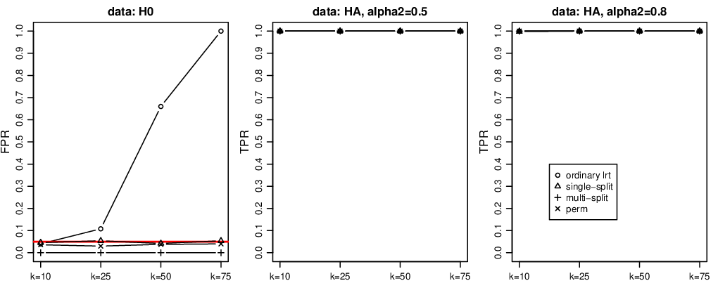
The values and control the strength of the alternative for the regression and network cases respectively: A larger value results in two regression models which differ more. On the other hand a larger signifies that the two networks have more edges in common and are therefore more similar. For each of the four settings we perform simulation runs for the null- and the different alternative hypothesis. We then compute for each run a p-value with the single- and the multi-split method (50 random splits, ). We compare the proposed methodology with p-values obtained using the asymptotic -distribution of the ordinary likelihood-ratio statistic. We call this latter approach ordinary likelihood-ratio test. Further we compare with a permutation test where we use the symmetric Kullback-Leibler distance between -regularized estimates as a test statistic. This permutation test uses 100 random permutations and further details are given in Appendix C. For each setting we evaluate the fraction of wrongly rejected null hypothesis (false positive rate) and the fraction of correctly rejected hypothesis (true positive rate) at a significance level of 5%.
Results are shown in Figures 3-6. The false positive rate (FPR) of the ordinary likelihood-ratio explodes in all settings already for medium numbers of covariates , respectively . We further see that the single-split method is not able to control the true positive rate (TPR) at the 5% level in settings 1-2. This is most probably due to the fact that the sample size is too small and consequently the asymptotic approximation of the null distribution is not accurate enough. The multi-split method is much more conservative and has lower FPR. This observation is in agreement with results shown in Meinshausen et al. (2009). As expected, the permutation test controls the false positive rate at the 5% level. Concerning the TPR (or power of the test) we find that single-splitting, multi-splitting and the permutation test perform well in most settings. Only with weak alternatives (setting 1 and 2 with ) the TPR decreases. Interestingly, the permutation test exhibits loss of power for large values of , whereas single- and multi-split display higher power than the permutation test for large but lower power for small . For completeness Figures 9-12 in Appendix D provide more insights on the single-split algorithm. These figures report results for settings 1-4 with respect to the sparsity and screening properties.
For setting 1 with we further examine the distribution of the p-values obtained using the single-split method and the ordinary likelihood-ratio test when varying the sample size . For every we use 100 samples in the screening step of the single-split method and the rest of the samples are used for p-value calculations. Results are shown in Figure 7. We see that p-values obtained from the single-split method are very well approximated by the uniform distribution function. Only in the scenario with the approximation is not accurate enough which is also reflected in a too large number of false positives.



4.2 Application to genomic data from cancer biology
We apply the multi-split method to real datasets from cancer biology. For differential regression we take data from Broad-Novartis Cancer Cell Line Encyclopaedia (CCLE) (http://www.broadinstitute.org/ccle/home). Barretina et al. (2012) use the data to predict anticancer drug sensitivity from genomic data. They describe that the histone deacetylase inhibitor panobinostat shows increased sensitivity in haematological cancers compared to solid cancers. As the response variable we take experimentally determined sensitivity to panobinostat and we use gene expressions of the genes showing highest Pearson correlation over all samples with panobinostat as the predictor matrix. We compare the three cancer subtypes with the largest sample size: lung cancer ( cell lines), skin cancer ( cell lines) and cancer with haematopoietic and lymphoid-tissue origin (abbreviated with haem, cell lines). For differential network we use data from The Cancer Genome Atlas (TCGA) data portal (http://www.cancergenome.nih.gov). We consider gene expression data of the genes present in the cancer gene list of Hahn and Weinberg (2002) (downloadable at http://www.cbio.mskcc.org/CancerGenes) and compare lung squamous cell carcinomas against colon adenocarcinomas.
For both examples we compute p-values with the multi-split method ( splits) and with the permutation test (500 permutations). In the differential regression example the sample sizes are very small and cross-validation in the screening step can lead to active-sets which are too large. Therefore, we adapt the screening step by setting the smallest coefficients to zero whenever there are more than non-zero coefficients ( denotes the sample size involved in the screening step). We further carry out “back-testing” by dividing data randomly into populations and and then performing significance testing. All results are shown in Table 1. In the regression example the multi-split method gives considerably smaller p-values than the permutation test. A potential explanation could be that the permutation test exhibits small power in difficult scenarios (see settings 1 and 2 in Section 4.1 with , i.e., right panel in Figures 3 and 4). In the differential network example both methods have p-values which are numerically indistinguishable from zero. For the permutation test this implies that the observed test statistic is always larger than those obtained from random permutations. All p-values obtained for back-testing equal one which is reassuring. Figure 8 shows histograms of all p-values obtained by the multi-split method and illustrates both the sensitivity of p-values to single splits and also the information contained in the entire distribution of p-values obtained in the iterative, multi-split approach. For example in the comparison of skin against haem we get the whole range of p-values between zero and one. However, the distribution of these p-values is heavily skewed towards zero which is reflected in an aggregated p-value of 0.022.
| multi-split | permutation | ||
| Diffreg | lung-skin | 1 | 0.918 |
| lung-haem | 0.040 | 0.464 | |
| skin-haem | 0.022 | 0.220 | |
| Diffnet | lusc-coad |

5 Discussion and conclusions
We have presented a novel and very general approach for high-dimensional two-sample testing. We combined ideas including sample-splitting, non-nested hypothesis testing and p-value aggregation to propose a methodology that allows two-sample testing for a wide range of high-dimensional models. We treated in detail linear regression (differential regression) and Gaussian graphical models (differential network) and validated their performance on simulated and real data.
Our methodology is supported by asymptotic theory. However, our results obtained in Proposition 2.1 and Theorem 2.1 do not reflect a truly high-dimensional setup as they consider the active sets selected in the screening step as fixed. An aim of our ongoing research is to generalize these results to the case where the size of the active sets can grow with a rate of smaller order than the sample size.
Whilst the focus of this paper was not on applications, we note that the methodology we propose should have immediate utility in biology. Differential network can be used to test a number of hypotheses of current scientific interest. For example, in cancer biology it is widely believed that genomic differences between cancer types and subtypes may in some cases be manifested also at the level of biological networks, including gene regulatory and protein signaling networks. However, we are not aware of existing methodology that allows such hypotheses to be tested statistically under the relevant conditions of moderate sample size and high dimensionality. Our approach can be used to test such hypotheses directly from high-throughput data, as illustrated in the example above. A further application of the differential networks formulation of our approach is in gene-set testing. Currently, gene set tests (e.g., Subramanian et al. (2005); Irizarry et al. (2009)) are not truly multivariate. Our approach could be directly applied to test differences in gene sets at the level of not only means but also covariances or networks.
Acknowledgements: The authors thank Peter Bühlmann for discussions. This work was supported in part by NCI U54 CA 112970 and the Cancer Systems Biology Center grant from the Netherlands Organisation for Scientific Research.
References
- Bai and Saranadasa (1996) Bai, Z. and Saranadasa, H. (1996) Effect of high dimension: By an example of a two sample problem. Statistica Sinica, 6, 311–329.
- Barretina et al. (2012) Barretina, J., Caponigro, G., Stransky, N., Venkatesan, K., Margolin, A. A., Kim, S., Wilson, C. J., Lehár, J., Kryukov, G. V., Sonkin, D., Reddy, A., Liu, M., Murray, L., Berger, M. F., Monahan, J. E., Morais, P., Meltzer, J., Korejwa, A., Jané-Valbuena, J., Mapa, F. A., Thibault, J., Bric-Furlong, E., Raman, P., Shipway, A., Engels, I. H., Cheng, J., Yu, G. K., Yu, J., Aspesi, P., de Silva, M., Jagtap, K., Jones, M. D., Wang, L., Hatton, C., Palescandolo, E., Gupta, S., Mahan, S., Sougnez, C., Onofrio, R. C., Liefeld, T., MacConaill, L., Winckler, W., Reich, M., Li, N., Mesirov, J. P., Gabriel, S. B., Getz, G., Ardlie, K., Chan, V., Myer, V. E., Weber, B. L., Porter, J., Warmuth, M., Finan, P., Harris, J. L., Meyerson, M., Golub, T. R., Morrissey, M. P., Sellers, W. R., Schlegel, R. and Garraway, L. A. (2012) The Cancer Cell Line Encyclopedia enables predictive modelling of anticancer drug sensitivity. Nature, 483, 603–607.
- Bühlmann (2012) Bühlmann, P. (2012) Statistical significance in high-dimensional linear models. arXiv.org: 1202.1377.
- Bühlmann and van de Geer (2011) Bühlmann, P. and van de Geer, S. (2011) Statistics for High-Dimensional Data: Methods, Theory and Applications. Springer Series in Statistics. Springer.
- Cai et al. (2011) Cai, T., Liu, W. and Xia, Y. (2011) Two-sample covariance matrix testing and support recovery in high-dimensional and sparse settings. Tech. rep., Department of Statistics, The Wharton School, University of Pennsylvania.
- Chen and Qin (2010) Chen, S. X. and Qin, Y.-L. (2010) A two-sample test for high-dimensional data with applications to gene-set testing. Annals of Statistics, 38, 808–835.
- Davies (1980) Davies, R. B. (1980) Algorithm AS 155: The distribution of a linear combination of chi-2 random variables. Journal of the Royal Statistical Society. Series C, 29, 323–333.
- Duchesne and de Micheaux (2010) Duchesne, P. and de Micheaux, P. L. (2010) Computing the distribution of quadratic forms: further comparisons between the Liu-Tang-Zhang approximation and exact methods. Computational Statistics and Data Analysis, 54, 858–862.
- Fan and Li (2001) Fan, J. and Li, R. (2001) Variable selection via penalized likelihood. Journal of the American Statistical Association, 96, 1348–1360.
- Friedman et al. (2008) Friedman, J., Hastie, T. and Tibshirani, R. (2008) Sparse inverse covariance estimation with the graphical Lasso. Biostatistics, 9, 432–441.
- Friedman et al. (2010) Friedman, J., Hastie, T. and Tibshirani, R. (2010) Regularization paths for generalized linear models via coordinate descent. Journal of Statistical Software, 33, 1–22.
- Hahn and Weinberg (2002) Hahn, W. C. and Weinberg, R. A. (2002) Modelling the molecular circuitry of cancer. Nature Reviews Cancer, 2, 331–341.
- Irizarry et al. (2009) Irizarry, R. A., Wang, C., Zhou, Y. and Speed, T. P. (2009) Gene set enrichment analysis made simple. Statistical Methods in Medical Research, 18, 565–575.
- Li and Chen (2012) Li, J. and Chen, S. X. (2012) Two sample tests for high-dimensional covariance matrices. Annals of Statistics, 40, 908–940.
- Lopes et al. (2012) Lopes, M., Jacob, L. and Wainwright, M. J. (2012) A more powerful two-sample test in high dimensions using random projection. arXiv.org:1108.2401.
- Meinshausen and Bühlmann (2006) Meinshausen, N. and Bühlmann, P. (2006) High dimensional graphs and variable selection with the Lasso. Annals of Statistics, 34, 1436–1462.
- Meinshausen et al. (2009) Meinshausen, N., Meier, L. and Bühlmann, P. (2009) P-values for high-dimensional regression. Journal of the American Statistical Association, 104, 1671–1681.
- Park and Hastie (2007) Park, M. Y. and Hastie, T. (2007) L1-regularization path algorithm for generalized linear models. Journal of the Royal Statistical Society: Series B, 69, 659–677.
- Subramanian et al. (2005) Subramanian, A., Tamayo, P., Mootha, V. K., Mukherjee, S., Ebert, B. L., Gillette, M. A., Paulovich, A., Pomeroy, S. L., Golub, T. R., Lander, E. S. and Mesirov, J. P. (2005) Gene set enrichment analysis: a knowledge-based approach for interpreting genome-wide expression profiles. Proceedings of the National Academy of Sciences of the United States of America, 102, 15545–15550.
- Tibshirani (1996) Tibshirani, R. (1996) Regression shrinkage and selection via the Lasso. Journal of the Royal Statistical Society, Series B, 58, 267–288.
- Vuong (1989) Vuong, Q. H. (1989) Likelihood ratio tests for model selection and non-nested hypotheses. Econometrica, 57, 307–333.
- Wasserman and Roeder (2009) Wasserman, L. and Roeder, K. (2009) High-dimensional variable selection. Annals of Statistics, 37, 2178–2201.
- Yuan and Lin (2006) Yuan, M. and Lin, Y. (2006) Model selection and estimation in regression with grouped variables. Journal of the Royal Statistical Society, Series B, 68, 49–67.
- Zou and Hastie (2005) Zou, H. and Hastie, T. (2005) Regularization and variable selection via the elastic net. Journal of the Royal Statistical Society, Series B, 67, 301–320.
Appendix A Proofs of Section 2
Without loss of generality, we take . We assume that the following assumptions (A1)-(A6) hold:
- (A1)
Data and are i.i.d. samples with drawn from some common density function and , . The conditional density function is strictly positive for almost all and all .
- (A2)
, and are compact subsets of , and the conditional density function is continuous in .
- (A3)
For almost all , is dominated by an integrable function independent of . The functions
have unique maximums on , and at , and .
- (A4)
For almost all : is twice continuously differentiable on ; and are dominated by integrable functions independent on .
- (A5)
If , then is an interior point of , and . Further, is a regular point of and .
- (A6)
The information matrix equivalence holds, i.e., for all we have:
Proof of Proposition 2.1 Given assumptions (A1)-(A3) and noting that , (a consequence of the screening property) we have
| (A.15) |
where is the standard Kullback-Leibler divergence. If , then at least one term on the right hand side of equation (A.15) is strictly positive. Therefore, under :
Proof of Theorem 2.1 Consider the setting in Vuong (1989) with competing models and , i.e.,
with , , and . If the screening property holds then model is correctly specified and the pseudo-true values equal the true values . Furthermore, if we have then the screening property guarantees that also is correctly specified and that . As a consequence we have . Therefore, assuming assumptions (A1)-(A5), it follows from Theorem 3.3 (i) in Vuong (1989) that
where and the weights are eigenvalues of the matrix
| (A.16) |
The matrices , , , , and are defined as in Vuong (1989). If we set
then we obtain as a consequence of the independence of the populations and :
and
By invoking the information matrix equivalence, assumption (A6), we find
Proof of Proposition 2.2 Set , , and The eigenvalues of are the solutions to the equation
Assume
If , then we find by using Schur’s complement
| (A.17) |
where . The second term on the right of equation (A.17) has roots. Therefore of the eigenvalues equal one. As , we can write
Solving
is equivalent to
| (A.18) |
An easy calculation involving Schur’s complement shows
Further, we find
Putting together, equation (A.18) reads
| (A.19) |
with
From (A.19) we deduce
and conclude that of the eigenvalues are zero and that the remaining eigenvalues are obtained by computing eigenvalues of
The proof for the case with works similarly.
Appendix B Derivation of equations (3.13) and (3.14) in Section 3
Equation (3.13)
Set and note that . We then find:
Equation (3.14)
Invoking formulas on fourth moments of a multivariate Normal distribution we find:
Appendix C Permutation test and symmetric Kullback-Leibler divergence
The symmetric Kullback Leibler divergence is defined as
Consider a random partitition of the data into two groups and . We construct a permutation test based on the test statistic
with
and tuning parameter chosen by cross-validation ().
For the regression model the Kullback-Leibler divergence equals:
For the Gaussian graphical model we have:
Appendix D Additional Figures of Section 4


