On finite-temperature holographic QCD in the Veneziano limit
Abstract:
Holographic models in the universality class of QCD in the limit of large number of colors and massless fermion flavors, but constant ratio , are analyzed at finite temperature. The models contain a 5-dimensional metric and two scalars, a dilaton sourcing and a tachyon dual to . The phase structure on the plane is computed and various 1st order, 2nd order transitions and crossovers with their chiral symmetry properties are identified. For each , the temperature dependence of and the condensate is computed. In the simplest case, we find that for up to the critical there is a 1st order transition on which chiral symmetry is broken and the energy density jumps. In the conformal window , there is only a continuous crossover between two conformal phases. When approaching from below, , temperature scales approach zero as specified by Miransky scaling.
1 Introduction
QCD in the Veneziano limit [1],
| (1.1) |
is expected to display a host of interesting and mostly non-perturbative phenomena, including:
- •
- •
It is expected that at a critical , the conformal window will end, and for , the theory will exhibit chiral symmetry breaking in the IR. This behavior is expected to persist down to . For the IR theory is a conformal field theory at strong coupling, that progressively becomes weak as .
- •
Near and below , there is the transition region to conventional QCD IR behavior. In this region the theory is expected to be “walking”: This means that the theory appears to be approaching the IR fixed point as the coupling evolves very slowly for many e-foldings of energies. But chiral symmetry breaking is nevertheless triggered and in the deep infrared the coupling diverges as in QCD. The slow evolution of the coupling has been correlated with a nontrivial dimension for the quark mass operator near two, rather than three (the free field value). IR observables are expected to obey the Miransky scaling [4, 5] as from below.
- •
New phenomena are expected to appear at finite density driven by strong coupling and the presence of quarks. These include color superconductivity [6, 7]. In this case, however, gauge invariant vevs are effectively double trace operators and the phase structure is determined at the next to leading order in .
The existence of the “walking” region makes the theory extremely interesting for applications in dynamical electroweak symmetry breaking (technicolor). This has also motivated an intensive lattice Monte Carlo work during recent years [8, 9, 10]. The bulk of this work has been done at zero temperature; recently there appeared the first attempts to go to finite for QCD with , up to 8 [11, 12, 10] and for non-QCD-like theories [13]. Chiral effective theories have also been applied [14, 15, 16, 17, 18, 19, 20, 21].
The aim of the present work is to study a class of holographic bottom-up models (V-QCD) that belong to the universality class of QCD with massless quarks in the Veneziano limit [22] at finite temperature and zero chemical potential. We will calculate the temperature dependence of the free energy density (= pressure = ) and of the quark condensate (). The former acts as an effective order parameter for deconfinement (at large ), for which there is no true order parameter associated with a symmetry.11 1 A related one, used commonly in lattice work, is the expectation value of the Polyakov loop. The quark condensate is a true order parameter for chiral symmetry if quarks are massless. The calculation is carried out for the full range of , .
Discontinuities or rapid variations in pressure (or energy density) and quark condensate can be used to define phase boundaries associated with deconfinement and chiral symmetry restoration temperatures and . We will use the usual nomenclature: If the th derivative of is discontinuous, the transition is of th order. We also consider continuous crossovers which are identified by using the scaled quantity . Its maximum defines the crossover temperature . The phase diagram is defined as a plot of all phase boundaries on the plane. The phase diagrams we present will also contain a rich structure of metastable states, namely local (but globally subleading) minima of the free energy.
In the holographic approach the thermal transitions will be transitions between various 5-dimensional black hole and “thermal gas” metrics and the nomenclature of transitions, explained later in great detail, will be correspondingly different. The holographic approach is constrained but not fully constrained and we cannot give a precise prediction of the phase diagram of hot V-QCD. We can state the most plausible behavior but we can also mention a few other alternatives. We will always find the analogues of and , but we will also find transitions with no obvious QCD interpretation. Whether these reflect real physics of hot QCD in the Veneziano limit or whether they are artifacts of the holographic approach will be an interesting problem for further study.
The usual expectation is that there is a 1st order line at ; in the large limit one can actually prove that [14, 15]. The main class of our predictions reflect these properties: for smaller we find that deconfinement and chiral symmetry restoration coincide, but for approaching the deconfining and chiral transitions can become separate so that (see, for example, Fig. 13 below). The chiral transition is then of 2nd order (and mean field type). Furthermore, for smaller the separate 2nd order chiral transition is in the metastable region so that it can be reached if the system is supercooled [23]. One might here add that for stable phases may be reached at large chemical potential [24, 25].
The starting point of our finite temperature analysis is the holographic model introduced in [22], based on previous theoretical ideas in [26, 27, 28, 29, 30]. Moving to finite implies studying black hole solutions of the action in [22]. A defining characteristic of this class of models is that they contain full backreaction between the duals of the color and flavor degrees of freedom. Earlier work [31, 32, 33, 34] on thermodynamics in such bottom-up models imposed quasiconformality directly on the beta function of the theory. One should note that walking behavior and the related “conformal transition” at have also been studied in top-down models [35, 36, 37, 38], as well as in simpler bottom-up models [39, 40] which do not attempt to model the backreaction. See also the review [41] on introducing backreacted flavor in the top-down models.
In this introduction we will first describe the special properties of V-QCD from [22] and then discuss general properties of its black hole solutions. Section 2 will contain a detailed discussion of the action of the model and of the two characteristic classes of scalar potentials. Section 3 presents the Einstein equations of the model, describes how they are numerically solved and, finally, how thermodynamics is computed from the numerical bulk fields. A particularly delicate issue here is the fixing of the quark mass to zero. We also briefly comment on fixing to some nonzero value. An extensive list of numerical results is given in Section 4. From these, the types of phase transition lines the models predict are determined. In Section 5, techniques for computing the condensate are described and several numerical results are given. One should note that this, as well as many other numerical issues in the model, are technically very demanding. Finally, Section 6 contains a discussion of what are the effects of making the quark mass nonzero. Several detailed considerations are collected in Appendices.
1.1 V-QCD at zero temperature
In [22] a class of bottom-up holographic models was introduced (named V-QCD) and shown to be in the universality class of QCD in the Veneziano limit at zero temperature and density. These were 5-dimensional models of two scalars coupled to gravity. One of the scalars, the “dilaton” , is dual to (the QCD gauge coupling constant, or more precisely the ’t Hooft coupling). The other scalar, the “tachyon” , is dual to the quark mass operator . The potentials and interactions were modeled along successful bottom-up models for YM, namely Improved Holographic QCD (IHQCD) [26, 27, 28] and the idea that string theory tachyon condensation describes chiral symmetry breaking [29, 30, 42].
The bulk action considered was
| (1.2) |
with the ’t Hooft coupling (exponential of the dilaton ) and the tachyon22 2 We have taken the tachyon to be real and diagonal in flavor space. action33 3 To find the vacuum (saddle point) solution we have set the gauge fields dual to the QCD currents to zero, as they are not expected to have vacuum expectation values at zero density. We have also suppressed the Wess-Zumino terms as they also do not contribute to the vacuum solution.
| (1.3) |
The pure glue potential has been determined from previous studies [27]. The tachyon potential must satisfy some basic properties determined by the dual theory or by general properties of tachyons in string theory: (a) To provide the proper dimension for the dual operator near the boundary (b) To exponentially vanish for . The function captures, among other things, the transformation from the string frame to the Einstein frame in five dimensions. The class of potentials that were investigated in [22] are of the form
| (1.4) |
In the Veneziano limit, the back-reaction of the flavor sector on the glue sector is fully included.
As with IHQCD, it was arranged that the theory is asymptotically AdS in the UV up to logarithmic corrections in the bulk coordinate. The function is such that the potential , when the tachyon has not condensed () has an extremum 44 4 The extremum may exist for all or may disappear at some small . No changes in the phase structure at zero temperature for these two cases were found in [22]. at a finite value . As we approach the Banks-Zaks region [2], , the value of approaches zero. Without the tachyon, , the equations of motion imply that also , i.e., is an IR fixed point. When the dynamics of is included, the system approaches but is driven away from it as long as (see Fig.7 of [22]).
The dimension of the chiral condensate was calculated in the IR fixed point theory from the bulk equations. It was found that it decreases monotonically with for reasonably chosen potentials. It crossed the value 2 at where corresponds to the end of the conformal window as argued in [43].
The lower edge of the conformal window lies in the vicinity of 4. Requiring the holographic -functions to match with QCD in the UV, we find that
| (1.5) |
where the bounds are not strict but hold approximately for potentials that have smooth -dependence in the UV.
There is also a phenomenological heuristic argument for the value , simply from counting degrees of freedom. At low chiral symmetry is broken and the massless degrees of freedom are Goldstone bosons. At large there are weakly coupled degrees of freedom. These numbers are equal for . Conformal window and the location of its edge was also discussed within holographic frameworks related to V-QCD in [44, 33].
Apart from , there is a single parameter in the theory, namely where is the UV value of the (flavor independent) quark mass. For each value of , the bulk equations were solved with fixed sources corresponding to fixed . The vevs were determined such that the solution is “regular” in the IR. The notion of regularity is tricky even in the case of IHQCD (pure glue), as there is a naked singularity in the far IR. For the dilaton this has been settled in [26, 27]. For the tachyon the notion of regularity is different and has been studied in detail in [30].
The regularity condition was implemented in the IR. After solving the equations from the IR to the UV (this was done mostly numerically), there is a single parameter that determines the solutions as well as the UV coupling constants and vevs, and this is a real number controlling the value of the tachyon in the IR. This number reflects the single dimensionless parameter of the theory.
For different values of and the following qualitatively different regions were found in [22]:
- •
When and , the theory flows to an IR fixed point. The IR conformal field theory is weakly coupled near and strongly coupled in the vicinity of . Chiral symmetry is unbroken in this regime (this is known as the conformal window).
- •
When and , the tachyon has a nontrivial profile, and there is a single solution with the given source, which is “regular” in the IR. The IR theory is a theory with a mass gap.
- •
When and , there is an infinite number of regular solutions with nontrivial tachyon profile, and a special solution with an identically vanishing tachyon and a nontrivial IR fixed point. The infinite number of solutions with nontrivial tachyon are classified by their number of zeros. The solution with the lowest free energy is the one with no zeros.
- •
When and , the theory has vacua with nontrivial profile for the tachyon. For every non-zero , there is a finite number of regular solutions that grows as approaches zero.
In [22] two large classes of tachyon potentials were identified. Potentials in class I, have constant in (1.4). In this case the tachyon diverges exponentially in the IR for the regular solution
| (1.6) |
where is a known constant (see Appendix B) and is the only integration constant controlling the solution. It determines the source (mass) in the UV. Potentials in class II, have as , and a tachyon that diverges in a milder way in the IR as
| (1.7) |
where again is known and is the single integration constant controlling the regular solution. The qualitative conclusions above and below were valid for both classes of potentials.
In the region where several solutions exist, there is a interesting relation between the IR value controlling the regular solutions, and the UV parameters, namely . This is determined numerically, and a relevant plot describing the relation between and at fixed is in Fig. 1.
The solutions are characterized by the number of times the tachyon field changes sign as it evolves from the UV to the IR. For all values of there is a single solution with no tachyon zeroes. In addition, for each positive there are two solutions55 5 As and are related by a chiral rotation by , we can take . which exist within a finite range , where the limiting value decreases with increasing , and one solution for . In particular, for large enough fixed , we find that only the solution without tachyon zeroes exists.
For , out of all regular solutions, the “first” one without tachyon zeroes has the smallest free energy. The same is true for , namely the solution with nontrivial tachyon without zeroes is energetically favored over the solutions with positive as well as over the special solution with identically vanishing tachyon, which appears only for and would leave chiral symmetry unbroken. Therefore, chiral symmetry is broken for .
In the region just below , [22] found Miransky scaling for the chiral condensate. As ,
| (1.8) |
For , let be the mass of the tachyon at the IR fixed point and the IR AdS radius. The coefficient is then fixed as
| (1.9) |
The behavior at and below the conformal transition at is to a large extent independent of the details of the model. In particular, no information on the nonlinear terms in the tachyon EoM is needed or how the IR boundary conditions are fixed. In the same region, “walking” of gauge coupling is realized. The YM coupling flows from small values to values very near , remains approximately constant for many e-foldings of energy (in this regime the tachyon remains small), and then runs off to infinity, driven by a large value of the tachyon field in the IR. The walking is related to a long section of the solution which is similar to the one studied in earlier bottom-up models for walking [39].
The finite temperature analysis of V-QCD amounts to studying all black hole solutions with appropriate boundary conditions. To start with, any zero temperature solution becomes a candidate saddle point at finite temperature by compactifying time on a circle of radius . Any other competing black hole solution must have the same boundary conditions as well as a regular horizon in the IR.
As the dilaton always has a nontrivial UV source, it will always have a nontrivial profile in the black-hole solutions. With the tachyon, things can be different. In the massless case, its source is zero. Therefore there are two possible options (as in the zero temperature configurations discussed above): either it is identically zero (if the vev is also zero) or it is non-zero (implying a non-zero vev).
Therefore we have two large classes of black holes in the massless case: those with and those with . We will first consider the tachyon-free class.
1.2 Black holes without tachyon hair
If , we have black holes in a single scalar theory, with potential from (1.4). This is a potential with an extremum for 66 6 The extremum may also exist only for above some fixed , see the discussion further below. and no extremum when .
Black hole solutions for such potentials were discussed in generality in [27]. After fixing all invariances, they are characterised by a single IR constant, , the value of the dilaton at the horizon. The plot relating the temperature to contains important information about the thermodynamics of such black holes. Small values of denote large black-holes whereas larger values of correspond to smaller black holes (smaller horizon size and entropy). In all plots of this paper, dilatonic black holes without tachyon hair are denoted by red lines in the respective -diagrams, and we shall call the corresponding function .
When , can become arbitrarily large at zero temperature, implying that can also be arbitrarily large for the finite temperature configurations. At finite temperature there are two branches: large black holes which are stable and small black holes which are unstable. If the black-hole thermodynamics is stable, otherwise it is unstable. There is a minimum temperature above which such black holes exist as shown, for example, by the black line in Fig. 22 (left or right).
When , we have two possibilities. The first is that the potential has an extremum at for all , with and . The second is that such extremum only exists for , where . We shall denote these potentials with a star subscript.
At finite temperature, and when the potential has no extremum, the black hole without the tachyon hair exists for all positive . For the potentials studied here, function is qualitatively similar to the YM case () [27]. As shown in Fig. 17 (top-left) and in Fig. 19 (left), there are two black hole branches, which exist above some minimum temperature. The branch at low is thermodynamically stable, while the large- branch is unstable.
When the extremum is present, . The temperature of the black-hole corresponding to is , while that of has . There is no minimum temperature here. For any temperature there is always at least one black-hole solution. There are several possibilities that are shown as red lines in Figs. 7 (left), 9 (top), 10 (left) and 12 (left).
When is large, but still smaller than , the relation is one-to-one but contains a bump (a change of concavity) like in Fig. 9 (top). Then this is accompanied by a crossover behavior, signaled by a bump in the trace of the stress tensor , (aka interaction measure) as shown in Fig. 9 (bottom-right).
At low enough , the relation is not always one-to-one, as can be seen in Fig. 10 (left) or in Fig. 22. Then there are points where . In such a case there can be a first order transition between the stable branches of the black hole solutions. This is a remnant of the deconfining transition at (pure YM). In Fig. 22 both left and right several curves in the -plane for different indicate the successive structure of dilaton black holes (red lines). The black line corresponds to the pure YM () limit.
When we are in the conformal window. The only black holes that exist here are those without tachyon hair. The relation is monotonic and there is a continuous transition to the black-hole phase at , as in the AdS case in the Poincaré patch. The thermodynamic functions, especially the interaction measure, show a crossover maximum at a temperature that is moving towards the UV as .
1.3 Black holes with tachyon hair and zero quark mass
When we have black holes in the two scalar theory. The tachyon starts as near the UV boundary as the source (quark mass) vanishes. In all plots of this paper, such black holes (with both dilaton and tachyon hair) are denoted by blue lines in the respective -diagrams, and we shall denote the corresponding functions by . They are still one parameter solutions and can be parametrized again by the value of at the horizon, which translates into the temperature. These black holes usually exist for all and our discussion below focuses in this region.
Because the presence of the nontrivial tachyon perturbs and annuls the possible nontrivial IR fixed point, for such black-holes, can take arbitrarily large values. This can be seen from the blue lines in Figs. 7 (left), 9 (top), 10 (left) and 12 (left). For all such black holes, the chiral condensate is determined by the regularity of the black hole solution. It decreases as decreases, and at some point it vanishes. At this point, the blue line in the ()-diagram merges with the red line corresponding to a that we call throughout the paper. This can be seen in all the figures mentioned above.

The shape of the blue line can vary as a function of and the type of potential. There are three typical examples of shapes:
- •
Simple lines that are monotonic as the one depicted in Fig. 12 (left). This is an example of a monotonic blue branch where all such black-holes are thermodynamically unstable. Moreover, they have a minimum temperature. In such a case, they can never be thermodynamically dominant. At some temperature the vacuum thermal solution is dominated by a dilaton black hole on the red line, and the chiral restoration transition is 1st order.
- •
Lines with two branches as the one depicted in Fig. 10 (left). Here the blue line has two parts one (to the left) that is thermodynamically stable and another to the right that is thermodynamically unstable. In such a case, the system is in the thermal vacuum solution at low enough temperatures, then jumps with a 1st order transition to the tachyon-hairy solution (the part of the blue line that is thick in Fig. 10 (left)) which still break chiral symmetry, and then eventually smoothly transits to the red line at the point where the blue and red lines merge, via a chirally-restoring 2nd order transition.77 7 It may also happen that the thermodynamically stable branch is only metastable, in which case the system jumps directly to the black hole branch without tachyon hair, and chiral symmetry is thus restored at this 1st order transition. The more complicated branch structure discussed in the next bullet may similarly contain metastable branches.
- •
Lines with more than two branches as the one depicted in Fig. 11 (left). In this example the blue line has four branches, two unstable and two stable. There are in total three phase transitions here, first from the vacuum thermal solution to the rightmost blue thick branch, then to the intermediate thick blue branch and finally a 2nd order chirally restoring transition to the red branch at the point they touch. In this case there are two 1st order transitions between three chirally breaking phases, and a 2nd order one to the chirally symmetric phase.
A concrete overall view of the dependence is presented in Fig. 2, in which is plotted for potentials of type II with SB normalisation (definitions specified later) for various . One sees clearly how the pure (black) YM curve is approached for . The thick curves represent stable phases; when a thick curve ends, the system makes a 1st order transition to the low phase. When thick curves change from red to blue curves, a 2nd order transition to a chirally broken phase takes place. For a more accurate picture of small , see Fig. 22.

1.4 The phase structure of different V-QCD models
There are three main ingredients that characterize a priori different QCD models which, however, have the same phase structure and qualitative behavior at zero temperature:
- •
The asymptotics of the tachyon solution in the IR. This is controlled by the behavior of the function in the tachyon potential in (1.4). When is constant, the tachyon diverges exponentially in the IR, and we call such potentials of type I. When diverges as in the IR ( large) then the tachyon diverges as a square root in the IR, and we call such potentials of type II.
- •
For any potential, the UV constant factor of in (1.4), defined in (2.22) can vary in finite range, which in appropriate units is , as in (2.30). We pick for each type of potential three indicative values of that in general might give different physics, namely , , and .88 8 Notice that the exactly zero value of is actually excluded, because it predicts wrong anomalous dimensions for quark mass or the chiral condensate [22]. We anyhow consider it as the limiting case of the allowed solutions. Moreover, may exceed the upper limit of , if dependence is allowed. We also consider -dependent value, specified in (2.32) that corresponds to the normalization of the UV degrees of freedom of the free energy to the Stefan-Boltzmann limit of QCD.
- •
A final variation can be obtained on all of the above by using a glue potential in (1.4) that has
(a) an extremum for all in the appropriate range, .
(b) an extremum only in part of this range, . We will denote the potentials in this case by a star subscript.
According to the above options PotI denotes a potential in the type I class, with and an IR critical point that exists only down to a finite .
Let us then summarize the phase structure of the model as and the temperature are varied (at zero quark mass). In general one expects the phase diagram of Fig. 8, so that for there is the 1st order transition at finite temperature, which also separates the chirally symmetric and broken phases. For the low temperature and high temperature configurations correspond to a tachyonless black holes, and, one expects a continuous crossover between these two.
For the various potentials presented above, this phase diagram is indeed obtained in the zeroth approximation, but for there are additional details which depend on the choice of potentials as follows.
- •
For potentials I the phase structure depends strongly on the choice for (see Fig. 18). For the lowest value , there is only one 1st order transition at99 9 in Fig. 18. for all , except possibly for very close to , where solving the phase diagram numerically becomes demanding. As is increased, a complicated structure appears near , where we have two 1st order transitions between chirally broken phases, and the restoration of chiral symmetry at a 2nd order transition at even higher temperature. At even higher the 1st order transitions combine again into a single one, but the separate 2nd order transition continues to exist for close to . At low , there is also a surprising change as increases. The chiral symmetry breaking phases disappear, but there is a 1st order transition between two chirally symmetric black hole phases at a finite temperature instead.
- •
For potentials II the dependence on is milder (see Figs. 13 – 16). At high , for low up to some value , there is only the 1st order transition at1010 10 of Figs. 13 – 16 when it is in the stable brach. . When , the chiral symmetry restoration takes again place at a 2nd order transition at such that . For decreasing , increases, and finally disappears by joining with .
- •
For the potentials I∗, the phase structure is the standard one for high , i.e., a 2nd order transition and a 1st order one with critical temperatures within a range , with the former separating the chirally symmetric and broken phases (see Fig. 19). For lower there is only one 1st order transition. For , in the region where the effective potential does not admit an extremum, chiral symmetry is intact at all temperatures. We find a single 1st order transition between chirally symmetric thermal gas and black hole phases.
- •
For potentials II∗, the phase structure is simple (see Fig. 17): there is a single 1st order transition for all . In particular, the system is in a chirally broken phase at low temperatures, even in the region of low where the effective potential does not have an extremum.
2 Defining V-QCD
2.1 Gravity action of the model
The action of V-QCD is [22]
| (2.10) |
where1111 11 Notice that for notational simplicity we have absorbed a factor of , which is visible in Eq. (1.3), into . See also Eq. (2.19) below.
| (2.11) | |||||
The metric Ansatz is
| (2.12) |
and the two scalar functions, sourcing and sourcing , are
| (2.13) |
In the second form has been factored out of the DBI action. The Gibbons-Hawking counter term would be
| (2.14) |
with, for a hypersurface const,
| (2.15) |
Notice also that we have set the gauge fields , which are dual to the left and right handed fermion currents, to zero, and neglected the Wess-Zumino terms. These terms do not affect the thermodynamics of the models.
The background solution of the dilaton and the warp factor are identified as the ’t Hooft coupling and the logarithm of the energy scale of the dual field theory, respectively [26]. As a matter of convention, we shall fix the normalisation of so that its relation to the perturbative QCD coupling is
| (2.16) |
The results of the model are independent of this normalisation, changing one simply has to change the potentials by . The convention of [22], for example, is obtained by shifting by .
Important ingredients of the model are the relation of the bulk fields at to the QCD beta and quark mass anomalous dimension functions evaluated for a coupling at scale . Motivated by the connection to field theory, one defines
| (2.17) |
Matching with the perturbative expansion of the QCD beta function gives
| (2.18) |
The action contains the gluonic potential and the fermionic potential , which will be specified to the form
| (2.19) |
The detailed form of these and the functions will be discussed in the following subsections.
2.2 Construction of the potentials
The potentials can be constructed in stages. First one fixes the potentials and up to order in the UV, using the two scheme independent coefficients of the beta function. This analysis is simplified by the fact that the tachyon decouples in the UV. Next one fixes the UV behavior of the functions and , which parametrize the tachyon dependence of the action using the similarly scheme independent UV running properties of the quark mass and the condensate. Finally, one fixes the large behavior of the potentials by requiring that the model reproduces known features of QCD in the IR, such as confinement, linear Regge trajectories, and reasonable zero-temperature phase structure. We shall discuss the various steps in detail below (see also [22]).
2.2.1 The potentials from the beta function in the UV
In the UV, since the tachyon vanishes much faster than the dilaton, we can first set it to zero. Then the dilaton profile can be linked to the effective potential [22] by using Einstein’s equations [26]. Defining , to order ,
| (2.20) | |||||
| (2.21) | |||||
| (2.22) |
where we expanded
| (2.23) |
and where we have introduced an dependent AdS radius
| (2.24) |
Applying equation (2.21) for we have for the gluonic potential
| (2.25) | |||||
| (2.26) |
where are the values of for and . In practice, one usually sets the (dimensionful) quantity .
By using equations (2.21) and (2.22) one can now solve for the coefficients of the fermionic potential:
| (2.27) |
| (2.28) |
| (2.29) | |||||
These equations still involve one free parameter, which can be taken to be either or . We shall study two ways to fix this parameter. First, we can take to be constant. In this case [22]
| (2.30) |
and the -dependent AdS radius is given by
| (2.31) |
Second, we can make a special -dependent choice, which (as we shall show later) automatically normalises the free energy at large to Stefan-Boltzmann:
| (2.32) |
Further, we have to fix the dependence of the functions and in the tachyon part
| (2.33) |
of the action, where . The leading logarithmic term to the UV expansion of the tachyon should be (remember that the energy dimension of is )
| (2.34) |
to satisfy the scheme independent UV running of the quark mass. Here is the leading coefficient of the anomalous dimension of the quark mass in QCD, . By using the tachyon equation of motion one sees that this requires that for small ,
| (2.35) |
2.2.2 Large behavior of the potentials
To specify the full potential we have to continue the small expansions to large . The guideline is quark confinement and chiral symmetry breaking at small and the appearance of an infrared fixed point at some (see [22]). Since there is no unique path to the result, we present the final forms of the potentials we use and motivate them.
We use the gluonic potential
| (2.36) |
which is constructed from the expansion (2.25) by simply multiplying the term by the confinement factor
| (2.37) |
Then has the proper large- behavior [26] but the small- behavior is left intact. One could add scale factors of type containing more parameters.
For the fermionic potential in
| (2.38) |
we consider two different choices. The first one is obtained directly using (2.27)-(2.29)
| (2.39) | |||||
Here one could as well use the parameter which is related to by
| (2.40) |
For this choice the effective potential
| (2.41) |
has a single maximum at finite positive for all , indicating a (possible) infra-red fixed point.
The second choice is obtained introducing the confinement factor (2.37) also for the fermionic potential, i.e.,
| (2.42) | |||||
Now the effective potential has a maximum only at large . To see this concretely, consider again the case (2.32). The asymptotic large- behavior of now is times the function
| (2.43) |
This function is positive for small , negative at large () and has a zero at . Thus there is a (possible) fixed point only for .
Let us then discuss the IR behavior of the potentials and which appear in the tachyon DBI action. For the function we will consider the large- asymptotics
| (2.44) |
This is motivated by the fact that in the action the combination has the same asymptotics as at large , where is the metric factor in the string frame. To ensure that the fractional exponent limit at large does not spoil analyticity at small , we replace by in the expression for .
More precisely, two qualitatively different, acceptable choices for the IR asymptotics of (and ) were identified in [22]. These are produced by the following two choices. The first choice has
| (2.45) |
and leads to tachyon growing exponentially at large ,
| (2.46) |
where is a known constant (see Appendix B) and parametrises the solutions. The second choice is given by
| (2.47) |
and for them the leading divergence is
| (2.48) |
where the constant is again known and now parametrises the solutions. To select this solution, it is required that the last term in the square brackets in (2.47) grows faster than .
Finally, let us summarize our choices for acceptable potentials. We always keep fixed to the expression (2.36) and choose , , and as follows:
- •
- •
- •
- •
Potentials II∗: We use with the confinement factor, but use the other choice (2.47) for and . Then the fixed point exist only for large , and the tachyon diverges as in the IR.
To fully pin down the potentials, we also need to specify the value of (or ) which is used. We choose four reference values:
- •
(and constant). This is the lower bound of . Actually, exactly zero is not acceptable because the anomalous dimensions of the quark mass and the chiral condensate do not sum up to zero. This case is nevertheless interesting as it is the limit of acceptable solutions.
- •
. This is the standard choice studied in [22].
- •
. For constant , this is the largest possible value, for which as .
- •
An ongoing work [45] studies the meson spectra in this model. As it turns out, the potentials I and I∗ admit linear “Regge” trajectories, so that the quadratic masses are asymptotically linear in the excitation number, , independently of the other quantum numbers. Potentials II and II∗, however, have linear trajectories only in the glueball sector, while the other trajectories are quadratic, . As linear trajectories are expected in QCD, this observation favors potentials I and I∗.
2.2.3 IR fixed point and the BF bound for the tachyon
Now that the potentials are defined, one can check that they satisfy an important requirement: they permit the determination of the bulk dilaton mass and, equating this with the Breitenlohner-Freedman (BF) instability bound, the determination of the start of the conformal window. Take (there is no chiral symmetry breaking in the conformal window) and note that at small , . However, grows faster and the conformal window starts at the value defined by the vanishing derivative
| (2.49) |
Given one defines an IR AdS radius
| (2.50) |
The tachyon mass at in units of becomes
| (2.51) |
Gravity solutions with are stable when ; the conformal window thus starts when (2.51), as a function of , has the value 4.
| PotI | PotI∗ | PotII | PotII∗ | |
|---|---|---|---|---|
| 4.10209 | 4.33334 | 4.17825 | 4.38493 | |
| 3.99591 | 4.33334 | 4.07968 | 4.38493 | |
| 3.71607 | 4.33334 | 3.80086 | 4.38493 | |
| SB | 3.59172 | 4.33334 | 3.70008 | 4.38493 |
Eq. (2.51) can be evaluated for the two choices of above. For the choice (2.45) (types I and I∗) the equation becomes
| (2.52) |
For the choice (2.47) (types II and II∗), the -equation (2.51) has the form
| (2.53) |
The values of can then be calculated by inserting the potential and the chosen value for in these equations. The critical values for the potentials listed above are given in Table 1.
The -dependence of the tachyon mass for all the potential choices suggested above is shown in Fig. 3. The critical value is the rightmost point where the curve intersects the horizontal dashed line where the BF bound is saturated. For potentials I∗ and II∗ (solid magenta curves) the fixed point only exists for with . In this case the tachyon mass diverges as approaches from above.
From (2.52) and (2.53) one sees, using the asymptotics of the potentials (see Eq. (4.99) below), that for type I and for type II as . They thus behave completely differently in this limit, for type I the mass vanishes, for type II it grows without bounds. In particular, for potentials I and for low the (absolute value of the squared) tachyon mass dives below the BF bound. This means that the existence of a solution with a nontrivial tachyon profile and zero quark mass is not guaranteed [22], which means that chiral symmetry could remain intact even at low temperatures. However, in most of the cases, such a solution anyhow exists all the way down to , and the expected picture with chiral symmetry breaking is obtained. We shall discuss this issue in more detail below.


3 V-QCD at finite temperature: equations and their solution
The V-QCD action has two kinds of vacua at finite temperature, either with identically vanishing tachyon or with nontrivial tachyon profile. The tachyonless black hole solutions can be constructed in the same way as in the Yang-Mills case [27]. Below most of the discussion will in principle assume the presence of the tachyon, but the construction for the solutions without the tachyon can be obtained simply by setting everywhere.
3.1 Equations and numerical solution
The goal now is to find numerical solutions of the Einstein’s equations for the metric functions and the scalars , satisfying
| (3.54) |
where marks the location of the horizon.
Due to the singular behavior of the solutions near the UV boundary (), it proves to be convenient to use as a coordinate instead of in the numerical solution. Carrying out this transformation, one finds that the combination
| (3.55) |
appears naturally. This is just a rewriting of the superpotential
| (3.56) |
The equations of motion then become
| (3.57) | |||||
| (3.58) | |||||
| (3.59) | |||||
| (3.60) | |||||
Here the prime denotes differentiation with respect to . Near the UV boundary ,
| (3.62) |
The range of thus is , where is the horizon,
| (3.63) |
Numerical integration starts by solving from the four first ones in terms of lower derivatives; the fifth equation, the equation for , will be used as a check and constraint. For brevity we introduce two square root factors:
| (3.64) |
and
| (3.65) |
The equations to be solved numerically then are
| (3.66) |
| (3.67) |
| (3.68) |
| (3.69) | |||||
In the equation the minus branch has to be chosen as is a monotonically decreasing function of . The derivatives are with respect to . The equations are autonomous in the sense that there is no explicit dependence. Numerical integration then proceeds as follows:
1. Let us fix the horizon at , where is a sufficiently small number, e.g., . the values of the functions at , which is taken as the initial value of numerical integration, are computed by using the expansions (B.140)-(B.143) in Appendix B. These numbers can now be obtained by inserting the values of . Among these the horizon values of the scalars, , remain as parameters, can be given an arbitrary positive value, +1, say. One then finds a solution valid from to some large upper limit by using NDSolve of Mathematica. The spatial coordinate can then, if needed, be computed by similarly integrating the differential equation
| (3.70) |
with the initial condition .
2. The so obtained first-level solution is scaled to one in the UV () by writing . Simultaneously , which is needed since Eq. (3.57) demands that be invariant. Finally, .
3. The final scaling is performed to guarantee that all solutions use the same unit of energy or, equivalently, have the same integration constant in the integral of the definition (2.17) of the beta function. This implies
| (3.71) |
where is the integration constant. By inserting the UV expansions of and from Appendix A, we identify . We wish to scale to one1212 12 After this, all quantities are expressed in units of ; omitting the factor would give a unit of energy depending on , and therefore define
| (3.72) |
and shift solutions by . In practice, one implements this by determining, for a given numerical solution (the term is optional),
| (3.73) |
and then performing the scaling
| (3.74) |
etc. for all the functions at level 2. The set , parametrised by the values of , is the final numerical solution. Note that the horizon has now been shifted to
| (3.75) |
at level 2 it was defined by .
3.2 Physical quantities
The set of functions (leaving out the index 3) can now be converted to various physical quantities:
The temperature is
| (3.76) |
and the value of at the horizon is
| (3.77) |
The quark mass is defined by the UV expansion of the tachyon:
| (3.78) |
so that, using the relation (3.71),
| (3.79) |
In practice, the extrapolation to can be carried out by measuring , as defined by the right hand side of Eq. (3.79), at two large values of and then linearly extrapolating to :
| (3.80) |
Linear extrapolation is chosen, because the leading neglected terms in the expansion of Eq. (3.79) are (up to logarithmic corrections) linear in .


3.3 Fixing quark mass
The above is for fixed . The really demanding task is to find the field configurations at fixed . For this one needs the curves . The quark mass is determined by the UV behavior of the tachyon: . To fix at fixed we have to solve the equations of motion at various and find that value of which leads to the desired UV behavior of .
3.3.1 Zero quark mass
In particular, we are interested in . This case splits in two parts: either identically (chiral symmetry holds) or nonzero (chiral symmetry broken).
If , solutions with are obtained simply by setting above. The solution is then controlled by the effective potential . For classes I and II, this increases monotonically from , but since grows faster, the derivative decreases and becomes finally zero at some (see Eq. (2.49)). The extremum of the potential marks the location of the IR fixed point, which is screened by the horizon at finite temperature. Indeed, the tachyonless black holes have , and for very close to we obtain configurations where the dilaton is approximately constant, for a long range of the coordinate before the horizon is reached in the deep IR.
For classes I∗ and II∗, the effective potential does not have an extremum for below . In this case the fixed point is absent, and the tachyonless black hole solutions are qualitatively similar to Yang-Mills () [26]. In particular can take any value.
For non-zero , the discussion of configurations has to take into account the existence of Efimov zeroes, oscillatory behavior when approaching , which was discussed above in the introduction. We discuss here the standard picture which is seen in most cases for . A rough description of more complicated cases is given in Appendix C. The situation is summarised in Fig. 5. For large , decreases monotonically from towards and ends with positive . We evaluate using (3.80) with two large values of (corresponding to a small UV cutoff in the -coordinate). When is decreased, ultimately an (approximate) configuration ( in Fig. 5) with monotonically decreasing is obtained.
This defines the curve in Fig. 6. One finds that these solutions are possible only if is larger than a fixed positive value, which we call . Decreasing further, first develops a zero so that . Continuing even further we find a second location where vanishes. This is a configuration with one tachyon node ( in Fig. 5). The pattern continues with an ever increasing number of nodes, until one ends up with the curve , below which a solution with the standard UV boundary does not exist. Numerically, the curves and can be separated, but already would require so much effort that we have not embarked on computing it. As we approach the conformal window, the curves get closer and closer to and finally vanish for .
We expect that increasing the number of nodes increases the free energy so that to study equilibrium states it is enough to compute . This was checked at zero temperature in [22] numerically for potentials I, and analytically in the limit as well as in the limit of large number of tachyon nodes.


3.3.2 Nonzero quark mass
For nonzero quark mass the special solution with identically vanishing tachyon profile is missing. However, there are solutions of various types for , as suggested by Fig. 5. We shall here restrict to the “standard” solutions which have monotonic tachyon, i.e., the region above in Fig. 5 (left). Below this curve there can be Efimov type solutions where the tachyon has nodes. As for , we expect that these solutions have higher free energies than the standard one. In the region of standard solutions, the dependence of quark mass is smooth (see Fig. 6). We have found numerically that for fixed the correspondence between and is one-to-one. Therefore can be kept fixed by following a set of well-defined curves on the ()-plane, some of which are sketched in Fig. 6.
It is also interesting to notice how the solution is obtained from the ones having finite quark masses as . What happens for nonzero quark mass is shown in Fig. 6 for a concrete computation. If (and fixed), the curve approaches zero as , indicating that approaches the chiral symmetry conserving solution () uniformly. If , approaches instead, which implies that converges to the standard chiral symmetry breaking solution .

3.4 Thermodynamics
We now want to compute minus free energy density or pressure of the gravity dual, assuming that all the quarks have the same mass . In particular, we are interested in . The chemical potential is zero, there is an equal number of quarks and antiquarks. The equilibrium phase has the largest pressure.
The basic strategy is to compute the temperature and entropy density from the formulas
| (3.81) |
where and are obtained by solving Einstein’s equations. The pressure is then obtained by integrating . The key technical issues are keeping track of the quark mass and specifying the integration constant in the pressure integral.
The general structure of temperature (for a case containing a fixed point) is shown in Fig. 7, to be consulted in association with Figs. 5 and 6. For two branches separate. Firstly, for there is the temperature computed for chirally symmetric vanishing tachyon solutions. We shall use the notation for this temperature below.
The chiral symmetry breaking solution exists for and as , the corresponding temperature curve ends precisely on the curve which has identically vanishing tachyon. The temperature curve is computed by using the zero node zero mass curve in Fig. 5. We shall use the notation for this temperature. If we computed the temperature for the one node solution , we would get a curve which lies significantly below the zero node curve in Fig. 7 and again ends on the zero tachyon curve. These solutions will have a higher free energy and we can thus neglect them.
Whenever the quark mass is nonzero, the tachyon cannot be vanishing and that branch disappears. However, as seen from Figs. 6 and 7, the small-mass curve very closely approximates the zero tachyon curve, also at small .


Analytic approximations are often useful. In the UV so that
| (3.82) |
Similarly, in the IR (see (B.131) in Appendix B),
| (3.83) |
For a numerical check, see Fig. 7. The interesting physics takes place in the region connecting these two limits.
The function decreases monotonically while the function decreases in the UV but starts increasing in the IR. The physics of the UV increase is obvious, this is the weak coupling limit which naturally corresponds to large of a thermal fluid. The (extremely slow) increase in the IR is a quantitative fact but does not correspond to a stable phase. This is simplest seen by computing the sound velocity
| (3.84) |
A stable phase has (equivalently, has a positive specific heat) and this requires . Thus only the UV decreasing part can correspond to a stable phase, the IR part is the unstable small black hole region, small since there. It is, nevertheless, crucially important for the phase structure.
To compute the pressure, we have to integrate the entropy density (3.81) over . Taking as a variable, we have integrals over the two branches in Fig. 7:
| (3.85) | |||||
| (3.86) |
where refer to the chiral symmetry broken ( and chirally symmetric (or unbroken, ) phases. The continuity of pressure at leads to a rather remarkable consistency check of the entire scheme: it demands
| (3.87) |
However, the difference on the RHS is nothing but the difference between the free energies of the broken and symmetric phases at :
| (3.88) |
This difference was computed in [22] from the solutions, with no black hole. Here they are computed in (3.87) from the black hole solutions and we have checked numerically that the results agree within the numerical precision.
The computation of the free energy now proceeds as follows, first for the simple structure of in Fig. 7:
- •
- •
At move to the chirally symmetric branch and fix the constant by demanding continuity of pressure. Since now , starts increasing. At first is still negative and the stable phase is the thermal gas phase with .
- •
At some pressure passes through 0. This defines a transition temperature since from now on the black hole metric has the largest pressure. Since this black hole phase is chirally symmetric.
- •
The latent heat of the transition is
(3.89) where the maximum value is obtained taking normalisation from (3.92) and using the UV approximation (A.121). Counting degrees of freedom one has Goldstone bosons in the low phase (for which we do not have a dependent gravity dual) and degrees of freedom in the high phase. These are equal at and if latent heat is naively assumed to be proportional to the jump in the number of degrees of freedom, one might rather expect to decrease when increases.
- •
Asymptotically, for large , we have so that
(3.90) If one for large assumes that the system becomes a gas of non-interacting bosons and fermions one should have
(3.91) This is obtained from (3.86) if
(3.92) which can be used to normalise the pressure.
- •
The above was for the simple in Fig. 7. Depending on the potentials, more complex structures can appear, as analysed in the following section.
- •
To present results for we choose to normalise it so that it approaches at large the ideal gas Stefan-Boltzmann pressure according to (3.91). However, we have no dynamical argument for fixing the dependence of in (3.92). We shall present the phase diagrams for two choices, for the automatically SB-normalised case (see Eq. (3.92))
(3.93) and for the fixed case
(3.94) In the former case one simply has
(3.95) and in the latter case1313 13 Notice that in this case the glue part of the V-QCD action will also depend on through the normalization factor .
(3.96) the factor is furthermore often implied, i.e., results for are given.


4 Results for the phase structure
4.1 Phase transitions
Let us first review what one qualitatively expects for the phase structure of V-QCD when the number of (massless) fermions is changed [46]. This is shown in Fig. 8, where the transition temperature between a low and a high phase is plotted as a function of .
A few reminders are in order. In the absence of quarks, YM has a center symmetry that is central in the definition of the confined and deconfined phases. The relevant order parameter is the Polyakov loop that transforms nontrivially under . If its expectation value is zero, we are in the confined phase, while the expectation value becomes non-zero in the deconfined phase.
This expectation value is simple to calculate holographically, [47]. It corresponds to a string world-sheet along the time circle, and hanging down straight in the holographic (radial) direction. The important difference is where it ends. At zero temperature, this worldsheet extends to and is the world-sheet of a free quark. Standard renormalization subtracts its contribution completely and therefore the Polyakov loop vev is zero (to leading order in ) in the zero temperature phase.
In a regular black-hole phase, the worldsheet terminates at the horizon and after subtraction the Polyakov loop expectation value is non-zero. This is in agreement with the identification of black-hole phases generically as deconfined phases.
In the presence of massless quarks, the center symmetry is not a symmetry any more, and the Polyakov loop is not an order parameter. However at large , there is alternative order parameter for a deconfined phase, namely the dependence of the free energy, . In the confined phases while in deconfined phases, . Again, with this criterion, the vacuum solutions (without horizons) are “confining” () while any black hole solution with regular horizon is “deconfined” (). It is therefore natural to use this criterion in our analysis in order to define deconfined phases.
The true symmetry in the case of massless quarks is chiral symmetry. This always has an order parameter, the chiral condensate, that distinguishes chirally symmetric from chirally broken phases.
Given the remarks above, we summarize what we would expect.
- •
For one has the Yang-Mills 1st order phase transition between a confined and deconfined phase. In the high deconfined phase, the symmetry is broken.
- •
For a somewhat higher one expects that there still is a 1st order transition. However, now this transition will involve chiral symmetry breaking/restoration.
- •
For approaching one expects the transition temperature to decrease rapidly as follows from Miransky scaling.
- •
For in the conformal window, , both the low and high phases are conformal ones, which can be separated by a crossover. The only transition happens at like in the AdS black hole in Poincaré coordinates.
The models we consider contain the full fermion backreaction and therefore predict a somewhat more detailed phase structure. New phase transitions of different orders can take place, lines can split in two, etc. The behavior in the conformal window () is nonetheless always simple: there are no transitions, but a crossover between the low and high temperature conformal phases. Therefore we concentrate first on the phase structure in the region below the conformal transition ().
While the details of the phase structure depend on the choice of potential, the various phase transitions encountered appear in certain systematic ways. We will define a consistent notation, and describe the classes of transitions, assuming the system is heated up and we go from low temperatures to high temperatures.
To motivate the notation, we first list the various transitions and the corresponding temperatures.
- •
is the analogue of the QCD hadronisation transition if it is the chiral restoration transition (chirally symmetric chirally broken).
- •
is the end point of the curve , which contains the black holes with tachyon hair. For values of smaller than at this endpoint, the black-holes have no tachyon hair.
- •
marks the position of a crossover. This crossover is defined by the position of the peak in the equation-of-state () as a function of temperature.
- •
takes place at small within the chirally symmetric phase when one can jump from one decreasing branch of (no tachyon hair) to another.
- •
Finally involves the splitting of one 1st order line to two.
With this notation we may now describe in detail the various types of transitions and crossovers we have found, and show examples of each case. In the figures we denote the stable phases with thick lines and meta- and unstable phases with thin lines.
- •
The 1st order hadronisation transition at , happens either between the chirally broken a chirally symmetric phase (see Fig. 7) or from a chirally broken a chirally broken phases (see Fig. 9).1414 14 There is also the special case of potentials I∗ at low where the transition analogous to takes place from a chirally symmetric thermal gas to chirally symmetric black hole phase (see Fig. 19). As described above, our normalization for pressure is such that the pressure of the () hadron gas phase is zero. In the holographic setup, this transition is between that of the black hole phases, whose pressure remains positive down to the lowest temperature, and the hadron gas phase. The transition takes place at the temperature where the pressure of the BH phase reaches zero. Whether this phase is chirally symmetric or non-symmetric depends on the potential choices and . For an example, see Fig. 13.
- •
The 2nd order chirally broken chirally symmetric transition at , see Figs. 7 or 9. Since the chiral symmetry breaking solution starts to exist only above some , the system makes at that point a transition to the chirally symmetric phase. However, this transition may be absent in the thermodynamic limit: if is everywhere negative, the transition is between two thermodynamically metastable phases, and the relevant saddle point is never dominant. We denote the temperature of the transition by . Since this transition takes place at one single value , both pressure and entropy density are continuous ( does not jump). Therefore, only or are discontinuous, and the transition is of second order.
- •
The high- chirally symmetric chirally symmetric crossover at , see Fig. 9. This is a crossover which is expected on general grounds when is near but below . It reflects the change of the dynamics from the walking region, where the QCD coupling constant evolves slowly, to the region in the deep UV where it runs. In this sense, above the crossover it is the nontrivial fixed point theory that controls the thermodynamics, while below the crossover it is the YM-like theory that controls the dynamics.
The thermodynamics behaves as follows: At first stabilizes to some intermediate value, before eventually increasing very slowly toward the Stefan-Boltzmann limit. For the potentials studied here, this creates a clear, although very broad, peak in the interaction measure, and the position of that peak can be used to define the temperature at which there is a crossover. The peak of the interaction measure is also observed at low values of . In this region, however, is typically relatively close to . Note also that for SU() YM theory, the interaction measure starts decreasing immediately at [48], .
- •
The 1st order high-T chirally symmetric chirally symmetric transition at , see Fig. 10: With some choices of potential, at low , in the chirally symmetric (unbroken) part of the solution develops a local maximum and minimum. There are then two values of between which both the pressure and the temperature of the solution match, and there is a 1st order transition between these two branches of the chirally symmetric solution. Interestingly, approaches the temperature of the YM transition in IHQCD as (see the discussion in Section 4.8).
- •
The 1st order chirally broken chirally broken transition at , see Fig. 11. This happens in the chirally non-symmetric phase, with potential I and , which develops a local minimum and maximum at large . This again induces a 1st order transition, which we denote by . In this case the single 1st order transition at splits into two 1st order transitions as increases above some critical value. Above this value, the transition with higher (lower) temperature is identified as ().


4.2 Class-II Potentials
Let us then discuss the details of the phase structure for the various potentials and choices of defined in Sec. 2.2.2.
We take Class-II first since it leads systematically to a simple phase structure. We observe two possibilities: First, for up to some value the 1st order deconfinement and chiral transition temperatures coincide, , from this value up to one has and the higher chiral transition is of 2nd order. Second, all the way up to and is absent.
For this choice of potentials the tachyon diverges at large . The part of the fermionic potential is given by Eq. (2.39) and and are given in (2.47). Notice that the deconfinement temperature always equals the temperature of the “standard” 1st order transition in the holographic framework. The temperature of the chiral symmetry restoration can be either or depending on the order of the transitions, see examples below.
The result for the SB-normalised case is shown in Fig. 13. For we find that , but is in the metastable branch of the solution. Thus the deconfinement and chirality transitions coincide here, . In other words, if one could sufficiently supercool the system below in the high- chirally symmetric phase, the symmetry breaking transition could take place at . In the thermodynamic limit there is no supercooling and only is seen.
Above , the second order moves above and becomes stable, as seen in the bottom right plot of Fig. 13. Therefore, we first have a 1st order transition from the thermal gas solution to a chirally breaking black-hole phase, and then a 2nd order transition from the chirally broken low- phase to the chirally symmetric high- phase. In other words, with a 2nd order chiral and 1st order deconfinement transition. For a more detailed view of the thermodynamics in this region at , the reader is guided to the left panel of Fig. 24 where the chiral condensate as well as the energy and the pressure are plotted as functions of . The chirally symmetric crossover transition is for all , the highest temperature transition.
For both and are expected to approach zero as specified by Miransky scaling. Numerical results are compatible with this.
When one would expect that the transition smoothly approaches the transition temperature of large hot Yang-Mills theory. Note, however, that strictly speaking the limit of YM theory demands and falls outside the Veneziano limit of QCD. Thus it is not surprising that nontrivial metastable structures appear at . What happens is that the curve of the chirally symmetric phase suddenly at develops a local minimum similar to the one shown in red in Fig. 10. Further evolution of this minimum is shown in Fig. 22. Associated with this there is a first order transition in the metastable branch. It is so slightly below that it is not visibly separated in the bottom left plot of Fig. 13. As discussed in section 4.8, both and approach the transition temperature of YM as . crosses above all of the other transitions for low , but it is also in the metastable branch, see Fig. 12 for details.
The phase diagram for potential at is shown in Fig. 14. The phase structure is qualitatively similar to the SB-normalized case. For the stable transition is the only one in the thermodynamic limit, with in the metastable branch of the solution. Thus again . Above , the second order moves above and becomes stable, see bottom right plot of Fig. 14. Thus we again have with a 2nd order chiral and 1st order deconfinement transition. The chirally symmetric crossover transition is for all the highest temperature stable transition, except between to , where the interaction measure does not have a maximum and the crossover therefore does not exist.
Now which appears in the metastable branch slightly below in Fig. 10 (bottom-left) visibly separates from . Again and approach the temperature of the YM-transition in the -limit, as discussed in section 4.8. crosses above the transition for , but it is also in the metastable branch, see Fig. 12 for details.
The phase diagram for potential at is shown in Fig. 15. The main difference with respect to the previous cases is that for all values of , so the region with does not exist. Notice that is close to for as seen from Fig. 15 (left). Because the region with small is numerically challenging, we do not have reliable data for . However, nontrivial structure apart from the Miransky scaling, such as rapid changes in the ratios of the various temperatures, are not expected in this region (see discussion below in Sec. 4.8). The chirally symmetric crossover transition is the highest temperature stable transition where it exists. The next stable transition is everywhere , and as already pointed out, is in the metastable branch of the solution. Details of further metastable structure at small are shown in the right hand plot. At , the first order transition appears in the metastable branch slightly below , see Fig. 10. This transition develops into the YM transition in the -limit. crosses above the transition, but it is also in the metastable branch, see Fig. 12 for details.
The phase diagram for potential at is shown in Fig. 16. For all points shown, is below and in the metastable branch. The crossover exists when and again between to . The close-up of the small -region in the right hand plot shows the crossover and the hadronisation transition , with the and transitions in the metastable branch. As a new feature the crossover also becomes metastable for .
Finally, let us comment on the dependence of the transition temperature(s). For SB normalised or (Figs. 13 and 14), and decrease with increasing , in qualitative agreement with estimates based on field theory [49]. Decreasing to (Fig. 15), however, the dependence becomes almost flat, and for (Fig. 16) the temperatures increase with up to . Rather similar behavior with varying will be found for potentials I below, where the -dependence is partially disturbed by the additional structure appearing at low .


4.3 Class-II∗ Potentials
In this section, we consider the phase diagram corresponding to the potential II∗. Recall that the star subscript refers to the fact that the potential has an extremum only for , while for the cases discussed earlier such extremum exists for all values of ; see Sec. 2.2.2 for detailed definitions.
The resulting -phase diagram is shown in Fig. 17, the top panel shows how the phase diagram is derived at . Starting at large one is in the tachyonless black hole phase (thick red curve). At pressure goes to zero and the ground state is the thermal gas phase with . If one could supercool further one would at meet the chirally broken tachyonic black hole phase. It has a higher free energy than the stable broken phase and therefore is unstable.
The main features are that the crossover exists only for small values of , where it nearly coincides with , and again at larger values , where it is clearly separated from . The second order endpoint remains in the unstable phase for . Below the conformal window, for values both and increase. They reach their maximum and finally start to decrease (as predicted by the Miransky scaling) only around , very near the boundary of the conformal window. This suggests that the modification of the potential has the tendency to “squeeze” the walking region.


4.4 Class-I Potentials
For class I potentials Fig. 18 shows phase diagrams for and for the SB-normalised case. Recall that for these potentials the tachyon diverges exponentially in the IR. The choices of and are given in Eqs. (2.45). We also remind that transitions between stable phases are plotted as thick lines. Transitions plotted as thin lines can be seen only if the system is, e.g., supercooled, so that they are not there in the thermodynamic limit.
One can observe several characteristic features for varying :
- •
The first observation is the striking structure near which is observed at large , i.e., for or SB normalized. The temperatures and drop rapidly with decreasing near and reach zero at a finite value of . Below this critical value, all phases are chirally symmetric.
This behavior is related to the tachyon mass at the IR fixed point, shown in Fig. 3. For PotI (the absolute value of) the squared tachyon mass is below the BF bound for low values of . Therefore it is not guaranteed that a solution with zero quark mass and nontrivial tachyon profile exists (at any temperature) in this region. For large it actually turns out that the solution with and nontrivial tachyon profile does not exist for very low , which explains the absence of chiral symmetry breaking. This implies that this potential is not describing a QCD-like theory. However, the applicability of PotI can be rescued by a simple logarithmic modification of , see Section 4.6 and Fig. 20.
- •
The symmetric symmetric transition becomes a stable transition when or SB normalized. For comparison, for PotII it was always in a metastable phase. This happens mostly in the region of very low where all phases are chirally symmetric so that and are absent. For we observe a region with where these transitions are also present. In this case the order of transitions is , and chiral symmetry is broken in the middle one. For SB normalized we find instead a region with where only the crossover exists, so that the phase structure is similar to the conformal window.
- •
At large , , one observes the splitting of the 1st order line into two 1st order lines . The order of the transitions is , chiral symmetry is broken at the largest one, . The holographic action therefore gives two consecutive 1st order transitions within the chirally-broken phase. It is an open issue what the nature of these transitions is. It is plausible that PotI at large is not related to QCD-like theories.
- •
The high temperature crossover exists over a larger and larger range when increases and ultimately appears at all . This is the same tendency seen also for potentials in the II class.


4.5 Class-I∗ Potentials
Finally, we present the phase diagram corresponding to the potential I∗ in Fig. 19. The striking difference between the phase diagram of the potential I∗ in comparison with potential II∗ considered earlier is that for small values of there are no solutions with broken chiral symmetry, not even at low temperatures; all phase boundaries here are between chirally symmetric phases. There is , but now it describes a chirally symmetric symmetric transition. To illustrate this we show explicitly at . It is very structureless, and has no solutions with nonzero tachyon. Thus the () -diagram is qualitatively similar to the Yang-Mills case [27]. Only above and below is chiral symmetry broken at low temperatures.
Otherwise the overall features are similar to those in the case of potential II∗. For small values of , , the crossover nearly coincides with . The second order endpoint, , is in the unstable branch for small values of , but enters into the stable branch at . Below the conformal window, for values both and increase. They start to decrease only at , very near the boundary of the conformal window.
We have also studied the potentials I∗ for the case of fixed and found qualitatively similar results for the phase structure for . For the problematic region without chiral symmetry breaking is absent, and the phase diagram is similar to PotII∗. This implies that, like Pot I, this type of potential is probably not applicable for QCD-like theories when is large.


4.6 PotI with logarithmic correction to
The function in the action (2.11) represents the effects of going from the string frame (to which the derivation of the DBI action as the limit of open strings leads) and the Einstein frame (where the gravity dual is formulated). Extending the conformal transformation relating these to UV by one has, in terms of the metric functions,1515 15 Notice that we introduced additional constants in the formulas (2.45) and (2.47) in order to match with the perturbative anomalous dimensions in QCD.
| (4.97) |
where and are the metric factors in the Einstein and string frames, respectively.
The potential (2.36) carries the factor , but also the logarithmic factor , which plays a quantitatively important role: for the excitation spectrum is [26] and one wants the Regge-like spectrum, . Also numerically -effects are important, see Fig.7. To study these effects in we use the parametrisation
| (4.98) |
There are constraints on this parametrisation from the UV and IR. First, to maintain the proper mass anomalous dimension equation (2.35) at small , has to appear also in the denominator as shown in (4.98). Secondly, for the tachyon grows exponentially in according to Eq. (2.46). The effect of on this comes from the change (in the IR , see (B.125)). This effect propagates through the computation of the dependence which comes out to be , indicating that .
The most interesting effect comes from evaluating the tachyon IR mass using (2.51). The result is shown in Fig. 20, to be compared with Fig. 3. The difficulty with PotI was that at small the curve in the left panel of Fig. 3 dropped below the BF bound. The reason for this is easy to see analytically by studying the limit of (2.51), which gives in this case. For small , approaches infinity and obviously negative values of increase the tachyon mass , so that For it even grows without bounds as for PotII in Fig. 3. This is seen in Fig. 20.
As a consequence, the phase diagram for PotI with log-modified does not suffer from the problems at small described earlier for PotI. The phase diagram computed for is shown in Fig. 20 and, in fact, resembles qualitatively those for PotII. This is very gratifying since PotI also leads to a Regge-like particle spectrum [45]. PotI with log-modified (4.98) thus seems to be the gravity dual leading to the simplest thermodynamics in Fig. 8 and the expected Regge-like hadron spectrum. It is interesting that also PotII, a dual with spectrum of type , also leads to the simple thermodynamics in Fig. 8.


4.7 The conformal window
A detailed picture of thermodynamics in the conformal window is shown in Fig. 21. Here , i.e. the effective number of degrees of freedom, is plotted for some values of . At large it is normalised so that it approaches the SB limit (3.91) for any . For approaching zero, approaches another constant, the value of which decreases when approaches from above. For all , the vacuum phase has zero pressure, and at the limit there is a transition from the black hole to the thermal gas phase. When approaches the upper end of the conformal window , the behavior of the curves can be worked out analytically in perturbation theory [46] since the coupling then is small.
For the present potential the finite temperature transition between the low and high temperature phases inside the conformal window is a smooth crossover. Fig. 21 also plots the interaction measure, the maximum of which defines the critical temperature for this crossover. Note that even if the transition here is smooth crossover, the transition can also be of 1st order in different theories [33]. What determines this behavior is the overall magnitude of the beta function. For illustration, consider the beta function of large QCD, . The values of the coefficients behave as , while the results of [33] suggest for 1st order phase transition. For the models we have considered here, we find that the nonperturbative beta function extracted from the gravity solution is small over the entire range inside the conformal window.
The large temperature values appearing in Fig. 21 may appear somewhat surprising. However, they have a simple explanation. The region in which is nearly constant and approaching its large limit is the perturbative region small. The conformal window is within and the upper limit is always small, , so that the conformal window is perturbative, down to . From Fig. 2 one sees quantitatively how this holds even somewhat below the conformal window. To 1-loop and clearly for this grows fast. Somewhat more quantitatively, the beginning of the large region can be estimated by computing the value of for which the 2-loop correction term in the perturbative expansion of equals the 1-loop term. One finds that the 2-loop correction is smaller than the 1-loop term if , . This is always true for if . However, for this gives a lower limit of which grows extremely fast when grows within the conformal window. is somewhat below the solution of this equation. Numerical values are in qualitative agreement with Fig. 21.

4.8 The limits and


The V-QCD models at are equivalent to an IHQCD model with potential . One thus expects that the hadronisation transition will approach the 1st order deconfining transition of SU( YM theory1616 16 Note that strictly speaking the limit of YM theory demands and falls outside the Veneziano limit of QCD. This may explain the nontrivial structures observed at . when . However, for PotI and large this cannot be the case, since the hadronisation transition does not exist for very low , as we pointed out above. Indeed we see from the phase diagrams of Fig. 18, that the symmetric transition , which only exists for , is the precursor of the YM transition in this case.
Let us then discuss in detail what happens in the limit in the two cases and at finite temperature. Since thermodynamics is determined by the set of curves in Fig. 7, one should study how this configuration behaves when . The curve (shown in red in Fig. 7) exists only for and, according to the definition (2.49) when . In more detail, the limit is given by
| (4.99) |
where the equation on the left determines while the equality on the right expresses as a function of . Eq. (4.99) is valid both for potentials I and II. The red curves of Fig. 7, therefore, stretch to the right when . Quantitatively what happens is shown in Fig. 22 and one sees that they approach the curve of IHQCD when . This is as expected since only remains in the limit. It is thus obvious that approaches the transition temperature of IHQCD as (but it may be a transition between two metastable phases rather than a physical transition).
To find the relative behavior of and one needs the asymptotic properties of the curves (shown in blue in Fig. 7) which only exist for . Here PotI and PotII behave in considerably different ways, as is already seen from Figs. 15 and 18.
The crucial difference between PotI (at large ) and PotII comes from the fact that for PotI the value of (the endpoint of the blue curves in Fig. 22) grows rapidly when decreases, while for PotII remains almost constant. Since always and decreases rapidly at large , also the temperature becomes small at small for PotI. This drives the whole curve towards zero and since is determined by integration along also . Finally ceases to exist when goes below a critical value , the temperatures and reach zero, and the low temperature chiral symmetry breaking phase disappears.
For PotII follows very closely above it (Fig. 22) and it is thus natural that and that they approach the same limit. is actually metastable (Fig. 15).
One can also illustrate the connection of the behavior of to the BF bound of the tachyon (Fig. 3) by analyzing the linearized tachyon equation motion as discussed in Appendix D.
In the limit of one expects that all dimensionful quantities sensitive to the IR vanish as specified by Miransky scaling (1.8). All our numerical results are compatible with this, but conclusive numerical verification would require extensive further work. Analytic arguments supporting the scaling, similar to those presented in Sec. 10 of [22], can also be constructed in the finite temperature case. We shall here, however, only briefly comment on the scaling as well as the overall behavior of the solutions as from below.
We start with the case of zero temperature which is simpler. For the dominant background is the one with nontrivial tachyon, and chiral symmetry is broken. As the solution comes closer and closer to the fixed point, and the near conformal region grows. As it turns out, the pieces for and approach separately fixed solutions in this limit, which do not talk to each other.1717 17 More precisely, keeping fixed the scale defined by the IR expansions, the background approaches pointwise a “IR” limiting solution which flows from the good IR singularity to the fixed point at . This solution which approaches from the “wrong” side is possible due to the presence of the tachyon. Keeping the UV scale fixed instead, the “UV” limiting solution is the one that flows from the IR fixed point at to the standard UV fixed point at with zero tachyon. Thus any observable which can be expressed only in terms of either the UV or the IR solution approaches a fixed value in the limit. The ratio of the characteristic scales of the two pieces diverge as specified by the Miransky scaling factor of Eq. (1.8).

It is hard to find simple examples of such observables at zero temperature, but as it turns out, at finite temperature there are plenty. However, the analysis of the limit is more involved, since we have the additional parameter we can be either in the UV () or in the IR () regions. The curve which determines the main features of the thermodynamics is , which lies mostly in the IR region. Its endpoint is however smaller than . When we expect that the background solution breaks into two parts similarly as for in the limit , and the temperature is determined solely by the IR piece.1818 18 There is a subtlety here as comparing temperatures at different requires fixing the units of energy, which we do by calculating . However for the UV part of the solution, and hence practically the units of energy, become independent of in the limit . Thus we could equally well define the units in terms of the behavior of the IR piece of the solution near . In the limit we find1919 19 This is observed numerically, and can be understood by studying the violation of the BF bound in the spirit of Appendix D. that from below. Therefore the whole curve is in the IR region in the strict limit, and it is plausible that it takes a fixed shape.
This behavior is supported by the numerical study of Fig. 23, where we plot the temperatures of the two black hole branches as functions of for PotII with SB normalized. The -dependence of the curve is, up to the overall normalization, so small for that it cannot be resolved from the plot even at relatively low . The main effect with increasing is that the curve is visible down to lower and lower as decreases slowly, while the shape of the curve remains fixed. The curve approaches a vertical line when scaled to , reflecting the fact that .
The values of all the critical temperatures (except ), as well as all thermodynamics up to the transitions, are determined by as . Therefore, we expect that the thermodynamics “freezes” in this limit, in the sense that all ratios of the critical temperatures approach fixed values. Moreover, the parts of the thermodynamical functions which are determined by the IR solutions, are expected to have well defined limits. While we have not proven these statements, they are strongly supported by the numerical study of Fig. 23. Notice however, that our data only extends up to which is still well below the critical value . Therefore we cannot exclude the possibility that something drastic happens for even closer to .


5 The chiral condensate
In principle, it should be straightforward to extract the chiral condensate from the tachyon solution in the UV
| (5.100) |
as the quark mass is set to zero. However, in this model the task is actually very demanding due to the logarithmic corrections (i.e., the running of the condensate) and the fact that the numerical solutions have a tiny residual quark mass due to limited numerical precision. These issues and their resolution are discussed in Appendix E.
Examples of the correlation of with that of the free energy are shown Fig. 24. One expects that jumps in a 1st order transition. The first case is thermodynamics for SB-normalised type II potentials at , also studied in Figs. 9 and 13. Cooling from large chiral symmetry first breaks at the 2nd order transition and the condensate starts from zero and increases with further cooling. At the system experiences a 1st order transition and jumps the amount shown in the figure. Below that remains constant in the present models, which does not describe the thermodynamics of the low phase. In that the degrees of freedom are massless Goldstone bosons.
A second example is thermodynamics with condensate of Type I potentials with and . This case is special in that in it the 1st order line splits in two 1st order transitions at if , as shown explicitly in Fig. 18, middle panel. Again the highest temperature transition is a 2nd order one at , at which the condensate starts to grow when the system is cooled. The condensate grows up to the value . Then there is a 1st order transition at with a jump in and latent heat:
| (5.101) |
and finally a very weak transition at with the value
| (5.102) |
It is clear that the value of also jumps at the latter transition, but the size of the jump is so small that we could not extract it reliably from the numerics.
As a third example, consider the case Pot I, at , which is very special in that is very small and it is which dominates, as is seen in the right hand column of Fig. 18. The magnitudes vary so much that all the transitions can be presented only on log scale, see Fig. 25.
At the 2nd order transitions the condensate goes to zero continuously as the temperature approaches from below. The curves in Figs. 24 and 25 seem to be compatible with the standard expectation . We study this more precisely in Fig. 26 where we plot our data for the condensate for close to in the log-log scale for various choices of the potentials. The data are compared to the lines , with the coefficients chosen such that the lines overlap with the tails of the data at small . It is convincing that is indeed the correct exponent.

6 Nonzero quark mass and thermodynamics
We have so far mainly discussed the case of vanishing quark mass, for which chiral symmetry may hold. Effects of nonzero quark mass have been mentioned in subsection 3.3.2 and described in Figs. 6 and 7. They follow from the fact that tachyonfree black hole solutions do not exist, as a reflection of the disappearance of chiral symmetry. However, numerically the tachyonic small- solutions are very close to the zero mass tachyonfree solutions in the UV at small , as is seen by comparing left and right panels of Fig. 7. Thus chiral symmetry is always broken even in the high- phase, but quantitative effects are small at large .
The effects of small nonzero are shown quantitatively in Fig. 27 and can be summarised as follows:
- •
The main effect follows from the fact that for nonzero even the high phase is chirally broken. The curve marked is the same as that in Fig. 13. For this case the phase at is chirally symmetric and chiral symmetry is broken when decreases below . For nonzero also the phase at is chirally broken and the effective order parameter of the transition is the jump in entropy or energy density. There is also a jump in the condensate, but the condensate is nonzero also for .
- •
For clearly below the effects of small on the phase diagram are small. Particularly interesting is the pattern of approach towards . The smaller , the higher is the value of where the curves start deviating significantly.
- •
- •
At large the conformal window and Miransky scaling disappear. For the transition temperature vanishes when as dictated by Miransky scaling. The smallest nonzero mass destroys this effect and curves upwards towards larger values.
- •
The effect of nonzero mass could also be seen by plotting the beta function for values of within the conformal window. For only the tachyonless solutions matter and they extend only up to in Fig. 7. The beta function only exists for and at the IR fixed point . For the beta function comes close to but continues past it to larger values of .

7 Outlook
In this paper, we have used bottom-up holography to study the thermodynamics of models that are in the universality class of QCD with massless quarks in the Veneziano limit, (large and but fixed ).
The temperature dependence of the pressure and the condensate was computed at various up to the loss of asymptotic freedom at with a conformal window appearing at , . The singularities of these quantities define the phase diagram of the system.
One expects that the system has two phases, a low temperature phase with broken chiral symmetry and a chirally symmetric high phase. The simplest alternative is that these are separated by a 1st order transition at some , see Fig. 8. In holography, the high phase is a metric with a black hole and a new feature appears: this phase can be either chirally symmetric (no tachyon) or chirally broken (nonzero tachyon). The same doubling applies to the low thermal gas phase. The phase structure can be correspondingly more complicated. For given gluonic and fermionic potentials of the V-QCD action the thermodynamics is fixed and calculable.
A typical prediction of the model is that there indeed is a 1st order line for from up to some value . In holography this is a transition at some between a non-tachyonic black hole metric and a thermal gas metric with a tachyon. In field theory language one would say that at this temperature there is deconfinement and chiral symmetry breaking with coinciding deconfinement and chiral temperatures, . However, a new interesting feature is that at larger this 1st order line can split in two: first at higher chiral symmetry is broken in a 2nd order transition, then at a lower there is a 1st order deconfinement transition (see, e.g., Fig. 13), .
A particular feature of the phase diagram is that with approaching all transition temperatures, as all mass scales, decrease as specified by Miransky scaling. Associated with this approach is quasiconformality and walking. At very large there is always a weak coupling region into which one enters at . This increases when grows, behaves regularly at and continues further into the conformal window increasing faster and faster (see again Fig. 13).
Detailed predictions of the model depend on the gluonic and fermionic scalar potentials. There are several physical constraints in deriving them, but they are not uniquely determined. One crucial constraint is missing: in contrast to the application of this model to hot SU() theory [27], there is no 4d lattice data in the large limit. Thus one is genuinely making predictions and we find that also phase diagrams deviating rather drastically from the above baseline prediction follow from holography. Particularly striking examples are shown in Fig. 18. In these, the chirally symmetric phase can extend all the way down to zero temperature.
Although we do not expect this to happen in QCD, it may happen in other large N-theories. The last diagram of Fig. 18 has a structure that is very reminiscent of the phase diagram of high-Tc cuprates, although here we are at zero charge density. In particular the intermediate dome-like structure with chiral symmetry breaking corresponds to the superconducting dome [50] in the cuprate diagram.
One may also note that the models predict a very rich structure of metastable states.
There are many directions in which the model could be further sharpened and developed:
- •
All the computations are numerically very demanding and much further work would be useful. This holds, in particular, for the approach to the conformal window, , and for computations of the condensate.
- •
Effects of non-zero quark mass on the thermodynamics should be studied beyond the discussion in Section 6.
- •
The extension to flavors of mass , etc., is possible but requires a non-abelian version of the Sen action. This is in principle possible to deal with, although we have much less information from string theory on the details of such an action.
- •
- •
A chemical potential for baryons should be included. This necessitates the inclusion of a bulk U(1) baryon vector field . It would be particularly interesting to know the fate of the phase at large and .
8 Acknowledgments
We thank Ken Intriligator, Costas Kounnas, Vasilis Niarchos, Marco Panero, Gabriele Veneziano, for discussions. This work was in part supported by grants FP7-REGPOT-2008-1-CreteHEPCosmo-228644, PERG07-GA-2010-268246, the EU program “Thales” ESF/NSRF 2007-2013, and by the European Science Foundation “Holograv” (Holographic methods for strongly coupled systems) network. It has also been co-financed by the European Union (European Social Fund, ESF) and Greek national funds through the Operational Program “Education and Lifelong Learning” of the National Strategic Reference Framework (NSRF) under “Funding of proposals that have received a positive evaluation in the 3rd and 4th Call of ERC Grant Schemes”. TA thanks the Vaisala foundation for financial support.
APPENDIX
Appendix A UV expansions
The expansions near the standard UV boundary can be computed in a straightforward manner. Let us fix the location of the boundary at . The blackening factor is very close to unity in the UV,
| (A.103) |
Therefore the leading finite temperature and zero temperature expansions of the various fields coincide. Moreover, as the tachyon vanishes at least linearly in for , it can be set to zero when solving for the leading behavior of the coupling and the warp factor . Hence the expansions take the form familiar from earlier works [26, 27]. We reproduce here the leading expansions of and as well as the expansions of the non-normalizable and normalizable tachyon expansions both in terms of and .
A.1 Fields and
Setting the tachyon to zero, the equations of motion for and involve the effective potential
| (A.104) |
Then the (leading) UV expansions of and can be found by substituting suitable Ansätze in the equations of motion. The result reads
| (A.105) | |||||
| (A.106) |
Two combinations of the series coefficients of the effective potential appear here. As the potential is matched with perturbative QCD, they become
| (A.107) | |||||
| (A.108) |
where are the coefficients of the perturbative QCD beta function. Notice that these coefficients are indeed the same for all potentials used in our study and in particular independent of the choice of .
Let us also present the expansions in terms of , as we use it as a coordinate in all numerical calculations. The result after the conversion reads
| (A.109) | |||||
| (A.110) |
A.2 The tachyon
As the tachyon is decoupled near the UV boundary, its UV behavior can be studied by inserting the expansions calculated above for and into the tachyon EoM. We also develop the potentials as series in the UV:
| (A.111) | |||||
| (A.112) |
Here the leading coefficient of was already fixed in order to have the correct UV mass of the tachyon [29]. It is enough to study the linear terms in the tachyon EoM, which become
| (A.113) | |||
The general solution for reads
| (A.114) | |||||
Here matching with the perturbative anomalous dimension of the quark mass in QCD gives
| (A.115) |
where is the leading coefficient of the anomalous dimension of the quark mass in QCD.
The result can be again written in terms of , and it becomes
| (A.116) | |||||
A.3 Finite temperature
The basic relations
| (A.117) |
can be evaluated in the UV by inserting from (A.105)
| (A.118) |
Terms of the order of are neglected; for these, see [52]. One finds 2020 20 Ref. [26], second paper, equation (D.3), has a different constant in the expansion of . We have checked the 1/3 here also numerically.
| (A.119) |
| (A.120) |
For the quantity needed for the latent heat one has
| (A.121) |
Appendix B IR expansions
B.1 Zero temperature
Here we first discuss the expansions near the “good” IR singularity at zero temperature. It is the particular solution which can be lifted to finite temperature. In the IR, the tachyon potential in the DBI action is expected to be exponentially suppressed. Therefore the tachyon is again decoupled, and the IR behavior of and can be solved separately from that of the tachyon. Moreover, the IR expansions of and are exactly the same as in IHQCD. We will anyhow repeat the discussion for the particular asymptotics of that matches well with the IR properties of QCD [26], which covers all potentials in this article.
B.1.1 and
Let us assume that the potential has the asymptotic behavior
| (B.122) |
Then the asymptotic solution reads
| (B.123) | |||||
| (B.124) | |||||
| (B.125) |
where
| (B.126) |
The IR scale is an integration constant here.2121 21 It is not independent of the scale of the UV expansions, i.e., the complete solution from UV to the IR will have fixed . Recall that does not appear explicitly in the equations of motion, and therefore there is also an integration constant related to : we have the freedom of shifting any solution by . The solution having the simple -dependence of Eqs. (B.123) and (B.124) corresponds to a special choice of . It will have its UV boundary at an arbitrary value of (rather than at ). If is fixed instead by requiring the UV boundary to lie at , a corresponding shift must be added to the asymptotic formulas. For our choice of ,
| (B.127) | |||||
| (B.128) |
if we set .
Using as the coordinate, the result reads
| (B.129) | |||||
| (B.130) |
Various other combinations may be useful. In thermodynamics one needs in terms of ; from (B.130) one can invert:
| (B.131) |
For the pair of functions used in numerics one can derive, for ,
| (B.132) | |||||
| (B.133) |
B.1.2 The tachyon
The IR expansion of the tachyon depends on the large- asymptotics of the potentials , , and . Recall that the tachyon potential needs to vanish in the IR [29] in order to have correct kind of flavor anomalies. All power-law asymptotics for the potentials were analyzed in [22], and two different acceptable cases were chosen as examples. They are:
- I
Asymptotics with
(B.134) where . This case includes the potentials I and I∗ of this article (for which ). The tachyon diverges exponentially for (),
(B.135) where the coefficient reads for potentials I
(B.136) - II
Asymptotics with
(B.137) where and can take any value. This case includes the potentials II and II∗ of this article (for which and ). The tachyon diverges for () as
(B.138) where the coefficient reads for potentials II
(B.139)
B.2 Finite temperature
We will work out the finite temperature IR expansions in -coordinates. Instead of writing down the explicit expansions as above, it is more convenient to state the relations between the coefficients of the series expansions. We start by defining the series
| (B.140) | |||||
| (B.141) | |||||
| (B.142) | |||||
| (B.143) |
where is the distance from the horizon, which lies at , and all coefficients are to be evaluated at the horizon. The key input here is . Inserting to the equations of motion one can solve for six of the nine coefficients listed above:
| (B.144) | |||||
| (B.145) | |||||
| (B.146) | |||||
| (B.147) | |||||
| (B.148) | |||||
| (B.149) |
with the abbreviations
| (B.150) |
Here , . The so far unspecified three coefficients , , and remain as free parameters. However will be fixed by requiring the standard normalization of the blackening factor in the UV. Therefore the physically relevant parameters are and , which can be mapped to the temperature and the quark mass after the full solution has been found.
Appendix C The quark mass and the Efimov solutions
As detailed in [22], the existence of the Efimov vacua is tightly linked to the tachyon mass at the IR fixed point, plotted in Fig. 3. In particular, the existence of the full Efimov tower of vacua with arbitrary number of tachyon nodes is guaranteed if the tachyon mass violates the BF bound. The same holds at finite temperature: one can always tune and such that the solution comes arbitrarily close to the fixed point. When the BF bound is violated, the tachyon solution is oscillatory in the vicinity of the fixed point. Thus, when approaching the fixed point the tachyon will achieve arbitrary many nodes, which signals the presence of the full Efimov tower. In this case the dependence of the quark mass on and is the “standard” one, i.e., qualitatively as in Fig. 5.
There are, however, some cases where either the fixed point is absent, which is the case for potentials I∗ and II∗ at low , or the BF bound is not violated, which is the case, interestingly, for potentials I at very low (as well as in the conformal window for all potentials). In such cases the picture can be different from Fig. 5. We shall not give a detailed description of all possible cases here, but rather discuss some of the main features and give examples.
The curve (which actually starts at ) exists if and only if there is a fixed point. If there is no fixed point, the solutions are expected to reach the standard UV boundary for all values of and . For the curves the situation is more complicated. At least few of these curves may still exist even if there is no fixed point or if the BF bound is satisfied at the fixed point. Their existence at asymptotically large is linked to the existence of Efimov solutions at zero temperature: taking with fixed along the curves, the finite temperature Efimov configurations converge towards their zero temperature counterparts. In particular, we expect that the chiral symmetry is broken at zero temperature if and only if exists at asymptotically large . We have found numerically that the curves are always absent in the conformal window, , so that chiral symmetry is intact. This turns out to be the case also for potentials I at large and low , but only in a part of the region where BF bound is satisfied at the fixed point. See also the phase diagrams in Fig. 18 of Sec. 4 which show that chiral symmetry is intact at low . For potentials I∗ and at low , where no fixed point exists, the curves are also absent, and chiral symmetry is unbroken. In this case the thermodynamics is determined by the solution and is qualitatively similar to the Yang-Mills one (see also Fig. 19). For potentials II∗ however, at least the leading solution can always be found and chiral symmetry is thus broken at low temperatures (see Fig. 17).
Appendix D Computation of
One can also illustrate the connection of the behavior of to the BF bound of the tachyon (Fig. 3), assuming that we have chosen a set of potentials and value of such that the IR fixed point exists. First we recall that can be defined as the endpoint of the curve which gives the (non-node) solution with nontrivial tachyon and zero quark mass (Fig. 5). In particular, as approaches from above, tends to zero, and we expect that the whole tachyon solution from the boundary to the horizon becomes small, and the tachyon decouples from the other fields. Therefore, in order to define it is enough to study the behavior of the tachyon based on the linearized tachyon EoM, evaluated on a fixed background, obtained by setting the tachyon to zero.
The linearized tachyon equation has the form
| (D.151) |
where
| (D.152) | |||||
Here , , and are the solutions of the EoMs for , which are the same for potentials I and II. The drastic difference between the potentials, as suggested by Fig. 3, thus arises only through the appearances of and in the coefficients (D.152). The regular tachyon solution, which is finite in the IR, obeys
| (D.153) |
since the double-derivative term in (D.151) is negligible near the horizon.
Nodes of the regular solution to the linear tachyon equation can then be used to determine . For small perturbative analysis applies and it is not difficult to see that the solution is monotonic, without nodes. When increases the equation becomes nontrivial and has to be studied numerically. Usually we observe, that beyond a critical value of a tachyon node appears in the UV. The leading tachyon behavior in the UV is controlled by the quark mass, which has to vanish at the critical value. We thus identify the critical value as , which was defined as the endpoint of the curve where . Thus the regular solution to the linearized EoM has no nodes for and one or more nodes for . It can also happen that does not exist, and the tachyon nodes are absent for all .
Since can take values from zero to , we can construct backgrounds which get arbitrarily close to the IR fixed point at . If the BF bound for the tachyon is violated at the fixed point, the tachyon must have nodes as . We can conclude that , and thus also the curve , exist in this case. This makes sense, since when the BF bound is violated, chiral symmetry breaking takes place also at zero temperature, which means the the curve exist also at asymptotically large as discussed in Appendix C.
We can also say something about in the probe limit . For PotII it seems that it approaches a fixed value as seen from Fig. 22 (right). This value can be found by solving the linearized tachyon EoM with a background evaluated at (i.e., the IHQCD solution), and by checking if a special value of (identified as ) can be found where nodes emerge in the tachyon solution. Notice that goes to in the probe limit so that can take any value. Existence of the limiting value of as thus requires that the tachyon has nodes in the limit after first taking the probe limit. Since zero temperature solutions are obtained for , it is plausible that the behavior of Fig. 22 (right) is seen if and only if the probe limit system admits tachyon solutions with nodes (in other words, chiral symmetry breaking) at zero temperature. Recall that for PotI, for which the different behavior of Fig. 22 (left) is found, chiral symmetry is unbroken at low .
Appendix E Computation of the condensate
In principle, the condensate for an system could be computed from the UV expansion
| (E.154) |
with
| (E.155) |
where we dropped corrections of . Using this one can define
| (E.156) |
which approaches for .
However, our solution for the tachyon, which is obtained numerically by shooting from the IR, will have a linear term with a tiny quark mass (typically ), because the IR boundary conditions cannot be fine tuned beyond the numerical accuracy of the code. The linear term will dominate over the cubic one of Eq. (E.155) in the deep UV. In order to calculate the condensate, we need to separate the linear and cubic terms from the numerically computed , and use the cubic solution in Eq. (E.156). For to be a good approximation to the condensate , we need to have . Direct separation of the linear term in this region requires numerical accuracy on the level of , which is practically impossible to achieve.
To illustrate the difficulty and its resolution, consider a concrete case. Let us take Potential II, SB normalised, , . This system, when cooled, has a 2nd order transition at , above a 1st order transition at . This is concretely seen in Fig. 9. Since chiral symmetry is broken at we expect that starts growing from zero at and grows when the system is cooled towards . As an example, we evaluate the condensate when has been cooled to .
Numerical solution of Einstein’s equations required knowing the values of leading to a certain with . For this potential and they were . The computed is shown in Fig. 28. For up to about 10 one discerns the required behavior, but beyond that sets in and extends up to the end point of the computation at . It is impossible to shoot from the horizon and get more accurately; note that the tachyon has already decreased to from at the horizon.
To impose one must shoot from the boundary, . In this limit the evolution of decouples from the other bulk fields, of which only is relevant since . We can thus integrate the tachyon equation from some large using the from Einstein’s equations and imposing as the initial condition with small enough normalisation.2222 22 It is not important to have precisely correct UV boundary conditions, since corrections to the solution will decay fast as the system is solved toward the IR. One should only make sure that the tachyon is much less than one in the whole region of interest in order to suppress nonlinear effects, or alternatively use explicitly linearized differential equation for the tachyon. The result is plotted as the curve in Fig. 28. One observes that in the range the curve behaves accurately as a constant and the normalisation can thus be determined. In this way the true plotted in Fig. 28 is obtained.
Now that the accurate is known, can be plotted using Eq. (E.156), see Fig. 28. For the extrapolation it is even more convenient to plot as a function of , see also Fig. 28. One obtains a nice linear behavior with the asymptotic value .
If one used the original at the largest value of , , where the behavior was obtained, one would have . This is too large by a factor , not very far off, but actually slightly larger than the expected 10% error from neglecting the corrections in Eqs. (E.155) and (E.156) at this value of . If we tried using the solution directly, reliable extraction of would thus require much higher numerical precision, as already mentioned above.


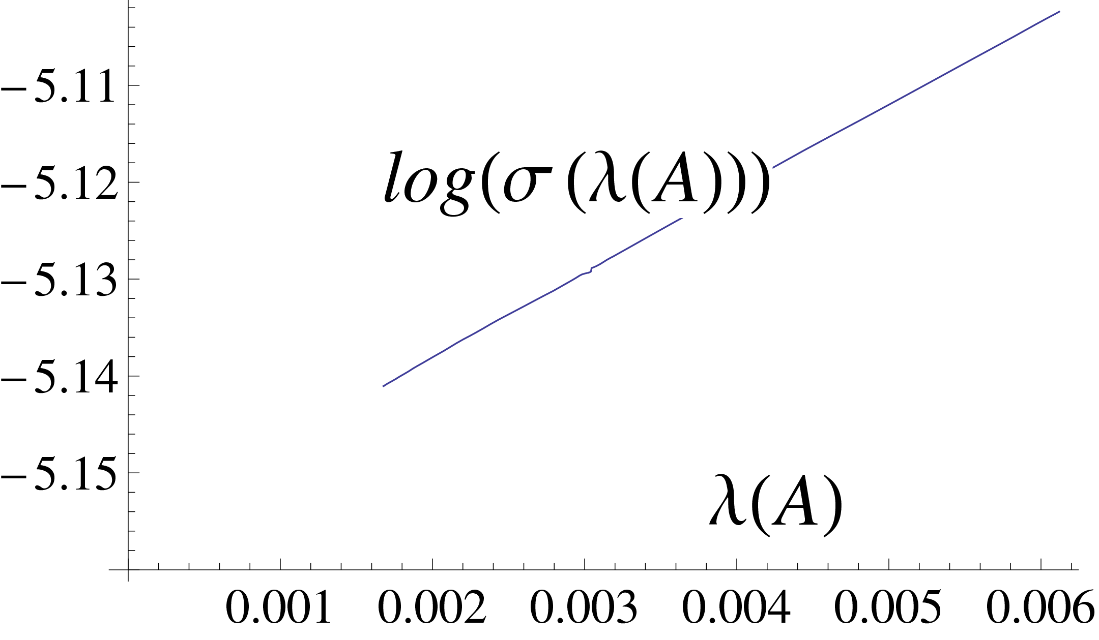
After applying the procedure discussed above, the dominant error in the value of arises actually from the matching of the two tachyon solutions that were obtained by shooting from the UV and from the IR. The solutions are not exactly proportional for due to nonlinearities in the tachyon EoM and coupling to other fields. The error can be reduced by introducing a further subtraction trick that effectively reduces the value of of the solution that was obtained by shooting form the IR, so that the matching can be done for slightly higher values of where the coupling effects are considerably reduced.
We follow [22] and construct two solutions with small but different values . Optimal choice is to take as small as possible and choose one solution with a positive value and another with a negative one. Then we construct
| (E.157) |
where the ratio can be accurately determined as the ratio of the solutions at large (say ).2323 23 There is a small technicality involved in this procedure as the two solutions will in general have different values of . Changing is equivalent with shifts of in -coordinates (see Eq. (E.155)), so we can fix the issue by shifting, say, the solution by a small , obtained by requiring that the corresponding solutions for the coupling match at large . Notice also that the resulting is only useful in the UV region . The point is that the constructed has its several orders of magnitude closer to zero than either of the solutions . Moreover, the residual dependence of on is drastically reduced: the linear corrections cancel in (E.157) (see [22]). The improved value of can now be found by matching with the solution , which was obtained by shooting from the UV, as discussed above.
References
- [1] G. Veneziano, “U(1) Without Instantons,” Nucl. Phys. B 159 (1979) 213.
- [2] T. Banks, A. Zaks, “On the Phase Structure of Vector-Like Gauge Theories with Massless Fermions,” Nucl. Phys. B196 (1982) 189.
- [3]
W. E. Caswell,
“Asymptotic Behavior of Nonabelian Gauge Theories to Two Loop Order,”
Phys. Rev. Lett. 33 (1974) 244;
D. R. T. Jones, “Two Loop Diagrams in Yang-Mills Theory. (Talk),” Nucl. Phys. B 75, 531 (1974). - [4] V.L.Berezinskii, Zh. Eksp.Teor.Fiz. 59, 907 (1970); J.M.Kosterlitz and D.J.Thouless, J. Phys. C6, 1181 (1973).
- [5] V. A. Miransky, “Dynamics of Spontaneous Chiral Symmetry Breaking and Continuum Limit in Quantum Electrodynamics,” Nuovo Cim. A90, 149-170 (1985).
- [6] M. G. Alford, K. Rajagopal, F. Wilczek, “QCD at finite baryon density: Nucleon droplets and color superconductivity,” Phys. Lett. B422 (1998) 247-256 [arXiv:hep-ph/9711395].
- [7] M. G. Alford, K. Rajagopal, F. Wilczek, “Color flavor locking and chiral symmetry breaking in high density QCD,” Nucl. Phys. B537 (1999) 443-458 [arXiv:hep-ph/9804403].
- [8] For a review of recent work, see talks at Lattice2012 by Joel Giedt and Marco Panero.
- [9] M. Teper, “Large N and confining flux tubes as strings - a view from the lattice,” Acta Phys. Polon. B 40, 3249 (2009) [arXiv:0912.3339[hep-lat]].
- [10] Z. Fodor, K. Holland, J. Kuti, D. Nogradi, C. Schroeder, K. Holland, J. Kuti and D. Nogradi et al., “Twelve massless flavors and three colors below the conformal window,” Phys. Lett. B 703, 348 (2011) [arXiv:1104.3124[hep-lat]].
- [11] X. -Y. Jin and R. D. Mawhinney, “Evidence for a First Order, Finite Temperature Phase Transition in 8 Flavor QCD,” PoS LATTICE 2010, 055 (2010) [arXiv:1011.1511[hep-lat]].
- [12] K. Miura, M. P. Lombardo and E. Pallante, “Chiral phase transition at finite temperature and conformal dynamics in large Nf QCD,” Phys. Lett. B 710, 676 (2012) [arXiv:1110.3152[hep-lat]].
- [13] J. B. Kogut and D. K. Sinclair, “Thermodynamics of lattice QCD with 3 flavours of colour-sextet quarks,” Phys. Rev. D 85, 054505 (2012) [arXiv:1111.3353[hep-lat]].
- [14] R. D. Pisarski, “Finite Temperature Qcd At Large N,” Phys. Rev. D 29, 1222 (1984).
- [15] A. Dumitru and R. D. Pisarski, “Degrees of freedom and the deconfining phase transition,” Phys. Lett. B 525, 95 (2002) [arXiv:hep-ph/0106176].
- [16] T. Appelquist, A. Ratnaweera, J. Terning and L. C. R. Wijewardhana, “The Phase structure of an SU(N) gauge theory with N(f) flavors,” Phys. Rev. D 58, 105017 (1998) [arXiv:hep-ph/9806472].
- [17] F. Sannino and J. Schechter, “Chiral phase transition for SU(N) gauge theories via an effective Lagrangian approach,” Phys. Rev. D 60, 056004 (1999) [arXiv:hep-ph/9903359].
- [18] J. T. Lenaghan, D. H. Rischke and J. Schaffner-Bielich, “Chiral symmetry restoration at nonzero temperature in the SU(3)(r) x SU(3)(l) linear sigma model,” Phys. Rev. D 62, 085008 (2000) [arXiv:nucl-th/0004006].
- [19] P. Calabrese and P. Parruccini, “Five loop epsilon expansion for U(n) x U(m) models: Finite temperature phase transition in light QCD,” JHEP 0405, 018 (2004) [arXiv:hep-ph/0403140].
- [20] A. Karch and A. O’Bannon, “Chiral transition of N=4 super Yang-Mills with flavor on a 3-sphere,” Phys. Rev. D 74, 085033 (2006) [arXiv:hep-th/0605120].
- [21] Y. Kikukawa, M. Kohda and J. Yasuda, “First-order restoration of SU(Nf) x SU(Nf) chiral symmetry with large N(f) and Electroweak phase transition,” Phys. Rev. D 77, 015014 (2008) [arXiv:0709.2221 [hep-ph]].
- [22] M. Järvinen and E. Kiritsis, “Holographic Models for QCD in the Veneziano Limit,” JHEP 1203 (2012) 002 [arXiv:1112.1261[hep-ph]].
- [23] R. Narayanan and H. Neuberger, “Chiral symmetry restoration at finite temperature in the planar limit,” Phys. Lett. B 638, 546 (2006) [arXiv:hep-th/0605173].
- [24] L. McLerran and R. D. Pisarski, “Phases of cold, dense quarks at large N(c),” Nucl. Phys. A 796, 83 (2007) [arXiv:0706.2191[hep-ph]].
- [25] T. Kahara and K. Tuominen, “Effective models of two-flavor QCD: Finite and -dependence,” Phys. Rev. D 82, 114026 (2010) [arXiv:1006.3931[hep-ph]].
- [26]
U. Gursoy and E. Kiritsis,
“Exploring improved holographic theories for QCD: Part I,”
JHEP 0802 (2008) 032
[arXiv:0707.1324[hep-th]];
U. Gursoy, E. Kiritsis, F. Nitti, “Exploring improved holographic theories for QCD: Part II,” JHEP 0802, 019 (2008) [arXiv:0707.1349[hep-th]];
E. Kiritsis, “Dissecting the string theory dual of QCD,” Fortsch. Phys. 57 (2009) 396 [arXiv:0901.1772[hep-th]]. - [27] U. Gursoy, E. Kiritsis, L. Mazzanti, F. Nitti, “Deconfinement and Gluon Plasma Dynamics in Improved Holographic QCD,” Phys. Rev. Lett. 101 (2008) 181601 [arXiv:0804.0899[hep-th]]; “Holography and Thermodynamics of 5D Dilaton-gravity,” JHEP 0905, 033 (2009) [arXiv:0812.0792[hep-th]]; “Improved Holographic Yang-Mills at Finite Temperature: Comparison with Data,” Nucl. Phys. B820 (2009) 148-177 [arXiv:0903.2859[hep-th]].
- [28] U. Gursoy, E. Kiritsis, L. Mazzanti, G. Michalogiorgakis and F. Nitti, “Improved Holographic QCD,” Lect. Notes Phys. 828 (2011) 79 [arXiv:1006.5461[hep-th]].
- [29] R. Casero, E. Kiritsis, A. Paredes, “Chiral symmetry breaking as open string tachyon condensation,” Nucl. Phys. B787, 98-134 (2007) [arXiv:hep-th/0702155].
- [30]
I. Iatrakis, E. Kiritsis, A. Paredes,
“An AdS/QCD model from Sen’s tachyon action,”
Phys. Rev. D81 (2010) 115004
[arXiv:1003.2377hep-ph]];
“An AdS/QCD model from tachyon condensation: II,” JHEP 1011, 123 (2010) [arXiv:1010.1364[hep-ph]]. - [31] J. Alanen, K. Kajantie and V. Suur-Uski, “Spatial string tension of finite temperature QCD matter in gauge/gravity duality,” Phys. Rev. D 80, 075017 (2009) [arXiv:0905.2032[hep-ph]]; “A gauge/gravity duality model for gauge theory thermodynamics,” Phys. Rev. D 80, 126008 (2009) [arXiv:0911.2114[hep-ph]].
- [32]
S. S. Gubser and A. Nellore,
“Mimicking the QCD equation of state with a dual black hole,”
[arXiv:0804.0434 [hep-th]];
O. DeWolfe, S. S. Gubser and C. Rosen, “A holographic critical point,” Phys. Rev. D 83 (2011) 086005 [arXiv:1012.1864[hep-th]]. - [33] J. Alanen and K. Kajantie, “Thermodynamics of a field theory with infrared fixed point from gauge/gravity duality,” Phys. Rev. D 81, 046003 (2010) [arXiv:0912.4128[hep-ph]].
- [34]
J. Alanen, K. Kajantie and K. Tuominen,
“Thermodynamics of Quasi Conformal Theories From Gauge/Gravity
Duality,”
Phys. Rev. D 82, 055024 (2010)
[arXiv:1003.5499[hep-ph]];
J. Alanen, T. Alho, K. Kajantie and K. Tuominen, “Mass spectrum and thermodynamics of quasi-conformal gauge theories from gauge/gravity duality,” Phys. Rev. D 84, 086007 (2011) [arXiv:1107.3362[hep-th]]. - [35] C. Nunez, I. Papadimitriou and M. Piai, “Walking Dynamics from String Duals,” Int. J. Mod. Phys. A 25 (2010) 2837 [arXiv:0812.3655[hep-th]].
- [36] S. Prem Kumar, D. Mateos, A. Paredes and M. Piai, “Towards holographic walking from N=4 super Yang-Mills,” JHEP 1105 (2011) 008 [arXiv:1012.4678[hep-th]].
- [37]
L. Anguelova,
“Electroweak Symmetry Breaking from Gauge/Gravity Duality,”
Nucl. Phys. B 843, 429 (2011)
[arXiv:1006.3570[hep-th]];
L. Anguelova, P. Suranyi and L. C. R. Wijewardhana, “Holographic Walking Technicolor from D-branes,” Nucl. Phys. B 852 (2011) 39 [arXiv:1105.4185[hep-th]]; “Scalar Mesons in Holographic Walking Technicolor,” Nucl. Phys. B 862, 671 (2012) [arXiv:1203.1968[hep-th]]. - [38] D. Kutasov, J. Lin and A. Parnachev, “Conformal Phase Transitions at Weak and Strong Coupling,” Nucl. Phys. B 858, 155 (2012) [arXiv:1107.2324[hep-th]].
- [39]
D. K. Hong and H. -U. Yee,
“Holographic estimate of oblique corrections for technicolor,”
Phys. Rev. D 74 (2006) 015011
[arXiv:hep-ph/0602177];
K. Haba, S. Matsuzaki and K. Yamawaki, “S Parameter in the Holographic Walking/Conformal Technicolor,” Prog. Theor. Phys. 120, 691 (2008) [arXiv:0804.3668[hep-ph]];
D. D. Dietrich and C. Kouvaris, “Constraining vectors and axial-vectors in walking technicolour by a holographic principle,” Phys. Rev. D 78, 055005 (2008) [arXiv:0805.1503[hep-ph]]; “Generalised bottom-up holography and walking technicolour,” Phys. Rev. D 79 (2009) 075004 [arXiv:0809.1324[hep-ph]];
D. D. Dietrich, M. Järvinen and C. Kouvaris, “Mixing in the axial sector in bottom-up holography for walking technicolour,” JHEP 1007, 023 (2010) [arXiv:0908.4357[hep-ph]]. - [40] D. Kutasov, J. Lin and A. Parnachev, “Holographic Walking from Tachyon DBI,” Nucl. Phys. B 863, 361 (2012) [arXiv:1201.4123[hep-th]].
- [41] C. Nunez, A. Paredes and A. V. Ramallo, “Unquenched Flavor in the Gauge/Gravity Correspondence,” Adv. High Energy Phys. 2010, 196714 (2010) [arXiv:1002.1088[hep-th]].
- [42]
O. Bergman, S. Seki and J. Sonnenschein,
“Quark mass and condensate in HQCD,”
JHEP 0712, 037 (2007)
[arXiv:0708.2839[hep-th]];
A. Dhar and P. Nag, “Sakai-Sugimoto model, Tachyon Condensation and Chiral symmetry Breaking,” JHEP 0801, 055 (2008) [arXiv:0708.3233[hep-th]];
A. Dhar and P. Nag, “Tachyon condensation and quark mass in modified Sakai-Sugimoto model,” Phys. Rev. D 78, 066021 (2008) [arXiv:0804.4807[hep-th]];
N. Jokela, M. Järvinen and S. Nowling, “Winding effects on brane/anti-brane pairs,” JHEP 0907, 085 (2009) [arXiv:0901.0281[hep-th]]. - [43] D. B. Kaplan, J. -W. Lee, D. T. Son, M. A. Stephanov, “Conformality Lost,” Phys. Rev. D80, 125005 (2009) [arXiv:0905.4752[hep-th]].
- [44]
M. Järvinen and F. Sannino,
“Holographic Conformal Window - A Bottom Up Approach,”
JHEP 1005, 041 (2010)
[arXiv:0911.2462[hep-ph]];
O. Antipin and K. Tuominen, “Constraints on Conformal Windows from Holographic Duals,” Mod. Phys. Lett. A 26, 2227 (2011) [arXiv:0912.0674[hep-ph]];
R. Alvares, N. Evans and K. -Y. Kim, “Holography of the Conformal Window,” Phys. Rev. D 86, 026008 (2012) [arXiv:1204.2474[hep-ph]]. - [45] D. Arean, I. Iatrakis, M. Järvinen, E. Kiritsis, work in progress.
- [46] K. Tuominen, “Finite Temperature Phase Diagrams of Gauge Theories,” [arXiv:1206.5772 [hep-ph]].
- [47] J. Noronha, “Polyakov Loops in Strongly-Coupled Plasmas with Gravity Duals,” J. Phys. G G 37 (2010) 094018 [arXiv:1001.3155[hep-th]].
- [48] M. Panero, “Thermodynamics of the QCD plasma and the large-N limit,” Phys. Rev. Lett. 103 (2009) 232001 [arXiv:0907.3719[hep-lat]].
- [49]
J. Braun and H. Gies,
“Chiral phase boundary of QCD at finite temperature,”
JHEP 0606, 024 (2006)
[arXiv:hep-ph/0602226];
JHEP 1005, 060 (2010)
[arXiv:0912.4168[hep-ph]];
M. Järvinen and F. Sannino, “Extreme Technicolor and The Walking Critical Temperature,” JHEP 1102, 081 (2011) [arXiv:1009.5380[hep-ph]];
J. Braun, C. S. Fischer and H. Gies, “Beyond Miransky Scaling,” Phys. Rev. D 84, 034045 (2011) [arXiv:1012.4279[hep-ph]]. - [50] D.M.Broun, “What lies beneath the dome?,” Nature Physics 4, 170 (2008).
- [51] M. Teper, “Large N,” PoS LATTICE 2008 (2008) 022 [arXiv:0812.0085[hep-lat]].
- [52] K. Kajantie, M. Krssak, M. Vepsalainen and A. Vuorinen, “Frequency and wave number dependence of the shear correlator in strongly coupled hot Yang-Mills theory,” Phys. Rev. D 84, 086004 (2011) [arXiv:1104.5352[hep-ph]].