INTEGRABLE COMBINATORICS
Abstract.
We review various combinatorial problems with underlying classical or quantum integrable structures. (Plenary talk given at the International Congress of Mathematical Physics, Aalborg, Denmark, August 10, 2012.)
Key words and phrases:
integrability, quantum gravity, integrable lattice model, cluster algebra, Laurent phenomenon, tree, alternating sign matrix, plane partition, lattice paths, networks.1. Introduction
In these notes, we present a few mathematical problems or constructs, most of them combinatorial in nature, that either were introduced to explicitly solve or better understand physical questions (Mathematical Physics) or can be better understood in the light of physical interpretations (Physical Mathematics). The frontier between the two is subtle, and we will try to make this more concrete in the examples chosen below.
We start from two different physical theories of discretized random surfaces, describing the possible fluctuations of an underlying two-dimensional discrete space time or equivalently of a discretized Lorentzian[1] (Sect. 2) or Euclidian[38] (Sect. 3) 1+1- or 2-dimensional metric. In both simple models, we show the existence of some hidden integrable structure, in two very different forms. The first model may be equipped with an infinite family of commuting transfer matrices[9] governing the time-evolution of the surfaces, thus displaying quantum integrability, with an infinite number of conserved quantities. The second model actually addresses the correlations of marked points on the discrete surface at prescribed geodesic distance, and we show that such correlations viewed as evolutions in the geodesic distance variable, form a discrete classical integrable system with some conserved quantities modulo the equations of motion[8]. Remarkably, both cases can be reduced bijectively to statistical ensembles of trees.
Few combinatorial objects form such a vivid crossroads between various physical and mathematical theories and constructs as the Alternating Sign Matrices[6]. These were defined by Robbins and Rumsey[35] in an attempt to generalize the notion of determinant of a square matrix, while keeping certain properties, in particular the Laurent polynomiality of the result in terms of the matrix elements. Interestingly, this happened two decades before a combinatorial theory of the Laurent phenomenon was discovered by Fomin and Zelevinsky, under the name of Cluster Algebra[20]. In Sect. 4, we try to unravel the thread from alternating sign matrices to integrable lattice models, back to more combinatorial objects such as plane partitions. We show that the refined enumeration of such objects involves underlying integrable structures similar to that of discrete Lorentzian gravity. This fact is actually used to prove the Mills Robbins Rumsey conjecture[33] relating alternating sign matrices to descending plane partitions. Section 5 is devoted to the cluster algebra formulation and explicit solution of the celebrated T-system[28], a discrete 2+1-dimensional integrable system[27] related to alternating sign matrices, but also to domino tilings of the Aztec diamond[18, 37] and Littlewood-Richardson coefficients[24]. We show that solving such a system amounts to computing partition functions of weighted path models, a kind of discrete path integral, that gives a new insight on the Laurent positivity conjecture of cluster algebra.
2. 1+1D Lorentzian gravity, integrability and trees
2.1. 1+1D Lorentzian gravity
Discrete models for 1+1D Lorentzian gravity are defined as follows. They involve a statistical ensemble of discrete space-times, which may be modeled by random triangulations with a regular time direction (a segment ) and a random space direction, obtained by random triangulations of unit time strips by arbitrary but finite numbers of triangles with one edge along the time line (resp. ) and the opposite vertex on the time line (resp. ). All other edges are then glued to their neighbors so as to form a triangulation. The boundary may be taken free, periodic or staircase-like on the left [9]. A typical such Lorentzian triangulation in 1+1D reads as follows:
These triangulations are best described in the dual picture by considering triangles as vertical half-edges and pairs of triangles that share a time-like (horizontal) edge as vertical edges between two consecutive time-slices. We may now concentrate on the transition between two consecutive time-slices which typically reads as follows:
| (2.1) |
with say half-edges on the bottom and on the top (here for instance we have and ). Denoting by and , the bottom and top states bases, we may describe the generation of a triangulation by the iterated action of a transfer operator with matrix elements . Note that the corresponding matrix is infinite. We shall deal with such matrices in the following. A useful way of thinking of them is via the double generating function:
2.2. Integrability
To make the model more realistic, we may include both area and curvature-dependent terms, by introducing Botlzmann weights equal to the product of local weights of the form per triangle (area term) and per pair of consecutive triangles in a time-slice pointing in the same direction (both up or both down). The rules in the dual picture are as follows:
For instance, in the example (2.1) above with and , the product of local weights is . It is easy to see that these weights correspond to a new transfer operator with matrix elements
Equivalently, the double generating function reads:
| (2.2) |
This model turns out to provide one of the simplest examples of quantum integrable system, with an infinite family of commuting transfer matrices. Indeed, we have:
Theorem 2.1.
[9] The transfer matrices and commute if and only if the parameters are such that where:
This is easily proved by using the generating functions, and noting that for two infinite matrices we have formally , where stands for the convolution product, namely
where the contour integral picks up the constant term in .
2.3. Trees
For suitable choices of boundary conditions, the dual random Lorentzian triangulations introduced above may be viewed as random plane trees. This is easily realized by gluing all the bottom vertices of parallel vertical edges whose both top and bottom halves contribute to the curvature term (no interlacing with the neighboring time slices). A typical such example reads:
Note that the tree is naturally rooted at its bottom vertex.
To summarize, we have unearthed some integrable structure attached naturally to plane trees, one of the most fundamental objects of combinatorics. Note that in tree language the weights are respectively per edge, and per pair of consecutive descendent edges and per pair of consecutive leaves at each vertex (from left to right).
3. Planar maps and geodesics
3.1. Two-dimensional quantum gravity
Two-dimensional quantum gravity (2DQG) is a theory describing the interactions of matter with the underlying space-time, in which both are quantized. Discrete models of 2DQG involve statistical matter models defined on statistical ensembles of discrete random surfaces, in the form of random tessellations. The Einstein action for these 2D random surfaces involves their two invariants, the area and the genus. The complete model will therefore combine the Boltzmann weights of the statistical matter model and of the underlying surface, in the form of parameters coupled to its area and its genus. Matrix integrals have proven to be extremely powerful tools for generating such discrete random surfaces with matter, by noting that the expansion for large matrix size matches the genus expansion. In a parallel way, the field theoretical descriptions of the (critical) continuum limit of 2DQG have blossomed into a more complete picture with identification of relevant operators and computation of their correlation functions. This was finally completed by an understanding in terms of the intersection theory of the moduli space of curves with punctures and fixed genus. Remarkably, in all these approaches a common integrable structure is always present. It takes the form of commuting flows in parameter space.
However, a number of issues were left unadressed by the matrix/field theoretical approaches. What about the intrinsic geometry of the random surfaces? Correlators must be integrated w.r.t. the position of their insertions, leaving us only with topological invariants of the surfaces. But how to keep track say of the geodesic distances between two insertion points, while at the same time summing over all surface fluctuations?
3.2. Maps and trees
Answers to these questions came from a better combinatorial understanding of the structure of the (planar) tessellations involved in the discrete models. And, surprisingly, yet another form of integrability appeared. Following pioneering work of Schaeffer [36], it was observed that all models of discrete 2DQG with a matrix model solution (at least in genus 0) could be expressed as statistical models of (decorated) trees, and moreover, the decorations allowed to keep track of geodesic distances between some faces of the tessellations. Marked planar tessellations of physicists are known as rooted planar maps in mathematics. They correspond to connected graphs (with vertices, edges, faces) embedded into the Riemann sphere. Such maps are usually represented on a plane with a distinguished face “at infinity”, and a marked edge adjacent to that face. The degree of a vertex is the number of distinct half-edges adjacent to it, the degree of a face is the number of edges forming its boundary.
Let us concentrate on the following example of tetravalent (degree 4) planar maps with 2 univalent (degree 1) vertices, one of which is singled out as the root. The Schaeffer bijection associates to each of these a unique rooted tetravalent (with inner vertices of degree 4) tree called blossom-tree, with two types of leaves (black and white), and such that there is exactly one black leaf attached to each inner vertex.
This is obtained by the following cutting algorithm: travel clockwise along the bordering edges of the face at infinity, starting from the root. For each traversed edge, cut it if and only if after the cut, the new graph remains connected, and replace the two newly formed half-edges by a black and a white leaf respectively in clockwise order. Once the loop is traveled, this has created a larger face at infinity. Repeat the procedure until the graph has only one face left: it is the desired blossom-tree, which we reroot at the other univalent vertex, while the original root is transformed into a white leaf.
Why is it a bijection? Remarkably, the information of black and white leaves is sufficient to close up the blossom-tree into a unique map. Clockwise around the tree, match each black leaf to its immediate follower if it is white, and repeat until all but one leaves are matched. The loser of the musical chairs is the root of the map.
3.3. Exact enumeration and integrability
The bijection above allows to keep track of the geodesic distance between the faces containing the two univalent vertices, defined as the minimal number of edges crossed in paths between the two faces (this distance is 2 in the example). Let us introduce a weighted counting of the maps, by including a weight per vertex.
Defining to be the generating function for maps with geodesic distance between the two univalent vertices, we have the following relation:
| (3.1) |
easily derived by inspecting the environment of the vertex attached to the root of the tree when it exists.
This recursion relation must be supplemented with boundary conditions. First, when , the relation (3.1) makes sense only if the term is omitted, so we set . Moreover, if we take , we simply relax the distance condition, and the function is the generating function for maps with two univalent vertices. It satisfies the limiting equation , and we easily get
| (3.2) |
as the unique solution with a formal power series expansion of the form .
The function is the unique solution to (3.1) for such that (i) and (ii) of (3.2). A first remark is in order: the equation (3.1), viewed as governing the evolution of the quantity in the discrete time variable , is a classical discrete integrable system. By this we mean that it has a discrete integral of motion, expressed as follows. The function defined by
| (3.3) |
is such that for any solution of the recursion relation (3.1), the quantity is independent of . In other words, the quantity is conserved modulo (3.1). This is easily shown by factoring .
By the conservation of , we find that
which gives us an explicit relation between and . It turns out that we can solve explicitly for :
Theorem 3.1.
[8] The generating function for rooted tetravalent planar maps with two univalent vertices at geodesic distance at most from each other reads:
where is the unique solution of the equation:
with a power series expansion of the form .
The form of the solution in Theorem 3.1 is that of a discrete soliton with tau-function . Imposing more general boundary conditions on the equation (3.1) leads to elliptic solutions of the same flavor. The solution above and its generalizations to many classes of planar maps have allowed for a better understanding of the critical behavior of surfaces and their intrinsic geometry. Recent developments include planar three-point correlations, as well as higher genus results.
To summarize, we have seen yet another integrable structure emerge in relation to (decorated) trees. This is of a completely different nature from the one discussed in Section 2, where a quantum integrable structure was attached to rooted planar trees. Here we have a discrete classical integrable system, with soliton-like solutions. Such structures will reappear in the following, in relation to (fixed) lattice statistical models.
4. Alternating sign matrices
4.1. Lambda-determinant and Alternating Sign Matrices
The definition of the so-called Lambda-determinant of Robbins and Rumsey [35] is based on the famous Dodgson condensation algorithm [17] for computing determinants, itself based on the Desnanot-Jacobi equation, a particular Plücker relation, relating minors of any square matrix :
| (4.1) |
where stands for the determinant of the matrix obtained from by deleting rows and columns . The relation (4.1) may be used as a recursion relation on the size of the matrix, allowing for efficiently compute its determinant.
More formally, we may recast the algorithm using the so-called -system (also known as discrete Hirota) relation:
| (4.2) |
for any with fixed parity of . Now let be a fixed matrix. Together with the initial data:
| (4.3) |
the solution of the -system (4.2) satisfies:
| (4.4) |
Given a fixed formal parameter , the Lambda-determinant of the matrix , denoted by is simply defined as the solution of the deformed -system
| (4.5) |
subject to the initial condition (4.3).
The discovery of Robbins and Rumsey is that the Lambda-determinant is a homogeneous Laurent polynomial of the matrix entries of degree , and that moreover the monomials in the expression are coded by matrices with entries , characterized by the fact that their row and column sums are and that the partial row and column sums are non-negative, namely
Such matrices are called alternating sign matrices (ASM). These include the permutation matrices (the ASMs with no entry). Here are the 7 ASMs of size 3:
There is an explicit formula for the Lambda-determinant[35]:
| (4.6) |
where and denote respectively the inversion number and the number of entries in , with
Note that for , only the ASMs with contribute, i.e. the permutation matrices, for which coincides with the usual inversion number of the corresponding permutation, and therefore (4.6) reduces to the usual formula for the determinant.
Robbins and Rumsey formulated the famous ASM conjecture, that the total number of ASMs is given by .
4.2. Integrabilities: six vertex, loop gas and more
ASMs relate to two different kinds of integrable systems.
On one hand, the -system relation (4.2) and its deformations (4.5) are known to be discrete classical integrable systems[27], when interpreted as a 2+1D evolution in the discrete time variable . It is also part of a combinatorial structure called a cluster algebra[20], which we will discuss in the next section. As such, it has a guaranteed Laurent property, namely that its solutions are always Laurent polynomials of the initial data, which explains the miracle witnessed by Robbins and Rumsey.
On the other hand ASMs are in bijection with configurations of a famous integrable 2D lattice model, the Six Vertex (6V) model with particular, so-called Domain Wall Boundary Conditions (DWBC) [25, 23]. This latter connection allowed Kuperberg to derive an elegant proof of the ASM conjecture [29], shortly after Zeilberger’s remarkable direct proof using generating functions[39].

The connection with the 6V model is only the tip of an iceberg, which has kept revealing more structure over the years (see the sketch in Fig.1). The ASMs of size are indeed also in same number as:
(i) the Totally Symmetric Self-Complementary Plane Partitions (TSSCPP), namely the rhombus tilings of a regular hexagon of size drawn on the triangular lattice, with all possible symmetries of the hexagon, which amount to the tilings of a fundamental domain occupying of the hexagon (see Fig.1).
(ii) the Descending Plane Partitions (DPP) of order , which we will define below.
There is however no known natural bijection between these objects, and it remains a challenge to find one.
The picture has grown more complex with the remark of Batchelor, DeGier and Nienhuis that the groundstate of the so-called dense loop model on a cylinder of perimeter has positive rational entries summing up to with common denominator . Alternatively, each component is interpreted as the limiting probability of loop configurations realizing a fixed pattern of connection of the string ends on the boundary of the cylinder. Shortly after, the numerator of each component of this vector has been identified by Razumov and Stroganov (RS) as some particular correlation of the 6V model (and equivalently of ASMs), once reformulated as a model of fully-packed loops (FPL) on a square lattice grid [34]. This conjecture was proved recently by Cantini and Sportiello [7] in a purely combinatorial way.
In the next subsections, we will address the connection between refined enumeration of ASMs and DPPs (the Mills, Robbins and Rumsey (MRR) conjecture [33]). Before we go into this, let us mention that more connections have been found between the various combinatorial objects. The computation of the groundstate of the dense loop gas with multi-parameter inhomogeneous Boltzmann weights was performed [14] by use of the so-called quantum Knizhnik-Zamolodchikov equation, whose suitably normalized solution yields the polynomial components of the groundstate vector, depending on complex spectral parameters , and one quantum parameter parameterizing the weight per loop . it was shown [14] that the sum of these components equates the partition function of the 6V model with DWBC when is a non-trivial cubic root of unity, expressed as a determinant by Izergin[23]. The ASM number is recovered in the limit when for all . On the other hand, when all but arbitrary, it was shown that the sum of the components of the groundstate equates the partition function for TSSCPP on the fundamental domain above, with a particular weight for one type of tile [15]. The solutions of the qKZ equation therefore form a bridge between ASM and TSSCPP, in that two different specializations relate to either objects.
Finally, last but not least, yet another combinatorial problem turns out to be related to all of the above. It was shown in [16] that the degree of the variety of strictly upper triangular complex matrices of vanishing square is equal to this weighted TSSCPP counting function, for . Moreover, the variety actually decomposes into irreducible components whose degrees are the entries of the vector, solution to the qKZ equation in the correlated limit where and . More generally this extends to the multi-degree of this variety, by considering its torus-equivariant cohomology, and by taking a suitable limit of the qKZ solution [16, 26].
4.3. ASMs from 6V
The 6V-DWBC model on a square grid has configurations obtained by choosing an orientation for each edge of the square lattice, in such a way that the flow is conserved at each vertex, namely exactly two edges are incoming and two outgoing at each vertex. Moreover the Domain Wall Boundary Conditions impose that horizontal external edges to the grid point into the grid, while vertical ones point out of the grid. This gives rise to the following 6 possible local configurations:
where we also have indicated the corresponding ASM entries. One usually attaches Boltzmann weights to each of the above configurations as follows: each row (resp. column) of the grid carries a complex number , (resp. , ) called spectral parameter. Moreover the weights depend on a “quantum” parameter . We have the following parametrization of the weights:
where is the weight for a vertex of type or at the intersection of a line with parameter and column with parameter , etc. With this parameterization, the model has an infinite family of commuting row-to-row transfer matrices, and can be exactly solved by Bethe Ansatz techniques. Using recursion relations of Korepin[25], Izergin[23] obtained a compact determinantal formula for the partition function of this 6V-DWBC model, defined as the sum over edge configurations of the product of local vertex weights, divided by the normalization factor (to make the answer polynomial in the ’s and ’s). It reads:
| (4.7) |
where stands for the Vandermonde determinant of the ’s.
In the above bijection between 6V configurations and to ASMs, it is easy to track both quantities and in terms of 6V weights. We find that
where , , stand for the total numbers vertex configurations of each type. The determinant result above can therefore be used to compute the refined partition function for ASMs, which counts ASMs with a weight per entry and a weight for each inversion (with these weights, the 7 ASMs of size 3 above have respective weights: ). Setting
| (4.8) |
we have:
| (4.9) |
where refers to the homogeneous limit of the partition function (4.7) of the 6V model in which all are equal to a, etc. (This is obtained by letting all and all , with , and .) This and more refinements were worked out in [3]. We have the following remarkable result:
Theorem 4.1.
[3] The partition function for refined ASM reads:
| (4.10) |
where is any solution to the equation
| (4.11) |
and the determinant is the principal minor for the first rows and columns of the infinite matrix whose entries are generated by
| (4.12) |
We notice that the second term in the generating function is nothing but that of the transfer matrix for 1+1D Lorentzian gravity, up to some gauge transformation and , and upon the identification and .
4.4. DPP from lattice paths
Descending plane partitions are arrays of positive integers of the form:
such that the sequece is strictly decreasing , and that for , :
for all .
The integers are called parts. A DPP is said to be of order if for all . A part is said to be special if . By convention, the empty partition is a DPP. In the following we will compute the partition function which is the sum over all DPP of order with a weight per special part and per remaining part. Here are the 7 DPP of order 3:
They have respective weights: , as the only special part is the entry in the fourth DPP.
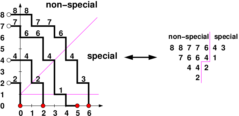
The DPPs are in bijection with configurations of non-intersecting lattice paths illustrated in Fig.2 and defined as follows. We consider the non-negative quadrant of the integer plane. Paths may take two types of step: vertical up or horizontal left. They start along the axis at positions of the form (recorded from right to left) and end along the axis at positions (recorded from top to bottom) for . We add a final horizontal left step at the end of each path. Reading paths from left to right and top to bottom, we record the vertical positions of the -th horizontal step from the left taken on the -th path from top (steps with are not recorded). These form a DPP with rows, of order any . Conversely to each DPP with rows we may associate such a path configuration. Note that the starting points are such that , where the total number of parts in the row . We note that the special parts correspond to horizontal steps taken in the strict upper octant of the plane, and the remaining parts correspond to the horizontal steps in the domain , while horizontal steps along the x axis do not count.
The computation of uses the Lindström-Gessel-Viennot [32, 22] determinant formula expressing the partition function for non-intersecting lattice paths as a determinant where is the partition function for a single path starting from the -th point and ending at the -th. This leads to the following:
Theorem 4.2.
[3] The partition function for DPP of order with weight per special part and per other part reads:
| (4.13) |
where the determinant is the principal minor of size of the infinite matrix with generating function:
| (4.14) |
This bears a striking resemblance to the formula of Theorem 4.1, and also involves the generating function for the transfer matrix of 1+1D Lorentzian gravity.
4.5. Proof of the ASM-DPP conjecture
The complete MRR conjecture is now proved[3]. The proof uses the same ingredients as exposed here, and includes extra refinements. For pedagogical reasons, we retain here only the special/non-special part dependence on the DPP side, and the number of /inversion number dependence on the ASM side. Let us show that:
| (4.15) |
Both expressions are determinants of the principal minor of size of some infinite matrix, in other words, these are the determinants of a finite truncation to the first rows and columns of infinite matrices. There is a very simple relation (independent of ) between the generating functions of the two infinite matrices and , namely:
as a direct consequence of (4.11).
Moreover, introducing the strictly lower triangular infinite “shift” matrix with entries for , we see that for any infinite matrix and any complex parameters : , and similarly . Moreover, as is lower uni-triangular and is upper uni-triangular, any finite truncation to the first rows and columns of and has the same determinant as the corresponding truncation of alone. This allows to identify the principal minors of and and the desired identity follows.
To conclude, our generating function method has allowed for a simple comparison and eventual proof of the identity of the partition functions for ASM and DPP. In passing, it shows some mysterious connection to the quantum integrable transfer matrix of 1+1D Lorentzian gravity. It seems that the quantum integrability of the 6V model is unrelated to this one, and this is yet another puzzling fact about ASMs as a crossroad between various integrable models.
5. Discrete Integrable systems and cluster algebras
5.1. T-system and initial data

Let us concentrate on the T-system realtion (4.5) with for simplicity . We may use this relation to describe the non-linear discrete time evolution () of a 2D space-dependent quantity (for ), , with:
| (5.1) |
Initial conditions determining entirely consist in assigning values of along any fixed “stepped surface” with such that for all . The simplest such surface, denoted by , has mod 2, and consists of all the points at times and (cf. Fig.3). This is the surface used in the definition of the Lambda-determinant. The evolution (5.1) may be used to trade a stepped surface with a surface identical to it except for the point . This is however possible only if the four neighboring points share the same value of . We see that this amounts to completing an octahedron and trading its point with the lowest value of for the one with the largest (see Fig.3). The application of the T-system is sometimes called “octahedron move”.
This will be later interpreted as a mutation at point in the corresponding cluster algebra.
5.2. Cluster Algebra
Here we give a simplified definition of cluster algebra (namely skew-symmetric or geometric type, with no coefficient), and we refer to Fomin and Zelevinsky’s original paper[20] for more general considerations.
Let be an infinite tree with fixed vertex degree , and edges labeled around each vertex. To each vertex of we attach two data: (i) a vector of formal variables with components (ii) an integer skew-symmetric matrix , coding a quiver (graph with oriented edges) with vertices labeled , and with no oriented loops of length .
The data at adjacent vertices of connected via an edge labeled are related via a mutation . The mutation acts both on quivers and data vectors.
The application of on transforms it as follows: (i) it reflects all edges of adjacent to the vertex (ii) for any path of length of the form in , it adds an oriented edge to unless some edges already exist, in which case one of them is canceled. As an example, we represent here the mutations and then on a quiver :
The application of on leaves invariant, except for , where
| (5.2) |
In other words, the quiver at encodes the transformation of the data vector from any adjacent vertex on .
The cluster algebra is the algebra with a unit generated by all the cluster variables at all the clusters. It is entirely determined by the “initial data” at any fixed vertex of the tree . The data vectors are called clusters, their entries cluster variables. The matrix is called exchange matrix. The pair is called a seed. The integer is called the rank of the cluster algebra, and can be infinite.
5.3. Properties, applications, conjectures
The major built-in property of cluster algebras is the Laurent phenomenon: the cluster variables at any vertex of may be expressed as Laurent polynomials of the cluster variables at any other vertex of the tree. This is not obvious, as the mutations involve many divisions. The fact that polynomials are always divisible by the new denominators is a non-trivial outcome of the definitions.
Two important results have been obtained regarding the classification of cluster algebras. First the cluster algebras with finitely many distinct cluster variables (finite type) are classified[21]. In our case, they correspond to an initial quiver that is the Dynkin diagram of a simply-laced Lie algebra of type, with a choice of orientation of the edges. Next, the cluster algebras with finitely many distinct quivers (mutation-finite) are also classified[19]. They are essentially made of cluster algebras attached to (decorated) triangulations of Teichmüller space, plus a few exceptions.
Applications of cluster algebra are very diverse both in mathematics and physics: canonical and dual canonical bases of quantum groups, total positivity, preprojective algebra representations, quiver representations, triangulated 2-Calabi Yau categories, discrete integrable systems and somos-like sequences, dimer models, Donaldson-Thomas invariants of topological string theory, wall-crossing in super-Yang-Mills theories, quantum dilogarithm, Teichmüller space geometry, etc.
A mysterious property was conjectured by Fomin and Zelevinsky[20], and was only proved in particular cases so far: the Laurent phenomenon of cluster algebra is positive, namely the Laurent polynomials involved have only non-negative integer coefficients. This calls for some combinatorial interpretation, still missing to this day.
From now on, we concentrate on the connection to discrete integrable systems, and more precisely to the T-system.
5.4. T-system as a sub-cluster algebra
We have the following:
Theorem 5.1.
[10] The T-system relation is a mutation in an infinite rank cluster algebra.
The initial seed is constructed as follows. The cluster is made of the initial data along the stepped surface discussed above, namely with , and . The quiver may be represented as an infinite square lattice with vertices and oriented edges if mod 2, and otherwise.
Starting from the initial data stepped surface , we may apply a mutation whenever the octahedron move is permitted at (this limits the number of possible mutations, and therefore we do not explore the entire cluster algebra in this way). It is easy to check that in all cases the quiver has 2 incoming and two outgoing edges at each mutable vertex, and the rules (5.2) are equivalent to the T-system relation (5.1). (This can be inferred from the example of mutation given above.).
5.5. Solution and Laurent positivity
Let us briefly describe the solution of the T-system in the case of the initial data surface . The surface can be decomposed into half-octahedra that can be completed upon mutation. We color in white and grey the triangular faces of each half-octahedron as follows, and attach to the “rhombi” formed by pairs of triangles sharing a horizontal edge (belonging to the plane) the following matrices according to whether the grey triangle is on the bottom or the top of the rhombus:
| (5.3) |
where , , and and where the subscript indicates that we should think of these matrices as embedded into an infinite identity matrix with rows and columns indexed by , except at rows and columns where we insert the matrix.
The octahedron move corresponds to the matrix identity
| (5.4) |
which is satisfied iff
By this construction, we represent the T-system mutation by a reordering relation of and matrices.
The solution for and of the T-system with inital data along can be expressed explicitly in terms of the assigned values as the determinant of a matrix built out of products of ’s and ’s. The product is best expressed pictorially:
where the picture is a view from behind of the stepped surface ( from a point with ), the central vertex is and the size of the tilted square is , so that all the boundary vertices sit at time . Moreover, the product is read from left to right, and a D,U is to the left of a D,U in the product iff it is on the picture, with the obvious fact that commute with as soon as . Note that is the embedding of a matrix into an infinite identity matrix. Truncating to the square window we may take its determinant, still denoted .
We have the final:
Theorem 5.2.
[13] The solution of the T-system is expressed in terms of the initial data along the stepped surface as:
This provides an explicitly positive Laurent polynomial of the initial data, due to the structure of the matrices. The proof is by induction under octahedron move, making extensive use of the relation (5.4). This was extended to arbitrary stepped surface initial data[13] as well as other boundary conditions such as wall const. or const. along which is fixed to be . In all cases positivity follows from explicit expressions involving the matrices.
6. Conclusion
In these notes we have explored various combinatorial problems, with one or more links to integrable systems. These links seem to always point to the existence of some kind of tree or path model underlying the original combinatorial problem. Note that a path model is typically a discrete version of a quantum path integral.
In the last section, the solution of the T-system was expressed in terms of matrices. These can be interpreted as elementary pieces allowing to construct networks, namely directed graphs with edge weights. More precisely, we attach to the following elementary pieces of graph, connecting entry and exit vertices labeled via edges oriented from left to right, and whose weights match the corresponding matrix entries:
The above products of matrices correspond to the following networks:
with a total of rows. By the Lindström-Gessel-Viennot theorem, the factor in Theorem 5.2 is the partition function for non-intersecting paths starting at the south-west entry points of the network, and ending at the south-east exit points of the network. This gives yet another path model for the solution of the T-system. The positivity of the path weights is responsible for the positive Laurent phenomenon.
Path models are also very important for non-commutative generalizations. Indeed, a path is a fundamentally non-commuting object, as its steps are taken in a particular order. Attaching non-commuting weights to paths yields natural non-commutative expressions. Cluster algebras have a “quantum” version, in which the cluster variables have commutation relations encoded by the quiver[5]. In rank 2, a fully non-commutative version of cluster algebra was introduced via path model solutions[11, 12]. Finally, a higher rank non-commutative discrete Hirota equation was derived[12] from non-commutative path and continued fraction expressions involving quasi-determinants of non-commuting variables.
References
- [1] J. Ambjorn and R. Loll, Non-perturbative Lorentzian quantum gravity, causality and topology change Nucl. Phys. B 536 (1998) 407–434.
- [2] M.T. Batchelor, J. de Gier and B. Nienhuis, The quantum symmetric XXZ chain at , alternating sign matrices and plane partitions, J. Phys. A 34 (2001) L265–L270. cond-mat/0101385.
- [3] R. Behrend , P. Di Francesco and P. Zinn-Justin , On the weighted enumeration of Alternating Sign Matrices and Descending Plane Partitions. J. Combin. Theory Ser. A 119 (2) (2012), 331–363. arXiv:1103.1176.
- [4] R. Behrend , P. Di Francesco and P. Zinn-Justin , The doubly refined enumeration of Alternating Sign Matrices and Descending Plane Partitions. (2012), arXiv:1202.1520.
- [5] A. Berenstein, A. Zelevinsky, Quantum Cluster Algebras, Adv. Math. 195 (2005) 405–455. arXiv:math/0404446 [math.QA].
- [6] D. Bressoud, Proofs and confirmations: The story of the alternating sign matrix conjecture, MAA Spectrum, Mathematical Association of America, Washington, DC (1999), 274 pages.
- [7] L. Cantini and A. sportiello, Proof of the Razumov-Stroganov conjecture, Journal: J. Comb. Theory A 118 (2011) 1549–1574. arXiv:1003.3376.
- [8] J. Bouttier, P. Di Francesco, and E. Guitter Geodesic distance in planar maps, Nucl. Phys. B 663, No. 3 (2003), 535–567.
- [9] P. Di Francesco, E. Guitter, and C. Kristjansen, Integrable 2D Lorentzian gravity and random walks, Nucl. Phys. B567 No. 3 (2000), 515–553. arXiv:hep-th/9907084.
- [10] P. Di Francesco and R. Kedem, Q-systems as cluster algebras II, Lett. Math. Phys. 89 (2009) 183–216. arXiv:0803.0362 [math.RT].
- [11] P. Di Francesco and R. Kedem, Discrete non-commutative integrability: proof of a conjecture by M. Kontsevich, Int. Math. Res. Notices (2010), doi:10.1093/imrn/rnq024. arXiv:0909.0615 [math-ph].
- [12] P. Di Francesco and R. Kedem, Noncommutative integrability, paths and quasi-determinants, preprint arXiv:1006.4774 [math-ph].
- [13] P. Di Francesco and R. Kedem, T-systems with boundaries from network solutions, preprint arXiv:1208.4333 [math.CO].
- [14] P. Di Francesco and P. Zinn-Justin , Around the Razumov-Stroganov conjecture: proof of a multi-parameter sum rule. Electron. J. Combin. 12 (2005), Research Paper 6, 27 pp. arXiv:math-ph/0410061.
- [15] P. Di Francesco and P. Zinn-Justin , Quantum Knizhnik-Zamolodchikov Equation, Totally Symmetric Self-Complementary Plane Partitions and Alternating Sign Matrices. Theor. Math. Phys. 154 (3) (2008), 331–348. arXiv:math-ph/0703015.
- [16] P. Di Francesco and P. Zinn-Justin , Inhomogeneous model of crossing loops and multidegrees of some algebraic varieties. Comm. Math. Phys. 262 (2) (2006), 459–487. arXiv:math-ph/0412031.
- [17] C. Dodgson, Condensation of determinants, Proceedings of the Royal Soc. of London 15 (1866) 150–155.
- [18] N. Elkies, G. Kuperberg, M. Larsen and J. Propp, Alternating-Sign Matrices and Domino Tilings (Parts I and II) Jour. of Alg. Comb. Vol 1, No 2 (1992), 111-132 and Vol 1, No 3 (1992), 219-234.
- [19] A. Felikson, M. Shapiro and P. Tumarkin, Skew-symmetric cluster algebras of finite mutation type, J. Eur. Math. Soc. 14 (2012), 1135–1180. arXiv:0811.1703 [math.CO].
- [20] S. Fomin and A. Zelevinsky Cluster Algebras I. J. Amer. Math. Soc. 15 (2002), no. 2, 497–529 arXiv:math/0104151 [math.RT].
- [21] S. Fomin, A. Zelevinsky, Cluster algebras II: Finite type classification, Invent. Math. 154 (2003), 63–121. arXiv:math/0208229 .
- [22] I. M. Gessel and X. Viennot, Binomial determinants, paths and hook formulae, Adv. Math. 58 (1985) 300–321.
- [23] A. Izergin, Partition function of the six-vertex model in a finite volume, Sov. Phys. Dokl. 32 (1987) 878–879.
- [24] A. Knutson, T. Tao, and C. Woodward, A positive proof of the Littlewood-Richardson rule using the octahedron recurrence, Electr. J. Combin. 11 (2004) RP 61. arXiv:math/0306274 [math.CO]
- [25] V. Korepin, Calculation of norms of Bethe wave functions, Comm. Math. Phys. 86 (1982) 391–418.
- [26] A. Knutson and P. Zinn-Justin , A scheme related to the Brauer loop model. Adv. Math. 214 (1) (2007), 40–77. arXiv:math.AG/0503224.
- [27] I. Krichever, O.Lipan, P.Wiegmann, and A. Zabrodin, Quantum Integrable Systems and Elliptic Solutions of Classical Discrete Nonlinear Equations, Comm. Math. Phys. 188 (1997) 267-304 arXiv:hep-th/9604080.
- [28] A. Kuniba, A. Nakanishi and J. Suzuki, Functional relations in solvable lattice models. I. Functional relations and representation theory. International J. Modern Phys. A 9 no. 30, pp 5215–5266 (1994). arXiv:hep-th/9310060.
- [29] G. Kuperberg, Another proof of the alternating-sign matrix conjecture, Int. Math. Res. Notices No 3 (1996) 139–150. arXiv:math/9712207.
- [30] P. Lalonde, Lattice paths and the antiautomorphism of the poset of descending plane partitions, Discrete Math. 271 (1Ð3) (2003) 311–319.
- [31] C. Krattenthaler, Descending plane partitions and rhombus tilings of a hexagon with a triangular hole, European J. Combin. 27 (7) (2006) 1138–1146. arXiv:math/0310188.
- [32] B. Lindström, On the vector representations of induced matroids, Bull. London Math. Soc. 5 (1973) 85–90.
- [33] W. H. Mills, D. P. Robbins, and H. Rumsey, Alternating sign matrices and descending plane partitions, J. Combin. Theory Ser. A 34 (1983), 340–359.
- [34] A.V. Razumov and Yu.G. Stroganov, Combinatorial nature of ground state vector of O(1) loop model, Theor. Math. Phys. 138 (2004) 333–337; Teor. Mat. Fiz. 138 (2004) 395–400. arXiv:math.CO/0104216.
- [35] D. P. Robbins and H. Rumsey, Determinants and alternating sign matrices, Adv. Math. 62 (1986), 169–184.
- [36] G. Schaeffer, Bijective census and random generation of Eulerian planar maps, Electronic Journal of Combinatorics, vol. 4 (1997) R20; see also G. Schaeffer, Conjugaison d’arbres et cartes combinatoires aléatoires PhD Thesis, Université Bordeaux I (1998).
- [37] D. Speyer, Perfect matchings and the octahedron recurrence, J. Algebraic Comb. 25 No 3 (2007) 309-348. arXiv:math/0402452 [math.CO].
- [38] V.Kazakov, Bilocal regularization of models of random surfaces, Phys. Lett. B150 (1985) 282–284.
- [39] D. Zeilberger, Proof of the alternating sign matrix conjecture, Elec. J. Comb. 3 (2) (1996), R13.