The Linear Model under Mixed Gaussian Inputs:
Designing the Transfer Matrix
Abstract
Suppose a linear model , where inputs are independent Gaussian mixtures. The problem is to design the transfer matrix so as to minimize the mean square error (MSE) when estimating from . This problem has important applications, but faces at least three hurdles. Firstly, even for a fixed , the minimum MSE (MMSE) has no analytical form. Secondly, the MMSE is generally not convex in . Thirdly, derivatives of the MMSE w.r.t. are hard to obtain. This paper casts the problem as a stochastic program and invokes gradient methods.
The study is motivated by two applications in signal processing. One concerns the choice of error-reducing precoders; the other deals with selection of pilot matrices for channel estimation. In either setting, our numerical results indicate improved estimation accuracy - markedly better than those obtained by optimal design based on standard linear estimators.
Some implications of the non-convexities of the MMSE are noteworthy, yet, to our knowledge, not well known. For example, there are cases in which more pilot power is detrimental for channel estimation. This paper explains why.
Index Terms:
Gaussian Mixtures, minimum mean square error (MMSE), estimationI Problem statement
Consider the following linear system
| (1) |
Here is a vector of observations, and and are mutually independent random vectors with known Gaussian Mixture (GM) distributions:
| (2) | ||||
| (3) |
In this work, we assume that is a transfer matrix that we are at liberty to design, typically under some constraints. Specifically, our objective is to design such that can be estimated from with minimum mean square error (MMSE). The MMSE, for a fixed , is by definition [1]
| MMSE | ||||
| (4) |
Here, denotes the 2-norm, is the joint probability density function (PDF) of ,
| (5) |
is the MMSE estimator, and is the PDF of given . The MMSE in equation (4) depends on both through and . Our objective is to solve the following optimization problem
| (6) |
where denotes a prescribed set of matrices that must belong to. Solving this optimization problem is not straightforward. In particular, three hurdles stand out. Firstly, with (2) and (3) as inputs to (1), the MMSE in (4) has no analytical closed form [2]. Thus, the effect of any matrix , in terms of MMSE, cannot be evaluated exactly. Secondly, the MMSE is not convex in . Thirdly, the first and second order derivatives of the MMSE w.r.t cannot be calculated exactly, and accurate approximations are hard to obtain. For these reasons, and in order to make progress, we cast the problem as a stochastic program and invoke the Robbins-Monro algorithm[3, 4]. Very briefly our approach goes as follows: We draw samples from and and use these to compute stochastic gradients of the MMSE. These feed into an iterative gradient method that involves projection.
The contributions of the paper are several:
- •
As always, for greater accuracy, its preferable to use gradients instead of finite difference approximations. For this reason the paper spells out a formula for exact realization of stochastic gradients. Accordingly, the Robbins-Monro algorithm comes to replace the Kiefer-Wolfowitz procedure.
- •
In the design phase, we exploit the known input statistics and update based on samples of the inputs , instead of output . This yields a closed form stochastic gradient, and we prove that it is unbiased.
- •
Numerical experiments indicate that our method has far better accuracy than methods which proceed via linear estimators. The main reason is that the optimal estimator, used here, is non-linear.
- •
It turns out that the non-convexities of the MMSE may have practical implications that deserve being better known. Specifically, in channel estimation, it can be harmful to increase the power of the pilot signal. This paper offers an explanation.
Clearly, in many practical problems, the quantities in (1) are complex-valued. Throughout this paper, however, they will all be assumed real. For the analysis, this assumption introduces no loss of generality, as the real and imaginary parts of (1) can always be treated separately.
The paper is organized as follows. The next section outlines two applications. It also specifies the Gaussian mixtures and motivates their use. Section III illustrates the problem by means of a simple example. Section IV spells out problem (6) in full detail. Section V reviews how the Robbins-Monro method applies. Numerical results are provided in Section VI. Section VII concludes. A large part of the detailed analysis, concerning stochastic gradients, is deferred to the appendix.
II Background and Motivation
The above described matrix design problem appears in various applications of interest. Next we present two of these, which are of particular interest to the signal processing community. Then we will explain and motivate the GM input statistics.
II-A Linear precoder design
Consider a linear system model
| (7) |
where is a known matrix, and is a precoder matrix to be designed such that the mean square error (MSE) when estimating from becomes as small as possible. The vector is random noise. If and are independent and GM distributed, this is a matrix design problem as described in Section I, where is the design parameter. A typical constraint is to require that cannot exceed a certain average power, i.e. . Together with the nature of , this determines in (6).
A linear model with known transfer matrix and GM distributed inputs is frequently assumed within speech and image processing. In these applications, the signal of interest often exhibits multi modal behavior. That feature can be reasonably explained by assuming an underlying GM distribution. The noise is often modeled as Gaussian, which is a special case of a GM. Conveniently, with (2) and (3) as inputs, the MMSE estimator in (5) has a closed analytical form for any given . Selected works exploiting this include [5, 6, 7, 8, 9]. However, none of these works study MSE reducing precoders. These have the potential to significantly improve the estimation accuracy, and should therefore be of interest.
II-B Pilot signal design
Consider a multiple-input-multiple-output (MIMO) communication model
| (8) |
where is a random channel matrix that we wish to estimate with as small MSE as possible, and is a pilot signal to be designed for that purpose. As before, is random noise. In order to estimate with some confidence, we must transmit as least as many pilot vectors as there are columns in . In addition we must assume that the realization of does not change before all pilots have been transmitted. This assumption typically holds in flat, block-fading MIMO systems[10, 11, 12]. With multiple transmitted pilots, model (8) can be written in matrix form as
| (9) |
If is , then this model can be vectorized into (Thm. 2, Ch. 2, [13])
| (10) |
Here denotes the identity matrix, the operator stacks the columns of a matrix into a column vector, and denotes the Kronecker product. Assuming that the channel () and noise () are independent and GM distributed, this is again a design problem as described in Section I, where the pilot matrix is the design parameter. A natural constraint, is to impose power limitations on the transmitted pilots, i.e. . Together with the structure imposed by the Kronecker product, this then determines in (6).
In (10), one may either assume that is pure background noise, or that represents noise and interference. In the former case a Gaussian distribution may be justifiable, whereas in the latter a GM distribution may be more suitable [14, 15]. As for the channel , a GM distribution can account for multiple fading situations. This can be useful, for example if the source is assumed to transmit from multiple locations. Then, the commonly used Rice distribution is unlikely to accurately capture the channel statistics associated with all transmit locations (especially so in urban areas). In fact, in [16] it has been experimentally observed and reported that different transmit locations are indeed associated with different channel statistics. A GM distributed channel, with multiple modes, has the potential to capture this.
The assumption that a channel realization can originate from several underlying distributions is not novel. For instance, all studies assuming channels governed by a Markov Model make this assumption, see e.g. [17, 18] and the references therein. A GM is a special case of an Hidden Markov model, where subsequent observations are independent, rather than governed by a Markov process. In spite of this, to the best of our knowledge, pilot optimization for estimating channels governed by a GM distribution has not been considered in the literature.
II-C Gaussian Mixture distributions
While aimed at minimizing the MSE, most optimization studies on linear precoders[19, 20] or pilot signals[10, 11, 12] utilize only the first and second moments of the input distributions. Commonly, the underlying motivation is that a linear MMSE (LMMSE) estimator is employed. The LMMSE estimator11 1 Among all estimators which are linear (affine) in the observations, the LMMSE estimator obtains the smallest MSE. only relies on first and second order statistics, which conveniently tends to simplify the associated matrix design problem. In fact, the desired matrix can often be obtained as the solution of a convex optimization problem. It is known, however, that the LMMSE estimator is optimal only for the special case when the random signals and are both Gaussian. For all other cases, the LMMSE estimator is suboptimal.
In practice, purely Gaussian inputs are rare. In general, the input distributions may be asymmetric, heavy tailed and/or multi modal. A type of distribution that can accommodate all of these cases is the Gaussian Mixture (GM) distribution. In fact, a GM can in theory represent any distribution with arbitrary accuracy [21], [22]. Therefore, in this work, we assume that the inputs are GM distributed as in (2) and (3). Notation (2) should be read in the distributional sense, where results from a composite experiment. First, source is activated with probability , . Second, that source generates a Gaussian signal with distribution law . For any realized , however, the underlying index is not observable. The noise emerges in an entirely similar, but independent manner. and are index sets. In theory, it suffices that these sets are countable, but in practice they must be finite. Clearly when and are singletons, one falls back to the familiar case of Gaussian inputs.
The mixture parameters, e.g. , are rarely given a priori. Most often they must be estimated, which is generally a non-trivial task[21, 23]. A common approach is to estimate the GM parameters from training data. The expectation maximization (EM) algorithm is well suited, and much used, for that purpose[1, 24, 25]. Briefly, the algorithm relies on observations drawn from the distribution we wish to parametrize, and some initial estimate of the parameters. The observations are used to update the parameters, iteratively, until convergence to a local maximum of the likelihood function. Because the resulting GM parameters depend on the initial estimates, the algorithm can alternatively be started from multiple initial estimates. This produces multiple sets of GM parameters, and each set can be assigned probabilities based on the training data. Our starting point is that the distributions in (2) and (3) have resulted from such, or similar model fitting.
Model (1) with GM inputs (2) and (3) is quite generic, and we have indicated two signal processing applications where the matrix design problem appears. The solution to that problem is, however, essentially application independent. It should therefore be of interest to a wide audience. To the best of our knowledge, it has not been pursued in the literature.
III An illustrative example
We start by studying a special instance of the matrix design problem, where the MMSE for all can be plotted. In general this is not possible, but the following simple example reveals some fundamental properties of the problem. Assume that we wish to design a precoder, as in (7), where and is restricted to be an orthogonal matrix. Equation (7) then simplifies to , where only rotates . Further, let and be independent and identically GM distributed as
where is a scalar and is the unit vector along the -axis. Assume initially that , which corresponds to no rotation. In this case, Figure 1(a) illustrates the densities of (full circles) and (dashed circles), when seen from above. They are identical and sit on top of each other.
8.5,4)
Now, with a precoder that rotates by , the densities of and will look like in Figure 1(b). The latter configuration is preferable from an estimation viewpoint. This is clear from figure 2, where the MMSE is displayed as a function of all rotation angles between 0 and (with ).
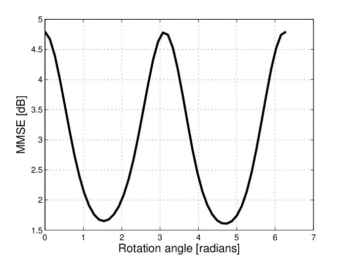
As can be seen, a significant gain can be obtained by rotating (or by ). This gain is not due to a particularly favorable signal-to-noise-ratio ; because is orthogonal, the SNR remains equal for all rotation angles. The MMSE gain is instead due to a rotation producing a signal which tends to be orthogonal to the noise.
The above example is a special case of the matrix design problem, where in (1) is restricted to be orthogonal. It is clear that plays a decisive role in how accurately can be estimated. An almost equally important observation, however, is that the MMSE is not convex in . Hence, in general, we cannot expect that first order optimality (zero gradient) implies a global minimum. When studying the channel estimation problem further, we will see an implication of this non-convexity, which is perhaps not well known: In certain cases the MMSE of the channel estimate does not decrease with increasing pilot power. On the contrary, the MMSE may in fact increase.
In the next section we rewrite the original minimization problem into an equivalent but more compact maximization problem. Then, in Section, V we present a stochastic optimization approach which provides a solution.
IV An equivalent maximization problem
In order to propose a solution to the matrix design problem in (6), we first rewrite expression (4). Using the results of [2], it follows that for model (1), under independent GM inputs (2) and (3), and a fixed , the MMSE can be written as
| (11) |
In (11), denotes the trace operator and is a (GM) probability density function
| (12) |
where
| (13) | ||||
| (14) | ||||
| (15) |
In (13), denotes transposition, denotes the determinant, is short for and is the length of . The MMSE estimator in (11) can be written as
| (16) |
where
| (17) |
In what follows, it is convenient to define
| (18) |
This notation emphasizes that the squared norm of the MMSE estimate depends on both and the observation . In (11), only the integral depends on . Exploiting this, and using (18), the minimizer of the MMSE is that which maximizes
| (19) |
subject to
| (20) |
The integral in (19) cannot be evaluated analytically, even for a fixed and known [2]. Moreover, as the example in Section III illustrated, the MMSE is generally not convex in , which implies that is generally not concave. Hence, any optimization method that merely aims at first order optimality, does in general not produce a global maximizer for . Finally, as argued in the appendix, neither first or second order derivatives of w.r.t. can be computed exactly, and accurate approximations of these are hard to obtain.
V The Robbins-Monro solution
The above observations suggest that a sampling based approach is the only viable option. The problem of maximizing a non-analytical expectation , over a parameter , falls under the umbrella of stochastic optimization. In particular, for our problem, the Robbins-Monro algorithm [3, 4], can be used to move iteratively from a judicially chosen initial matrix to a local maximizer . The philosophy is to update the current matrix using the gradient of the MMSE. Since the gradient cannot be calculated, one instead relies on a stochastic approximation. Translated to our problem, the idea is briefly as follows. Although (19) cannot be computed analytically, it can be estimated from independent sample vectors , as
| (21) |
The derivative of (21) w.r.t. represents an approximation of , which can be used to update the current . Each update is then projected onto the feasible set . This is the core idea of the much celebrated Robbins-Monro algorithm[3]. In our context, the algorithm can be outlined as follows.
- •
Let the current matrix be .
- •
Draw at random and compute .
- •
Calculate the update direction as
(22) and
(23) where is an infinite sequence of step sizes satisfying , and .
- •
Update the matrix as
(24) where represents the projection onto the set of permissible matrices .
- •
Repeat all steps until convergence.
V-A Remarks on the Robbins-Monro algorithm
Recall that the input statistics (2), (3) are assumed known. Therefore, in a design phase, it is reasonable to assume that the inputs can be sampled to compute , as indicated in the second step of the algorithm. The alternative would be to sample directly, leaving the underlying and unknown. The first approach is preferred because it guarantees that (22) becomes an unbiased estimate of , whereas the alternative does not. This important point is fully explained in the appendix. In general, the Robbins-Monro procedure does not require observing the input realizations . The algorithm converges also when only outputs are available. For this reason we write (22) in terms of , but for our implementation we will assume that the underlying inputs are fully known.
Because the gradient direction in (22) is central in the algorithm, its closed form expression is derived in the appendix. Observe that is random because it relies on a random realization of . Specifically it is a stochastic approximation of based on a single observation vector . Instantaneously, it may even point in directions opposite to . In order to increase the likelihood of a beneficial update, one can alternatively compute the gradient as an average based on multiple ’s, as suggested in (21). Then
In our implementation of the algorithm, however, we do not do this. In fact, it was recognized by Robbins and Monro, that choosing large is generally inefficient. The reason is that is only intermediate in the calculations, and as argued in the appendix, regardless of the value of , the update direction can be chosen such that it coincides with in expectation.
The Robbins-Monro procedure does not rely on the existence of at all points. If this derivative is discontinuous, one can instead use any of its sub-gradients; all of which are defined. Consequently, if the local maximum towards which the algorithm converges has a discontinuous derivative, then the algorithm will oscillate around this point. Due to the decaying step sizes, however, the oscillations will eventually become infinitesimal, and for all practical purposes, the system comes to rest.
Convergence towards a local optimum is guaranteed only as [3, 4]. Therefore, in theory, the algorithm must run forever in order to converge. The engineering solution, which tends to work well in practice, is to terminate the algorithm when , where is a chosen threshold, or simply after a predefined number of iterations. Still, the associated running time may be non-negligible, and therefore the Robins-Monro procedure is best suited when the input signals are stationary.
In general, for other problems than considered here, it may happen that the functional form of is unknown, even when its output can be observed for any and . In this case, cannot be computed. Instead one may replace it by a finite difference approximation [26]. In some cases, this may also be preferable even when the derivative can be computed; Especially so if computing requires much effort. When finite difference approximation are used, the procedure is known as the Kiefer-Wolfowitz algorithm [26, 4]. If the derivative can be computed, however, the Kiefer-Wolfowitz algorithm is associated with more uncertainty (larger variance) than the Robbins-Monro procedure. For the interested reader, the present paper extends [27], which considers Kiefer-Wolfowitz precoding.
VI Numerical results
In this section we will study two specific examples. One is on linear precoding, the other is on pilot design for channel estimation. In conformance with much of the literature, we will use the normalized MSE (NMSE) as performance measure22 2 Assuming to be a zero mean signal, the NMSE is never larger than 1 (zero dB). The reason is that the MMSE estimator, , will coincide with the prior mean of only when the SNR tends to zero. Hence, the prior mean is a worst case estimate of , and the NMSE describes the relative gain over the worst case estimate.. This is defined as
VI-A Precoder design
Here we study the performance of a Robbins-Monro precoder. As in the simple example of Section III, we restrict the precoder to be orthogonal. Thus, the norm of precoded signal is equal to that of the non-precoded signal. For the current example we choose the following parameters.
- •
.
- •
is GM distributed with parameters
- •
The noise is Gaussian and distributed as
where is a scalar that can account for any chosen SNR=, and and are the covariance matrices of and respectively.
- •
We use as the initial guess in the Robbins-Monro algorithm.
- •
As stopping criterion we use: .
Because we have assumed , we may in the Robbins-Monro algorithm of Section V simply replace all with the precoder . For the projection in (24), we choose the nearest orthogonal matrix. This projection is the solution to the following optimization problem.
where is the set of orthogonal matrices. The solution is particularly simple, and exploits the singular value decomposition:
Figure 3 displays the NMSE with and without precoding, for increasing SNR levels. As can be seen, Robbins-Monro precoding provides a significant NMSE gain, especially at SNR levels between 0 and 10dB. Observe that the common approach of using the LMMSE estimator (and its corresponding precoder) is highly suboptimal at intermediate SNR levels. In fact, it is much worse than doing MMSE estimation without any precoding.
The above example indicates that our method generates a reasonable precoder, for particular GM input distributions. Admittedly, there exists input statistics for which the gain is much less significant. However, in all simulations we have carried out, the clear tendency is that a Robbins-Monro precoder/ MMSE receiver outperforms the LMMSE precoder/LMMSE receiver at intermediate SNR levels.

VI-B Pilot design for channel estimation
Also for the channel estimation problem, the Robbins-Monro pilot matrix/ MMSE receiver outperforms the LMMSE pilot matrix/LMMSE receiver at intermediate SNR levels. In the next example we choose parameters in order to highlight this, and one additional property. That property is a direct consequence of the non-convex nature of the MMSE. We believe it to be of interest, but not well known. The starting point is the channel estimation problem in (9), where we assume that all matrices are . In the corresponding vectorized model
| (37) |
we assume the following parameters.
- •
The vectorized channel, , is distributed as .
- •
The vectorized noise, , is GM distributed with parameters
(39) - •
As constraint we impose that , where is a positive scalar that can account for any chosen pilot power, and therefore also any SNR=.
- •
Stopping criterion: .
As starting point for the Robbins-Monro algorithm we set equal to a scaled identity matrix satisfying the power constraint. During the iterations we rely on the following simple projection: If the candidate pilot matrix has power , then . Thus, if the pilot matrix does not use the entire power budget, the magnitude of all its elements are increased. Similarly, if pilot matrix has to large power, the magnitude of its elements are decreased.
Figure 4 shows the estimation accuracy for increasing SNR (increasing values of ).

It can bee seen that our method outperforms the commonly used LMMSE channel estimator/LMMSE pilot matrix at intermediate SNRs. In fact, for the same range of SNRs, the latter is much than transmitting a scaled identity pilot matrix and using the MMSE estimator. As the SNR increases, however, it is known that the LMMSE estimator becomes optimal[2]. The performance gap between our approach and the LMMSE estimator at high SNR indicates that a scaled identity pilot matrix is a local optimum that the Robbins-Monro algorithm does not easily escape from. The most striking observation in figure 4, however, is that the channel estimates may become worse by increasing the pilot power! This is not an artifact of the Robbins-Monro algorithm; the same tendency is seen when a scaled identity (satisfying the same power constraint) is used as the pilot matrix.
VI-C Increased pilot power improved channel estimates
We believe that the above phenomenon is not well known, and that it deserves to be explained. In order to visualize what happens, we will consider an example of smaller dimensions, but with similar properties as in the previous subsection. Specifically, we will assume that the unknown channel matrix is , and that the pilot signal is just a scalar, . Then, using (10) it follows that . Thus, in this setup, we do not optimize anything, we only try to explain the NMSE as function of different values for . We assume the following parameters:
- •
, where is a scalar that we can vary.
- •
The signal (channel) is distributed as .
- •
The noise is GM distributed with parameters
(41)
In figure 5, the NMSE is plotted as a function of increasing values for the scalar . We observe the same tendency as in figure 4: for increasing values of (corresponding to increasing pilot power in figure 4), the NMSE may increase. In figure 5, we also plot the NMSE that would be obtained by a genie aided estimator [2]. Briefly, the genie aided estimator knows from which underlying Gaussian source the noise originates for each observation . Accordingly it can always produce the MMSE estimate corresponding to a purely Gaussian model. The genie aided estimator can of course not be implemented in practice, but because it is much better informed than the MMSE estimator, it provides a lower bound on the NMSE. Yet, from figure 5 we see that for dB, the MMSE estimator is able to pin-point the correct noise component.


A plausible explanation is the following. For small , almost all realizations of are close to the origin. Thus, observations tend to appear in two distinct clusters; one cluster centered at each noise component. As a consequence, the active noise component can essentially always be identified. As grows, take values in an increasingly larger area, and the cluster borders approach each other. The value dB is the largest value for where the clusters can still be ’perfectly’ separated. This value corresponds to the local minimum in figure 5. Because we are considering 2-dimensional random vectors, we can actually visualize these clusters. The upper part of figure 6 shows how 400 independent ’s form two nearby, but separable, clusters generated at dB. When grows beyond this level, the receiver faces a larger identification problem: it is harder to tell which noise component was active. The lower part of figure 6 shows 400 independent ’s generated at dB. This value corresponds to the local maximum in figure 5. Here the clusters largely overlap. As continues to grow, however, the average magnitude of a noise contribution becomes so small compared to the average magnitude of , that near perfect recovery of eventually becomes possible.
Translated to the channel estimation problem in figure 4, the interpretation is that there is a continuous range where increasing the pilot power is harmful. From figure 4, one observes that, unless one can spend an additional 15 dB (approximately) on pilot power, one will not improve from the local minimum solution.
VII Conclusion
We have provided a framework for solving the matrix design problem of the linear model under Gaussian mixture statistics. The study is motivated by two applications in signal processing. One concerns the choice of error-reducing precoders; the other deals with selection of pilot matrices for channel estimation. In either setting we use the Robbins-Monro procedure to arrive at a solution. Our numerical results indicate improved estimation accuracy at intermediate SNR levels; markedly better than those obtained by optimal design based on the LMMSE estimator.
Although the Robbins-Monro algorithm in theory only converges asymptotically, in practice we see that a hard stopping criterion may work well. The algorithm is still computationally demanding, and therefore best suited under stationary or near stationary settings.
We have explored an interesting implication of the non-convexity of the MMSE; namely a case where spending more pilot power gives worse channel estimates. This phenomenon is not linked to the stochastic optimization procedure. It can be observed without optimizing at all, and we have offered a plausible explanation.
VIII Acknowledgments
John T. Flåm is supported by the Research Council of Norway under the NORDITE/VERDIKT program, Project CROPS2 (Grant 181530/S10).
This appendix derives a closed form expression for the gradient direction in (22), where is defined through (16)-(18). To that end, it is worth observing that when optimizing it is beneficial if the designer can draw samples directly from the inputs and , and not only the output . In order to see why, assume in what follows that the order of derivation and integration can be interchanged such that
| (42) |
Now, if we can only observe outputs , we have
Hence, in this case, the update direction is not an unbiased estimator of the gradient . In contrast, assume that we can draw inputs , and define
then
Here, the second equality holds because is independent of . Hence, is an unbiased estimator of , which is of course desirable. Because it is beneficial to sample and , rather than just , we will assume here that the designer can do this. In practice, this implies that the optimization of is done off line, as preparation for the subsequent estimation.
In what follows, we will prove that interchanging the order of integration and derivation, as in (42) is justifiable. We will derive a closed form expression for , and use this as the update direction in (22). Our strategy, however, will be to do this in the reverse order: First we compute the derivative, assuming that the change can be done, and then we show that that differentiation under the integral sign is justified. Although we assume knowledge of for each observed , we will write instead of , and instead of , simply to save space.
Using (16), can be written as
| (43) |
In order to compute (43), we make use of the following theorem [13].
Theorem 1
For a scalar function, , of a matrix argument, the differential has the form
In our case, we take to be the expression in the large parenthesis of (43). We will identify its differential, and exploit Theorem 1 in order to obtain the derivative. For that purpose, it is convenient to define
| (44) | ||||
| (45) | ||||
| (46) |
Using these, the derivative in (43), can then be compactly written as . Using the chain rule, the differential of this fraction is
| (47) |
Thus, we must identify the differentials and , which we do in next. Notation: we will in the remainder of this appendix use to compactly denote the trace operator.
Computing
| (48) |
The differential , is a differential of a Gaussian probability density function. In our case it depends on the indexes , but in order to enhance readability, we will disregard these indexes in what follows. Thus, for now, we will use equations (12)-(17) with all indexes removed, and reincorporate the indexes when needed. In addition, we will for now disregard the constant factor in (13). Hence, instead of considering the differential , we therefore consider , where . This can be written as
| (49) |
In the second equality we have used the chain rule, and exploited that is an exponential function. The first differential in (49), provided is full rank, is (Theorem 1, ch. 8, of [13])
| (50) | ||||
| (51) | ||||
| (52) | ||||
| (53) | ||||
| (54) |
In (52), we have rotated the first trace (done a cyclic permutation of the matrix product), and transposed the second trace. Because and are symmetric, they are not affected by transposition. Moreover, . The trace operator is invariant to such rotations and transposition, and therefore these operations are justified. In (53) we have rotated the second term. Such rotations and transpositions will be frequently employed throughout. Introducing , the second differential of (49) can be written
| (55) |
The first term of (55) is
| (56) | ||||
| (57) | ||||
| (58) |
Equation (57) results from Theorem 3, ch. 8, of [13]. Observe that in (58) is a symmetric matrix, playing the same role as in (51). Therefore, we can utilize (54) and conclude that
| (59) |
Recall that . The second term of (55) can therefore be written as
| (60) |
Using (54),(59) and (60), and inserting into (49), we find that
| (61) |
If we define
where , and reincorporate the constant factor , we now find that
| (62) |
Accordingly, (48) becomes
| (63) |
Computing
| (64) |
Apart from a rearrangement of the indexes, equation (64) contains two similar terms. Hence it suffices to compute one of them. Recalling that is defined by (17), we focus on the differential
| (65) | ||||
| (66) | ||||
| (67) |
We will resolve this term by term. The first term, (65), reads
| (68) |
The second term, (66), can be written as
| (69) |
The third term, (67), reads
| (70) |
Using (68),(69) and (70) we now define
Due to its two similar terms, the differential in (64) can then be written
| (71) |
Computing
| (72) |
The last equation results immediately by employing (62).
-A Computing the derivative
Utilizing (63), (71) and (72), the complete differential in (47) can now be written as
| (73) |
In case of a precoder design problem, one makes the following substitutions: and throughout. In case of the pilot design problem (10), must be substituted by . In addition, assuming that is , one makes use of the fact that
Here is the Magnus and Neudecker commutation matrix [13]. Theorem 1 can then be easily applied to (73), and identifying the derivative in (43) is therefore now straightforward.
-B Interchanging the order of derivation and integration
Recall, that interchanging the order of derivation and integration, as in (42), was until now only assumed valid. It derives from Lebesgue’s Dominated Convergence Theorem that such a change is valid if there exists a dominating function satisfying
| (75) |
and
| (76) |
Now consider (74) and define the function
Observe that
Hence is a convex combination of the ’s, and therefore the function
clearly satisfies (75). We do not explcitly prove it her, but it can be verified that the integral
| (77) |
is bounded. Hence a dominating function exists, and the change of integration and derivation is justified.
-C First and second order derivatives of the objective function
When trying to compute
| (78) |
the mixture densities in the denominators of (74) will not simplify by substitutions. An entirely similar argument provides the reason for why (19) cannot be computed analytically in the first place [2]. Hence, (78) cannot be computed analytically, and a closed form derivative of (19) w.r.t does not exist. Although not demonstrated here, a similar argument will hold also for the second order derivative.
References
- [1] Steven M. Kay, Fundamentals of Statistical Signal Processing: Estimation Theory, Prentice-Hall, Inc., Upper Saddle River, NJ, USA, 1993.
- [2] John Flåm, Saikat Chatterjee, Kimmo Kansanen, and Torbjörn Ekman, “On MMSE Estimation - A Linear Model under Gaussian Mixture Statistics,” IEEE Transactions on Signal Processing, 2012.
- [3] Herbert Robbins and Sutton Monro, “A stochastic approximation method,” The Annals of Mathematical Statistics, vol. 22, no. 3, pp. pp. 400–407, 1951.
- [4] H.J. Kushner and G. Yin, Stochastic Approximation and Recursive Algorithms and Applications, vol. 35, Springer Verlag, 2003.
- [5] D. Persson and T. Eriksson, “Mixture Model- and Least Squares-Based Packet Video Error Concealment,” Image Processing, IEEE Transactions on, vol. 18, no. 5, pp. 1048 –1054, may 2009.
- [6] A. Kundu, S. Chatterjee, and T.V. Sreenivas, “Subspace Based Speech Enhancement Using Gaussian Mixture Model,” in Interspeech 2008, Brisbane, Australia, september 2008, pp. 395 –398.
- [7] A. Kundu, S. Chatterjee, and T.V. Sreenivas, “Speech Enhancement using Intra-Frame Dependency in DCT Domain,” in 16th European Signal Processing Conference (EUSIPCO 2008), Lausanne, Switzerland, August 25-29 2008.
- [8] A.D. Subramaniam, W.R. Gardner, and B.D. Rao, “Low-Complexity Source Coding Using Gaussian Mixture Models, Lattice Vector Quantization, and Recursive Coding with Application to Speech Spectrum Quantization,” Audio, Speech, and Language Processing, IEEE Transactions on, vol. 14, no. 2, pp. 524 – 532, march 2006.
- [9] G. Yu, G. Sapiro, and S. Mallat, “Solving Inverse Problems With Piecewise Linear Estimators: From Gaussian Mixture Models to Structured Sparsity,” Image Processing, IEEE Transactions on, vol. PP, no. 99, pp. 1, 2011.
- [10] D. Katselis, E. Kofidis, and S. Theodoridis, “On training optimization for estimation of correlated mimo channels in the presence of multiuser interference,” Signal Processing, IEEE Transactions on, vol. 56, no. 10, pp. 4892 –4904, oct. 2008.
- [11] M. Biguesh and A.B. Gershman, “Training-based mimo channel estimation: a study of estimator tradeoffs and optimal training signals,” Signal Processing, IEEE Transactions on, vol. 54, no. 3, pp. 884 – 893, march 2006.
- [12] E. Bjornson and B. Ottersten, “A framework for training-based estimation in arbitrarily correlated rician mimo channels with rician disturbance,” Signal Processing, IEEE Transactions on, vol. 58, no. 3, pp. 1807 –1820, march 2010.
- [13] Jan R. Magnus and Heinz Neudecker, Matrix Differential Calculus with Applications in Statistics and Econometrics, John Wiley & Sons, 2nd edition, 1999.
- [14] V. Cellini and G. Dona, “A novel joint channel and multi-user interference statistics estimator for uwb-ir based on gaussian mixture model,” in Ultra-Wideband, 2005. ICU 2005. 2005 IEEE International Conference on, sept. 2005, pp. 655 – 660.
- [15] G.E. Healey and R. Kondepudy, “Radiometric CCD Camera Calibration and Noise Estimation,” Pattern Analysis and Machine Intelligence, IEEE Transactions on, vol. 16, no. 3, pp. 267 –276, mar 1994.
- [16] J. Medbo, H. Asplund, J.E. Berg, and N. Jaldén, “Directional Channel Characteristics in Elevation and Azimuth at an Urban Macrocell Base Station,” in 6th European Conference on Antennas and Propagation, March 2012.
- [17] Hong Shen Wang and N. Moayeri, “Finite-state markov channel-a useful model for radio communication channels,” Vehicular Technology, IEEE Transactions on, vol. 44, no. 1, pp. 163 –171, feb 1995.
- [18] P. Sadeghi, R. Kennedy, P. Rapajic, and R. Shams, “Finite-state markov modeling of fading channels - a survey of principles and applications,” Signal Processing Magazine, IEEE, vol. 25, no. 5, pp. 57 –80, september 2008.
- [19] A. Scaglione, P. Stoica, S. Barbarossa, G.B. Giannakis, and H. Sampath, “Optimal Designs for Space-Time Linear Precoders and Decoders,” Signal Processing, IEEE Transactions on, vol. 50, no. 5, pp. 1051 –1064, may 2002.
- [20] D.H. Pham, H.D. Tuan, B.-N. Vo, and T.Q. Nguyen, “Jointly optimal precoding/postcoding for colored mimo systems,” in Acoustics, Speech and Signal Processing, 2006. ICASSP 2006 Proceedings. 2006 IEEE International Conference on, may 2006, vol. 4, p. IV.
- [21] Jonathan Q. Li and Andrew R. Barron, “Mixture Density Estimation,” in In Advances in Neural Information Processing Systems 12. 1999, pp. 279–285, MIT Press.
- [22] H.W. Sorenson and D.L. Alspach, “Recursive Bayesian Estimation Using Gaussian Sums,” Automatica, vol. 7, no. 4, pp. 465 – 479, 1971.
- [23] S. Dasgupta, “Learning Mixtures of Gaussians,” in Foundations of Computer Science, 1999. 40th Annual Symposium on, 1999, pp. 634 –644.
- [24] Zoubin Ghahramani, “Solving Inverse Problems using an EM approach to Density Estimation,” in Proceedings of the 1993 Connectionist Models Summer School, 1993, pp. 316–323.
- [25] David J.C. MacKay, Information Theory, Inference, and Learning Algorithms, Cambridge University Press, 2003.
- [26] J. Kiefer and J. Wolfowitz, “Stochastic Estimation of the Maximum of a Regression Function,” The Annals of Mathematical Statistics, vol. 23, no. 3, pp. pp. 462–466, September 1952.
- [27] J.T. Flåm, M. Vehkaperä, D. Zachariah, and E. Tsakonas, “Mean Square Error Reduction by Precoding of Mixed Gaussian Input,” in International Symposium on Information Theory and its Applications, ISITA 2012, Honolulu - Hawaii, Oct 28- Nov 01, 2012.