Compton scattering from the proton in an effective field theory with explicit Delta degrees of freedom
Abstract
We analyse the proton Compton-scattering differential cross section for photon energies up to using Chiral Effective Field Theory (EFT) and extract new values for the electric and magnetic polarisabilities of the proton. Our approach builds in the key physics in two different regimes: photon energies (“low energy”), and the higher energies where the resonance plays a key role. The Compton amplitude is complete at N4LO, , in the low-energy region, and at NLO, , in the resonance region. Throughout, the Delta-pole graphs are dressed with loops and vertex corrections. A statistically consistent database of proton Compton experiments is used to constrain the free parameters in our amplitude: the transition strength (which is fixed in the resonance region) and the polarisabilities and (which are fixed from data below ). In order to obtain a reasonable fit, we find it necessary to add the spin polarisability as a free parameter, even though it is, strictly speaking, predicted in EFT at the order to which we work. We show that the fit is consistent with the Baldin sum rule, and then use that sum rule to constrain . In this way we obtain and , with for degrees of freedom. A detailed rationale for the theoretical uncertainties assigned to this result is provided.
I Introduction
Compton scattering from the proton, , at photon energies up to a few hundred MeV, has proven an excellent tool to study the subtle interplay of the effective low-energy degrees of freedom of hadrons, and of the symmetries and dynamics which govern them; see recent reviews for details [2, 3, 1]. It reveals the chiral symmetry of QCD and the pattern of its breaking by probing pion-cloud effects, and the properties of the as the lowest nucleonic excitation. Since it tests the (real and virtual) excitation spectrum of the target, probing the two-photon response of a proton also complements the information available in the one-photon response (e.g. form factors).
Since the earliest experiments on the proton [4, 5, 6, 7, 11, 12, 13, 14, 8, 9, 10, 15], a particular goal has been an extraction of the electric and magnetic polarisabilities, and , which parametrise the stiffness of the proton against deformation in uniform, static electric and magnetic fields. At photon energies below 50 MeV the Compton cross section is completely dominated by the Born terms, with the Thomson cross section as the low-energy limit. The polarisabilities manifest themselves as corrections to this point-like cross section which grow as , but there is only a narrow range of energy before faster-varying terms contribute significantly. At MeV non-analytic structure associated with pion photoproduction appears, and around the same energy the tail of the Delta resonance also becomes apparent. In order to extract the polarisabilities, therefore, we need a reliable description of these effects. In this paper we analyse Compton-scattering data in such a framework in order to extract and in a model-independent way. Our tool is Chiral Effective Field Theory, EFT, the low-energy version of QCD [16, 17, 18, 19, 20, 21, 22, 23, 24, 25]. In it, theoretical uncertainties can be estimated using its power counting, namely a systematic expansion scheme for physical observables. As the baryonic sector of Chiral Perturbation Theory (PT) including nucleons and the , it orders all interactions consistent with the symmetries of QCD (and in particular the pattern of its chiral-symmetry breaking) by an expansion in powers of “low” momentum scales in units of a “high” scale at which new degrees of freedom become relevant. Calculating both tree and loop diagrams to a given order in this small parameter results in an amplitude that is truncated at a certain, prescribed level of accuracy.
Indeed, Compton scattering provided one of the early successes of EFT applied to nucleons. Bernard et al. [27, 26] calculated the polarisabilities at leading one-loop order, without explicit degrees of freedom, to be
| (1) |
in remarkably good agreement with both the extractions of these parameters extant at that time, and those obtained in subsequent experiments. Furthermore the cross sections obtained from that theory were in qualitative agreement with the then-available data below about [21, 28]. Subsequently, a large number of experiments [29, 30, 31, 32, 34, 35, 36, 37, 40, 33, 38, 39] have measured unpolarised differential cross sections at photon energies between about 60 and 400 MeV; see the thorough discussions in the reviews [2, 3, 1]. However, we shall argue in this article that the database remains quite sparse in important regions, in particular between 150 and 250 MeV. In addition, there are unresolved consistency issues between data sets from different experiments. Therefore, plans to measure Compton cross sections at MAMI and HIS [41, 42, 43] are very welcome.
Results obtained for and using EFT may be compared to direct determinations from fully dynamical lattice QCD which appear imminent [44, 45, 46, 48, 47]. Such simulations, in turn, take advantage of the fact that EFT reliably predicts the strong dependence of the polarisabilities on the pion mass, so that results can be extrapolated from unphysical quark masses. Thus, Compton scattering provides an excellent example of how EFT serves as a bridge between cross sections measured in experiments and the non-perturbative quark-gluon dynamics underlying the physics of hadrons.
Apart from its relevance in Compton scattering, the magnetic polarisability also contributes the largest error on the two-photon-exchange contribution to the Lamb shift in muonic hydrogen [49, 50, 51]. And, while we focus here on the case of the proton, this study also provides input to extractions of neutron polarisabilities from data on elastic Compton scattering on deuterium; see e.g. Refs [52, 1]. Small proton-neutron differences stem from chiral-symmetry-breaking pion-nucleon interactions, probing details of QCD. For example, Walker-Loud et al. [53] recently found that the biggest uncertainty in theoretical determinations of the electromagnetic proton-neutron mass difference now comes from the contribution of ] MeV from this effect [1]. However, such effects can be probed with confidence only if both experimental and theoretical uncertainties are well under control.
As already mentioned, there has been a significant increase in the data available on scattering over the last twenty years. Over the same period the EFT description of this process has been refined in several ways. The pion-nucleon-loop amplitudes are now known to one order higher [54, 55, 56], where two short-distance contributions to and enter the Compton amplitude. The polarisabilities are then no longer predicted, but can be determined from low-energy Compton data, and the fit quality indicates the extent to which EFT correctly captures the energy-dependence of the Compton amplitudes. This has been done in Refs. [57, 58]. In another line of attack, the was included as an explicit degree of freedom, applying Lagrangians developed in Refs. [59, 61, 60, 62]. This allows for a description which applies from zero photon energy into the Delta resonance region, and thus also for using data at intermediate energies for alternative extractions of the polarisabilities [63, 62]. In both these variants, baryons have traditionally been included as non-relativistic degrees of freedom in a version called “Heavy-Baryon Chiral Perturbation Theory” (HBPT) [19, 20, 26]. A good qualitative reproduction of Compton data in this regime has also been obtained in a EFT calculation which does not invoke the heavy-baryon expansion [64, 65, 66, 67], and the agreement between the cross sections with and without the heavy-baryon expansion is very good—even at leading one-loop order—once the polarisabilities are fixed [68]. In line with the power-counting philosophy, it is encouraging that the extractions or predictions of and have not varied dramatically from the original predictions, as demonstrated by the values advocated in a recent review [1].
In this paper, we merge these three refinements: higher orders in the chiral sector, explicit Delta degrees of freedom, and partially-covariant formulations. In EFT one identifies two low-energy scales, and . Different power countings involving choices about their relative sizes are possible. We follow Pascalutsa and Phillips [63] and use the ratio of the two scales, , as our small parameter. In Compton scattering this has the advantage that it allows us to differentiate between the kinematic regime where and that where . We obtain an amplitude which at low energies is complete at , where the leading (Thomson) amplitude is , while around the Delta resonance the amplitude is complete at order relative to leading order.
We determine and by fitting to the proton Compton-scattering database established in Ref. [1]. To that end, we constrain the parameters of the M1 coupling by the data around the Delta-resonance, and then extract polarisabilities from the data at lower energy. We find that an excellent fit can be obtained by including one contact operator which corresponds to a short-distance contribution to the spin-polarisability —even though, strictly speaking, this effect only appears at one order beyond that to which our calculation is complete. In doing this we are departing from the strict EFT expansion, but the same strategy is necessary at lower order where, once the Delta is included, and must be promoted [62].
This article is structured as follows. First, we define the theoretical ingredients of our calculation: the framework in Sec. II.1; the power counting in the different kinematic regimes and how to arrive at an amplitude which is valid across regimes in Sec. II.2; explicit results for the vertex corrections in Sec. II.3; the prescription for the kinematically-correct position of the pion-production threshold in Sec. II.4; and constraints from sum rules and other processes in Sec. II.5. Sec. III is devoted to the fit itself. We present our results in Sec. III.2, followed by a discussion of details, alternative scenarios and convergence issues as well as, importantly, an estimate of the residual theoretical uncertainties in Sec. III.3. After the Summary and Outlook of Sec. IV, an Appendix gives references for the explicit forms of the components of the amplitudes. Preliminary versions of our findings appeared in Refs. [69, 70, 1].
II Theoretical Ingredients
II.1 Framework
The standard decomposition of the Compton-scattering amplitude is given in Refs. [56, 1], as are the expression relating to the differential cross sections in the centre-of-mass (cm) and laboratory (lab) frames. For our calculations we use the Breit frame in which the photon does not transfer energy to the proton. See Refs. [71, 1] for details of kinematics in the various frames.
As detailed in Ref [1], the Compton amplitude can be split into Born and structure terms, the former arising (in a covariant framework) from nucleon- and pion-pole graphs, and the latter from all other effects. A low-energy expansion of the structure amplitude can be used to define the electric and magnetic scalar polarisabilities and , as well as the four spin polarisabilities. In the Breit frame, such an -expansion gives, for the polarisability contributions to the structure amplitude,
| (2) |
where and ( and ) are the three-momentum and polarisation vector of the incoming (outgoing) photon, and () unit vectors pointing in the direction of ().
The polarisabilities used in Eq. (2) can be generalised to define dynamical, i.e. energy-dependent, polarisabilities [72, 62]. (These should not be confused with the generalised polarisabilities that can be accessed in virtual Compton scattering.) This is equivalent to a multipole decomposition of the structure (i.e. non-Born) part of the Compton amplitude. For further discussion of the definition and usefulness of energy-dependent/dynamical polarisabilities, see Ref. [1]. Here, however, we work with the full amplitudes rather than a truncated multipole decomposition.
We calculate the amplitudes within the framework of EFT. Since the heavy-baryon Lagrangian is well-established, see e.g. Refs. [21, 25]; we do not reproduce it here. We use terms up to fourth order in , using the conventions of Refs. [21, 73, 74]. The terms relevant to Compton scattering at the order to which we work are given in Ref. [1]. Only the leading terms of are required, except for the anomalous part of which governs .
One set of terms though are worth including, since we will refer to them again. At , divergent loops need to be renormalised by operators that occur in . Those relevant for Compton scattering are:
| (3) |
They translate into additional, energy-independent contributions, and , to the electric and magnetic polarisabilities which are isoscalar or isovector.
For the resonance, our calculation uses two variants. As we discuss in Secs. II.2.2 and II.3, we perform a fully Lorentz-covariant calculation of the Delta-pole diagrams. and are taken from Pascalutsa and Phillips [63]. However for loops we use corresponding terms from the heavy-baryon reduction of Hemmert et al. [59] which are reproduced in Ref. [1]. The coupling constant in the latter is denoted , which corresponds to in the former (but see later for a discussion of the appropriate values to use in the two cases).
Because we will refer repeatedly to the couplings, though, we reproduce the relevant terms here. Since we work to NLO in the domain where the photon energy and the Delta-nucleon mass splitting are comparable, , we need selected terms from the Lagrangian up to third order [75]:
| (4) | ||||
| (5) |
where the field of mass is an iso-quadruplet heavy-baryon reduction of the Rarita-Schwinger field [60], () being the index of the isovector (vector) coupled to the isospinor (spinor). is the electron charge. All other symbols have their standard meaning. Terms generated by the heavy-baryon reduction are omitted in Eq. (5). The convention used here is in accord with that of Refs. [76, 77, 62, 1]. In Eq. (5) we have identified Ref. [75]’s .
The interaction is of order , while both the and terms give rise to couplings which are of order .
The corresponding form in the covariant version is [63]:
| (6) |
where , , , and . The (leading) terms involving the electromagnetic field that emerge upon heavy-baryon reduction of this Lagrangian are equivalent to those in Eqs. (4) and (5), provided we make the identification
| (7) |
In this presentation, we use the relativistic variant of the couplings, but quote results in terms of and , using this conversion formula throughout, since these are more widely used. The - and -channel Delta-pole diagrams then reproduce the results given in the Appendices of Ref. [63]. However, the Lagrangians of Refs. [63, 78] do not include a structure that reduces to that with coefficient in Eq. (5); this point will play a role in Sec. II.3.
II.2 Power counting regimes
As mentioned in the Introduction, three typical low-energy scales exist in Compton scattering with a dynamical (1232): the pion mass as the typical chiral scale; the Delta-nucleon mass splitting ; and the photon energy . Each provides a small, dimensionless expansion parameter when it is measured in units of a natural “high” scale at which EFT with explicit degrees of freedom can be expected to break down because new degrees of freedom enter. Typical values of are the masses of the and as the next-lightest exchange mesons (about ), so that
| (8) |
While a threefold expansion of all interactions is possible, it is more convenient to approximately identify some scales so that only one dimensionless parameter is left. In order to assign a unique index to each graph, we therefore follow the -expansion of Pascalutsa and Phillips [63]. Since , it takes advantage of the numerical proximity in the real world to define
| (9) |
i.e. numerically . The approach then separates the calculation into two different regimes, depending on the photon energy. In regime I, is “low”, so that one counts like a chiral scale. At higher energies (regime II, ), one counts .
This power counting accommodates the fact that Compton scattering changes qualitatively with increasing energy. In regime II, the photon carries enough energy to excite a intermediate state whose large width and strong coupling makes it dominate the amplitudes. At lower energies, the Delta should play a less pronounced role. This will be confirmed in the list of all contributions in the following sub-sections.
II.2.1 Regime I:

We first discuss the graphs that contribute up to the order to which we work, Figs. 1 to 3, for photon energies . References for the actual form of the resulting amplitudes are given in Appendix A.
The first class consists of the “tree” graphs of Fig. 1, For contributions without an explicit , the only expansion scale in this regime is , and the power counting is that of HBPT, with only even powers of contributing [63]. Since we use the gauge , direct couplings do not occur at lowest order. Thus in regime I, the leading, , contribution is the “seagull” diagram Fig. 1(i) which gives the Thomson amplitude; the rest of the diagrams give the pion-pole contribution, and the nucleon Born amplitude expanded to . The 4th-order seagull graph, diagram (iii)(b), however, also contributes to the structure amplitude in the form of the short-distance contributions to the scalar polarisabilities of Eq. (3).
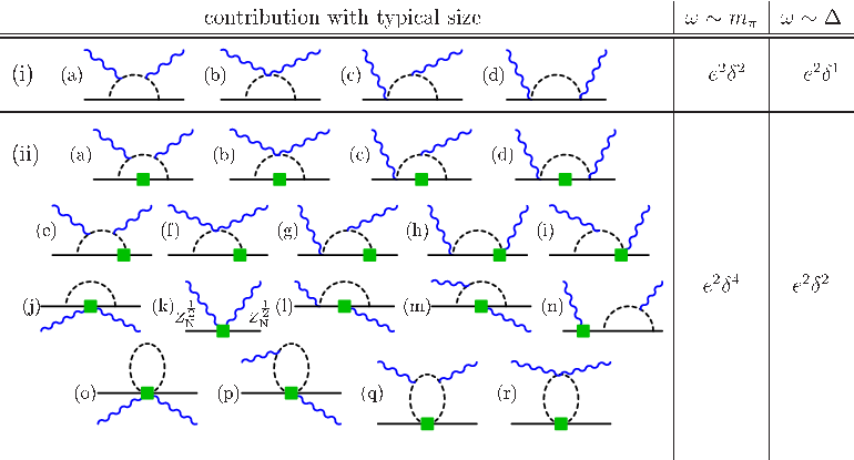
The second class of contributions comprises the pion-loop diagrams of Fig. 2. The leading contributions are and give the polarisability contributions of Eq. (1). In dimensional regularisation the full amplitude contains only two divergences at order , which are cancelled by and . The finite parts of these LECs encode contributions to the polarisabilities from mechanisms other than soft-pion loops or Delta contributions, i.e. from short-distance effects. In contrast, the spin polarisabilities are still parameter-free predictions at this order. Two- and higher-loop diagrams and contributions from higher-order Lagrangians enter only at , and are thus suppressed. (In Sec. II.4 we discuss the prescription which puts the pion-production threshold at the kinematically correct position [56, 62].)
The diagrams in the third class contain a dynamical , as listed in Fig. 3.

The propagator in these graphs is
| (10) |
where is the kinetic energy of the Delta line, which is dominantly in regime I. Since , the propagator scales as , in contrast to the nucleon propagator, , which scales as . Diagrams with a Delta are thus suppressed by one order in relative to the corresponding nucleon diagrams, and hence start at . Here, we made the argument using the heavy-baryon propagator for the Delta, as it is more transparent, even though we actually choose to compute the pole graphs using a relativistic propagator, as described in Sec. II.2.2. The loops are computed using the heavy-baryon propagator, and this ostensibly generates an inconsistency. However, the difference between the results with heavy-baryon and relativistic propagators is higher order in the expansion in , and is numerically small [68], so the inconsistency thereby introduced is insignificant.
Corrections to these Delta-contributions from add a power of and thus enter only at . There are therefore no corrections to the amplitude from effects at in this kinematic regime.
II.2.2 Regime II:
In this regime, the propagates close to its mass-shell, and its non-zero width is predominantly generated by loops. The details of the counting for this case were derived in Ref. [63] and are briefly repeated here. The leading effect comes from re-summing the leading one-Delta-reducible diagrams via a Dyson equation to obtain a dressed Delta propagator, so that Eq. (10) becomes
| (11) |
Since the kinetic energy flowing through the propagator in this region is and the vertex scales as , the leading self-energy contribution, Fig. 4, scales as .

Written as a function of Mandelstam , its imaginary part is:
| (12) |
where is the Heaviside function and the centre-of-mass momentum of the pion in the system:
| (13) |
Following Ref. [63], we keep only the imaginary part of and absorb the real part into and into the Delta wave-function renormalisation. Note that we quote the relativistic result for the Delta self energy, for reasons to be explained.
After it is dressed by the self-energy (9), the Delta propagator (11) scales as . This is different from the scaling of the propagator (10) for because as becomes comparable to , there is a region where the difference scales as . With , this is numerically the case for . For photon energies this close to the -nucleon mass-splitting, all terms in the Dyson series are of the same order, , so that the resummation of the Delta width is mandated by the power counting. This conforms with the reasoning that regime II should be limited to the region about the resonance position, with its width approximately given by the width of the resonance.
The fact that, relative to regime I, the photon energy is enhanced by one order to , and the Delta propagator near resonance is enhanced by two orders, changes the relative importance of the contributions to Compton scattering in regime II. The leading order is , and consists of the -channel tree-graph, Fig. 3(i), which contains the leading M1 coupling and the dressed propagator (12).
Since we already use the relativistic self energy, NLO () contributions to the Compton amplitude come only from Thomson “seagull” of Fig. 1(a), and from the vertex corrections, symbolically included in the shaded blob of Fig. 3(i). These appear as both loop and counterterm effects, including one coupling , and will be discussed in Sec. II.3.
In the u-channel pole and -loop graphs the Delta propagator is not enhanced, but counts as , as in regime I. These, along with the loops, all start at (N2LO) in regime II. Higher-order couplings, together with two-loop contributions, also contribute at this order.
So far our discussion of power counting has been based on HBPT. A strict application would give the peak of the resonance at , with the Breit-frame photon energy. The correct position, , would then be restored perturbatively as an expansion in . The cross section in this regime is dominated by the Delta resonance, and is very sensitive to its exact location. At a minimum, those corrections which ensure the correct real part of the resonance energy must be resumed. Doing this means that we avoid purely kinematic—and hence artificial—shifts of the polarisabilities from one order to the next. (See Sec. II.4 for the analogous procedure for the pion loops.) Note that, even with the correct real part of the resonance energy ensured, the full EFT amplitude up to NLO in the resonance region includes a number of -suppressed vertex effects. Furthermore, despite the fact that at the resonance, the strong dependence of on (see Eq. (12)) means that the relativistic and non-relativistic widths differ by a factor of 2 (for a fixed value of ).
An efficient way of dealing with these issues in practice is to use a covariant expression for the Delta-pole graphs, based on the Lagrangian [63]. This automatically takes care of both recoil and vertex corrections, by including effects which are higher-order in the power counting than the order to which we are working; except for the correct kinematics this cannot improve our agreement with data, but—as long as the power counting is valid—it should not hinder it either. In the same spirit, we also determine the resonance parameters and from the Breit-Wigner peak and width, the latter via the relativistic formula.
II.2.3 Unified description of regimes I and II
While separate sets of amplitudes for regimes I and II are possible, matching them smoothly in the transition region would be cumbersome. It is more convenient to work with one set of amplitudes which is applicable in both regimes simultaneously. We therefore choose to include all diagrams which contribute to N4LO () in regime I or to NLO () in regime II, even if they contribute at higher orders in the other regime. This is indeed the set of diagrams discussed above, Figs. 1 to 3, with a relativistically resummed Delta propagator for the tree amplitudes of Fig. 3(i). Moreover, each set is gauge and renormalisation-group invariant by itself. Therefore, adding them does not lead to conceptual problems, but neither does it improve the accuracy of the calculation. It is merely convenient to describe Compton scattering on the proton with one set of amplitudes from zero energy up to the Delta resonance. The accuracy in each regime is still given by the highest order at which all contributions are included. In regime I (), that order is or 4 orders beyond LO, and the relative systematic uncertainty of the Compton cross section can thus a priori be assessed as to . In regime II (), that is , i.e. NLO, with a relative a priori error of to .
Since the amplitudes are therefore less accurate at high energies, we choose in the following to analyse in detail the data lying in regime I, and then check the consistency with experiments in the Delta-resonance region.
We finally stress that the regimes of applicability of the different counting schemes are estimates: transition from one regime to the next is not abrupt but gradual, and the above considerations provide only typical a priori error estimates. Convergence of the EFT expansion order-by-order must be checked carefully so as to reliably assess theoretical uncertainties. Ultimately, comparison to data will help to decide whether the theory accurately describes Compton scattering.
II.3 vertex corrections
As alluded to in Sec. II.2.2, corrections which contribute to the vertices of the Delta-pole graph of Fig. 3(i) are, in the low-energy regime, of higher order than that to which we work. However in the medium-energy region they are promoted to start at NLO; see Fig. 5:

the vertex corrections are , whereas the dominant () vertex is . Thus pion-loop effects in the vertex contribute to the part of the Delta-pole graph. They are therefore predicted to be more important in the vicinity of the resonance than even the basic -loop graphs depicted in Fig. 2. Since we use EFT to fit Compton data in the resonance region—especially to constrain the M1 coupling—we include vertex loops in our calculation in order to be complete to NLO in this region. They have not been considered in recent Compton-scattering calculations [66, 67, 1], although the importance of the imaginary part of Fig. 5(ii)(b) was recognised in the original -expansion study of Ref. [63].
Inclusion of these graphs is also necessary to satisfy Watson’s theorem [79], which requires that the pion photoproduction amplitudes at the peak of the resonance are purely imaginary. This implies that the real contribution from N Born diagrams must be cancelled by Delta-pole graphs with a purely imaginary vertex that results from loops. When these elements are assembled into Compton diagrams the net effect is that, at resonance, there are cancellations between the isospin-3/2 pieces of of the loop graphs of Fig. 2 and Delta-pole graphs with imaginary vertices from the loops of Fig. 5(ii) and (iii). Diagrams which are connected in this way are shown in Fig. 6.

Since we are using heavy baryons for the calculation of the loops of Fig. 2, but the covariant version for the Delta-pole graph, we have a choice about whether or not to use the heavy-baryon expansion in computing these vertices; neither choice is fully consistent, although the inconsistencies are associated with higher-order effects in -counting. Thus we use the covariant formulation to accord with other aspects of our treatment of the Delta, such as the -loop which gives the width (see Sec. II.2.2).
Pascalutsa and Vanderhaeghen [78] computed both -loop graphs of Fig. 5 at leading order in the covariant formulation of baryon EFT. Since their calculation was reported at the peak as a function of , while we are interested in the vertices for real photons away from the peak, for completeness we give results for this case here. (Note that in Eq. (47) of Ref. [78] is a misprint for .)
Both diagrams contribute to both the structures whose coefficients are and at tree level. These corrections are labelled as () for the first diagram, Fig. 5(ii)(b), since it contains the photon coupling to the pion; and as () for the second diagram, Fig. 5(iii), since in it the photon couples to the nucleon:
| (14) |
where , , and
| (15) |
The imaginary parts of both diagrams can be calculated in closed form [78]; we have also checked them against Watson’s theorem for photoproduction. In the heavy-baryon limit, the expressions for graph (ii)(b) (in which the photon couples to the pion in the loop) agree with those obtained by Gellas et al. [75], and for (iii) (in which the coupling is to the nucleon) with our own heavy-baryon calculation—with the following proviso. In the covariant theory graphs (ii)(b) and (iii) are treated as being of the same (leading) order. However in the heavy baryon formulation (iii) is higher order, suppressed by , as is most easily seen in the gauge in which the leading photon-nucleon coupling is the magnetic one. At the same order the anomalous magnetic moment enters, so that the coupling is proportional to the total magnetic moment. Since we work to the order at which the anomalous magnetic moment enters for the direct pion loops, we do the same for the vertex loops, and multiply by the isovector Dirac magnetic moment . Furthermore, even at this order in the heavy-baryon theory, there is no contribution from graph (iii) to the electric coupling , the leading term in an expansion of from Eq. (14) being .
Following Ref. [78] we subtract from the above results the real parts at , so that the renormalised Lagrangian constants and are defined to give the real part of the dressed couplings at the pole. When we discuss fitting we mean this quantity.
However, even after such a subtraction, both contributions to contain dependences. This corresponds to a residual logarithmic dependence on the renormalisation-scale in the heavy-baryon case [75]. That could be absorbed (for (ii)(b)) by the HB Lagrangian LEC of Eq. (5), but no corresponding LEC was included in the relativistic Lagrangian of Ref. [78]. Since the expressions are finite, and we have no information on the LEC , we do not consider the additional effect from it.
In fact, in the vicinity of the resonance, the variation with of the real part of each loops graph is formally of higher order than the imaginary part (the argument parallels that of Ref. [63] when discussing the self-energy of the Delta). Moreover, the ’s also receive (real) contributions from diagrams with the same topology as diagram (ii)(b), in which the baryon propagating in the loop is a . A full computation of the vertex functions to this order is however beyond the scope of this paper. And indeed, at NNLO in this kinematic domain the Delta propagator also receives substantial two-loop corrections [80]. Therefore in what follows we discard the real part of diagram (iii), even when, working to fourth order, we retain the imaginary part for consistency with Watson’s theorem.
To summarise, therefore, the dressed vertices we use are
| (16) |
where superscripts (3) and (4) indicate use in calculations accurateÊÊin the low-energy regionÊto and respectively.

The results of this calculation are shown in Fig. 7. The first two panels depict and , with the dotted line giving the constant (tree-level) result for comparison. When the effect of diagram (ii)(b) is added the solid line is obtained (so these are ), and the dashed line is the result when the imaginary part of graph (iii) is included as well (with the factor for , giving ). We see that the hierarchy of effects predicted by the power counting (after renormalisation) indeed holds:
| (17) |
(The inverted hierarchy for the loop contributions to has a double origin: the contribution of (ii)(b) happens to be small, while the large value of makes the contribution from (iii) unnaturally large.) As for the relative size of and , the ratio of multipoles E2/M1 is
| (18) |
where
| (19) |
since the operator multiplying contains an extra time derivative. The quantity is displayed in the third panel, where the different scale on the -axis makes it clear that the effect of on observables is higher order than the constant leading term in . It was from the ratio (19), evaluated at , that Ref. [78] obtained the result . We also use that result to fix the ratio .
We emphasise that the results we obtained for the variation in the real part of with are dependent on our particular definition of Delta-pole piece. In particular, a redefinition of the field would not change the value of these functions at , but could affect their variation as we move away from the pole. Therefore the results shown in Fig. 7 only have meaning within the context of the specific and that we have adopted here.
II.4 Re-summing recoil corrections
In the heavy-baryon version of one-nucleon EFT, interactions and amplitudes are expanded in powers of . As with the correct position of the the pole discussed at the end of Sec. II.2.2, that of the one-pion production threshold is thus only reached as a perturbative expansion with higher-order terms. This has consequences for Compton scattering since the opening of the photoproduction channel induces pronounced cusps in the amplitudes, as discussed in detail in Ref. [62]. Pion production starts in Compton-scattering experiments at photon energy MeV in the lab frame. In contrast, the HB amplitude neglects recoil by assuming a nucleon which is at LO infinitely heavy, and thus puts the threshold at photon energy . The HBPT amplitude has a cusp at this point, and that at is singular there. The consequences of the cusp are seen even for below , so getting it in the right place is mandatory for an accurate description of data around the pion threshold.
Various schemes exist in the literature to correct for these purely kinematic effects by a resummation of higher-order terms that is motivated by a modified power-counting in the vicinity of a threshold (see Ref. [54] for an early discussion). All schemes agree within the order to which the EFT calculation is performed, with each effectively trying to expand the amplitudes not about but about the kinematically correct threshold position. As in Ref. [62] we replace the Breit- frame photon energy, , with the quantity , defined via:
| (20) |
This has the advantage that it implies changing the amplitude for only starting at . (Note that a slightly different substitution was adopted in Refs. [56, 57, 58]).
To preserve crossing symmetry we perform this substitution in all - and -channel (i.e. crossed) diagrams containing loops, Fig. 2. At this is all that is done. However at we need to ensure a finite amplitude as we cross the threshold. This requires that we do not double count the effects which were already included in the result via the shift (20). Thus, if the straightforwardly computed HBPT loop amplitude is (in an obvious notation) , at we compute:
| (21) |
where the superscript indicates that only the piece of the frame-dependent factor is retained. This yields a finite result for the amplitude as it crosses the cusp, and that cusp is now in the correct place regardless of the frame in which the Compton amplitude is computed [54, 56].
We note again that—as long as we are not close to the specific locations of analytic structure in the complex plane, namely the Delta pole and the cut—neither the resummation of recoil corrections to place the threshold in the right place, nor our use of a fully-covariant amplitude for the Delta-pole graphs, add any new dynamics. In the heavy-baryon expansion, all these kinematic effects reduce in either regime to corrections which are higher than the orders with which we are concerned.
II.5 Constraints from other processes and sum rules
Strictly speaking, there are two parameters at which can only be determined from proton Compton scattering: the finite part of the short-distance contributions , to the proton’s scalar electric and magnetic dipole polarisabilities. The couplings and can in principle be determined from the width and ratio of the radiative decay.
It is, however, useful to check the consistency of the values found for these parameters against other constraints. For example, the Baldin sum rule relates the sum of the scalar dipole polarisabilities at zero energy to an integral of the weighted total dissociation cross section starting at the production threshold via a dispersion relation. We use the value from the recent global fit of [33]:
| (22) |
where the canonical units, , for scalar polarisabilities, are to be understood here and below. The “recommended value” of Ref. [3], , which is based on an analysis of total photo-absorption cross sections, differs from the value (22) by less than the uncertainty in the sum-rule evaluation.
III Results
The data sets we shall use to fit our free parameters are discussed extensively in our recent review, Ref. [1]. For the reasons explained there, in the low-energy region we include data from Refs. [5, 6, 8, 9, 10, 29, 30, 31, 32, 33], but not from Refs. [4, 7]. The Baranov 150∘ data [9, 10] were also excluded. Above the photoproduction cusp, the data of Hallin [31] rises much more strongly than that of Olmos de León [33]. Hence the former was excluded from the analysis we presented in Ref. [1]. This leaves a gap in the database between MeV and MeV, so although we quote a cutoff of 170 MeV on the data set for our low-energy fits, in practice we could have chosen this to be anywhere in the range 164–198 MeV without altering the results. (For further discussion see Sec. III.3.2 below.) Below our cutoff two further points are excluded as clear outliers, namely Federspiel (, 44 MeV) and Olmos de León (, 108 MeV). For the other Olmos de León points we follow Wissmann [82] and add a point-to-point systematic error of 5% in quadrature with the statistical error for the Olmos de León data set (not shown in plots). Lastly, although we remove the data of Hallin [31] above 150 MeV, the data from this experiment at or below the photoproduction cusp are completely consistent with the rest of the database, and so, to maximise our statistical power, we include it in our fits.
We float the normalisation of each of these data sets within the quoted normalisation uncertainty, by using the standard augmented function as given in Eq. (4.19) of Ref. [1]; see Ref. [83] for more details. (The MacGibbon data [32] is counted as two data sets since the higher-energy untagged data is treated separately).
For the physical parameters in the sector of the theory we use [84] MeV, MeV, MeV, , and . For the other LECs from we use GeV-1, GeV-1 and GeV-1 [24]. 11 1 Ref. [24] gives , , , all in GeV-1, from which we subtract the Delta-pole contribution of from and respectively. The neutral pion mass MeV is used in the pole diagram but not elsewhere; other isospin-breaking effects are neglected. The Delta parameters are fit to the Breit-Wigner peak and relativistic width as MeV and .
Finally, we remind the reader that we use units of fm3 for and , and fm4 for the spin polarisabilities.
III.1 Fitting strategy
The aim of this investigation is to extend and merge the approaches of Hildebrandt et al. and Beane et al. [57, 58, 62], carrying out a definitive fit of and to low-energy data at in chiral EFT with a dynamical Delta. As summarised in Sec. II.2.3, the ingredients are as follows. Born and pion-pole graphs are included, as are counterterms for and ; see Fig. 1. In addition we add the and loops of Figs. 2 and 3. The Delta-pole graphs of Fig. 3(i) are treated covariantly, using the Lagrangian of Eq. (6) together with the corresponding expression for the width Eq. (12), and we include vertex corrections as discussed in Sec. II.3, Fig. 5. The amplitude is complete to in the low-energy region (sometimes referred to below as “fourth order”, since it corresponds to for the loops) and in the resonance region.
Hildebrandt et al. additionally fit the coupling constant to data from Refs. [31, 33] which satisfied MeV. This was done without the inclusion of any width for the . We have examined the advisability of repeating this strategy (with a Delta width included). In fits to data below about MeV, the 1--surface in the -- parameter space is large, with a particular degeneracy between and . Extending the fit to higher energies tends to constrain , but at the expense of preferring values of and which are less compatible with the low-energy values. The significance of this finding is hard to judge in view of the fact that the data set between 170 and 240 MeV is sparse and inconsistent (as discussed in detail in the review [1]).
Instead we adopted the following strategy. It clearly makes sense to use resonance-region data to determine ; the cross section there is essentially proportional to . Unlike Hildebrandt et al., our amplitude is at least NLO in this region, since we use the covariant Delta. This further has the advantage that the parameters and have the same meaning as in the photoproduction study of Pascalutsa and Vanderhaeghen [78]; we can therefore take the ratio from their work. Furthermore, though we choose to treat as a fit parameter we should get a value which agrees with Ref. [78] () up to corrections beyond NLO.
However, above 200 MeV the data sets of, on the one hand, Hallin [31] and Blanpied [40], and, on the other, Wolf [38] and Camen [39], together with others working at Mainz [34, 35, 36, 37], are too discrepant for a consistent fit to be obtained. We have chosen to use the Mainz data for our fits to the higher-energy region, for reasons discussed further in Ref. [1]. Thus we fit to Mainz data between 200 and 325 MeV, then and to world data below 200 MeV, and iterate until convergence is reached. We do not pay too much attention to the quality of the high-energy fit, since our amplitude is only NLO in this region; in addition the data are noisy and there are apparent trends in the data that are not fully reproduced. We do, however, expect a high quality of fit at low energies.
In Ref. [1] we presented an fit to the Compton database using just this strategy (note though that vertex corrections were not included in the amplitude there). The Hallin data were ultimately excluded because of their unacceptable . We obtained a good fit with a of 106.1 for 124 degrees of freedom (d.o.f.) (135 data points, 9 floating normalisations and 2 fit parameters). This calculation with the -loops computed to third-order——in the EFT expansion—sets a standard for the calculation we present here.
However simply repeating such a fit with the -loop calculation improved to fourth order does not yield an acceptable . An examination of the work of Refs. [57, 58, 62] reveals why this is the case: both the pion loops and the Delta significantly improve agreement compared to the pure third-order HBPT result by raising the cross section in the cusp region. Their combined effect raises the cross section above the data. The values of the spin polarisabilities also suggest this problem. They are significantly closer to the indicative values provided by dispersion-relation (DR) analyses in the Delta-less theory at fourth order in HBPT than they are at third order. However, adding the Delta-pole then provides a substantial additional contribution [76]. This suggests a resolution of the problem: just as adding the Delta to the Delta-less theory required the promotion of the fourth-order counterterms for and , so, when fourth-order loops and an explicit Delta are both considered, one or more of the (nominally ) counterterms for the spin polarisabilites needs to be promoted, and included in our calculation.
We have therefore explored the effect of varying each of the spin polarisabilities in turn, i.e. fitting one spin polarisability, along with and to the low-energy data. (Fits where more than one spin-polarisability is varied produce soft directions in parameter space which limit our ability to extract and with reasonable errors.) We determine the optimal spin polarisability to include amongst the fit parameters according to the following selection criteria: the low-energy should be good; the fitted value of the spin polarisability should be “sensible”—which in practice means bringing closer to than with the pure fourth-order fit; the Baldin-constrained fit should be compatible with that obtained without the constraint; and the reproduction of the high-energy data should not be badly compromised (for reasons already explained, we do not rely solely on the value to determine this). We find that on almost every count varying is superior to varying , , or ; in particular it gives the lowest low-energy . Furthermore is the spin polarisability for which the pure fourth-order prediction is most discrepant with DR estimates [2], and the only one (with an acceptable ) with a fitted value closer to the DR estimates than the unfitted one. For all those reasons we choose to fit as an additional parameter when presenting our final result. We would caution, though, that we do not regard our extracted value for this parameter as definitive, since we believe that polarised Compton scattering is a much better arena in which to explore the spin polarisabilities.
III.2 Results with the low-energy amplitude
We fit both without and with the Baldin-sum-rule constraint (see Sec. II.5). The statistical errors are obtained from the ellipsoid (ellipse). Since is fit to an independent higher-energy data set, its small statistical error in principle feeds through to produce an additional small error on the low-energy parameters, but this is negligible compared to other uncertainties.
Our result then is, for the fit without the Baldin sum rule constraint:
| (24) |
with and , as well as a of 110.5 for 134 d.o.f. For the Baldin-constrained fit, we obtain or
| (25) |
with and , with a of 113.2 for 135 d.o.f. If we instead take from Ref. [78], the Baldin-constrained value of drops only slightly from 3.15 to 3.0, well within the statistical uncertainty. In both parameter sets we have also included estimates of the individual residual theoretical uncertainties from higher-order corrections. Before we can justify them in Sec. III.3.4, we need to explore the sensitivity of the fits to choices of the parameters and data sets, as well as convergence issues.
The statistical errors are calculated from the boundaries of the ellipsoid or ellipse. In contrast, our 1 regions in 3d-parameter space are calculated according to (or for 2d), and encompass 68% of the probability. The projections of such regions in -- parameter space onto the - plane are shown in Fig. 8, together with the Baldin-constraint band. We can see that the two extractions are fully compatible with one another, as we had required for an acceptable fit. We have also checked that the is not unacceptably large for any individual data set, and that none of the normalisations floats beyond the quoted systematic error. In particular, the 65 Olmos de León points are fit with a of 69 (unconstrained) and 71 (constrained) with negligible floating of the normalisation. Our slightly restricted set of world low-energy data is clearly highly compatible, and indeed the errors on some sets seem to be overstated.

In Fig. 9 the results are shown (along with third-order fits close to those of Ref. [1] which will be discussed later), together with all the world data, including those data sets that we did not include in our fits.

As expected, the differences between constrained and unconstrained fits are small. Essentially no systematic deviation from the trend of the low-energy data is visible. The trend of the high-energy Mainz data is well captured, except for a tendency to fall somewhat low at forward angles.
For reference, with and , the other three spin-polarisabilities take the values , and (excluding the pole contribution which is -45.9 for ). See table 4.2 of the review [1] for values in other EFTs and in dispersion-relation extractions.
III.3 Further details of the fit
III.3.1 Sensitivity of the differential cross section to , , and
In Fig. 10 we show the sensitivity of the low-energy fourth-order cross section to varying within the rather wide band 3.1-4.1. Note that if is not fixed, it has a contribution from the Delta which is proportional to , and so the variation of the cross section with is somewhat larger, especially at forward angles. However, the overall scale of the effect is similar. We observe that there is virtually no sensitivity to below the cusp at more forward angles, which explains why Beane et al. [57, 58] were able to fit this region so well.

In Fig. 11 we show the sensitivity to varying within the bands 11.8-15.8 and 6-9 respecttively. We see, as expected, that most sensitivity to () occurs at forward (backward) angles. Since there is no modern data below 60∘ it is not surprising that—as can be seen from Fig. 8 and as we will discuss further in Sec. III.3.4—sensitivity to is significantly less than to , suggesting that the Baldin-constrained fits are more reliable.

Further exploration reveals that sensitivity to is almost vanishing at 90∘ even for energies up to the peak of the resonance. Of course the contribution to of Eq. (2) vanishes at this angle. However, there is a piece of , and this, in fact, is a dominant part at 90∘ in the resonance region. Nevertheless, the observation stands.
III.3.2 Choice of data set
After the elimination of inconsistent data sets, we are left with a choice of energy to define the top of the “low-energy” region. Accepting that Hallin data above the cusp cannot be accommodated means that there is no other modern data between 164 and 198 MeV, and indeed only Olmos de León data between the cusp and 164 MeV. Above 200 MeV not only is the data sparse and inconsistent, but the prominence of the Delta means that our amplitude, which is only NLO in the resonance region, is less trustworthy. So we prefer not to extend our “low-energy” fit into this region. On the other hand, since the amplitude above the cusp is markedly more different between third and fourth order than that below, a conservative choice of fit region would stop at 150 MeV—in which region the Hallin data is perfectly consistent. So to test our sensitivity to the choice of data sets and cut-off, we consider three possibilities: (I) MeV, Hallin included (137 points, 10 data sets); (II) MeV, Hallin excluded (135 points, 9 data sets); and (III) the union of both sets (147 points, 10 data sets).

Fig. 12 shows that the results from all three strategies are highly consistent; the values for in the Baldin-constrained fits, with statistical errors, are (I) , (II) , and (III) where excessive precision has been used simply to demonstrate the slight differences between the three. Though it clearly hardly matters which one we use, we choose as standard the largest data set, (III).
We also consider the effect of changing the upper cut-off on the higher-energy data to which we fit ; a cut-off of 350 MeV favours a somewhat larger of 3.69, and the Baldin-constrained in the corresponding low-energy fit drops to 3.08 (), which is clearly well within our uncertainties.
III.3.3 The effect of loop corrections to the vertices
While the the loop vertex corrections of Fig. 5 have previously been considered in photoproduction [78], this calculation is the first to include them consistently in a study of Compton scattering. Their principal effect is to generate a significant imaginary part in the vertex above the photoproduction threshold, and hence, since the Delta-pole contribution to the cross section scales as , to decrease the resonance peak height for a given (recall that is fixed to be the real part of the running coupling constant at resonance). In practice, this means that when we fit , we get a slighly higher value if the coupling runs than if it does not, somewhat reducing the slight discrepancy between the values obtained here and in Ref. [78]. A less significant effect is that the real part also runs, and we recall that this running is essentially arbitrary since there is a LEC ( of Eq. (5)) whose finite part we choose not to include.
If we fit only to data below the cusp (where the imaginary part vanishes), the and in the Baldin-constrained fit differ by less that a percent with and without running. Including the rest of the Olmos de León data, the fit without running has and (cf. and with the running), which is only a very slight change. As shown in Fig. 13, once the low-energy parameters are adjusted, the curves below the cusp with and without the running are indistinguishable by eye. In the resonance region the effects are of course more marked, and there is a modest improvement in the fit when running is included.

III.3.4 Convergence and residual theoretical uncertainties
We are now in a position to examine the convergence of our results as we go from (“third order”) to (“fourth order”) in the low-energy amplitude. The nucleon Born contribution changes appreciably between these two, whereas the difference between the fourth-order result and the fully covariant amplitude is negligible, so we choose to use the fourth-order Born for both amplitudes, just as we use the covariant Delta-pole graphs. (Since the fourth-order Born amplitude has polarisability-like terms, the main effect of this is to avoid a spurious shift in polarisabilities between orders.) Hence the only difference between the two orders (apart from the vertex corrections) is the graphs of Fig. 2(ii). These are of two kinds: corrections to the graphs of Fig. 2(i), which would be considered part of the third-order calculation in a covariant formulation, and contributions from the second-order LECs and , which are fourth-order in both heavy-baryon and covariant formulations. Fig. 14 shows the comparison between third order, fourth order with the LECs set to zero, and full fourth order, all with the same values of the polarisabilities , . (Of course we do not switch off in the Born terms in the first two calculations, only in the loops.)

We do not show the effects of the ’s and separately, as the former is almost completely negligible. (Recall that in the theory with an explicit Delta the ’s have to be readjusted, and are all rather small.) On the other hand has an appreciable effect (largely due to ; is small). The convergence is very satisfactory up to about 300 MeV, with the difference between the third and fourth orders only exceeding 10% where the third order is anomalously low, i.e. for forward angles at the cusp. We also see that the effect of is, in the same range, of the same size as that of corrections. Hence there seems little to be gained in using a covariant formulation for the loops without including anomalous-magnetic-moment effects in the loop calculation too. Unsurprisingly, the situation is different in the resonance region, where the corrections are becoming large.
This convergence is very satisfactory from a formal perspective. However, quite a lot of the low-energy data lie in the region where the difference between the third- and fourth-order amplitudes is accidentally enhanced, and so identical results when one fits the polarisabilities to the data are not guaranteed. To test the convergence of the fourth-order results of section III.2 we perform a fit using the third-order amplitude, obtaining the following results:
| (26) |
with and of 118.6 for 134 d.o.f., and for the Baldin-constrained fit
| (27) |
with and of 120.3 for 135 d.o.f.
The total is distinctly higher than for the fourth-order fit of Eqs. (25), (24) but entirely acceptable; the preferred normalisation shift for the Hallin data is slightly greater than the systematic error of 4%, but omitting the data set has little effect on the fit parameters. This fit is shown together with the fourth-order one in Fig. 9. In the review [1] we performed third-order fits without running couplings and excluding all Hallin data; for the Baldin-constrained fit identical values were obtained, while for the unconstrained fit the results were and .

The curves for the third- and fourth-order fits together are shown in Fig. 15. We see that the results are fully in agreement with one another. The range of accommodated in each fit is quite large, and they only just overlap at the 1- level. This can be explained by the fact, noted earlier, that the two cross sections differ most at forward angles near the cusp, which is also where the sensitivity to is greatest, but there is little data at angles .
In contrast, the central values of in both fits are extremely close, and neither changes appreciably when the Baldin constraint is imposed. In view of this, we prefer to quote the fourth-order Baldin-constrained values of Eq. (25) as our final result.
Finally, we can now return to the issue of the theoretical accuracy of the extractions at in Eqs. (24) and (25) in Sec. III.2. Since the polarisabilities first enter at with the parameter-free prediction of Eq. (1), we expect corrections to be a priori of order relative to the LO result. With an average value to set the scale and , this leads to an error of (rounded up) for the individual polarisabilities of the free fit, or for the combination of the Baldin-constrained fit.
To validate this naive dimensional estimate, we can check the convergence pattern from order to order, which is predicted to be from LO to NLO and from LO to NLO. For the free fit, changes from LO to NLO by units, and from NLO to N2LO by units, while changes in each case by units, respectively. These are quite compatible with the power counting, and suggest an error on the fourth-order fit values of . To be conservative, this is what we quote on our non-Baldin-constrained fit (24).
However, Fig. 15 shows that the convergence for seems to be much better than for , the latter being poorly constrained by the data. Judging by the shift from third to fourth order, the error on could be taken to be as large as , while that on would be neglible. To estimate the error on the latter, therefore, we prefer to take times the LO-to-NLO change of , giving , and hence an error of on the Baldin-constrained values of and separately. This also implies that the theory uncertainties for the free fit of and are highly correlated.
A further way of estimating errors in an EFT is to look at the effect of the inclusion of partial higher-order terms. We have done this in the low energy region when we include the vertex corrections of Section II.3. The results for and with and without these corrections differ typically by about . From Fig. 14 we might speculate that loops with two insertions of may in fact be the dominant correction at N3LO, but still this is a reassuring result which suggests that our theory errors are not underestimated.
For the errors on the third-order results of Eqs. (26) and (27), we take the as estimated in the review [1], values which are entirely compatible with the current analysis though almost certainly too large for the Baldin-constrained results.
We close by pointing out that the statistical and residual theoretical uncertainties in extracting proton polarisabilities are now compatible.
IV Summary and Outlook
In this work we have presented a chiral effective theory analysis of scattering data. We employed an EFT with explicit nucleon, pion, and Delta degrees of freedom, arranged according to an expansion in the small parameter [63].
The EFT amplitude accurate up to in the low-energy () region was used (where the leading, Thomson, amplitude is ). This includes the fourth-order loops of Ref. [56], the loops first computed in Ref. [61], as well as Delta-pole graphs. At this order short-distance pieces of the proton scalar polarisabilities, and , appear in the Compton amplitude and these, together with the M1 transition strength, , are the free parameters in our EFT description of scattering for . However, instead of fitting in this low-energy region, we determine it using data up to MeV and a EFT amplitude which includes all (next-to-leading order) effects in the resonance region. Meanwhile, and were fit to a statistically consistent Compton database that covers the domain MeV. Fits to this database and to resonance-region data were iterated until convergence was achieved. This does not, however, result in an accurate description of data in the low-energy region. By including the short-distance piece of the proton spin polarisability, —nominally a higher-order effect in EFT—in our amplitude we obtain an excellent fit to the low-energy data. is the only spin polarisability where such promotion yields a fit that is consistent with other constraints, and with the fit presented in Ref. [1]. Since there is little data at forward angles, and it is there that the differential cross section is most sensitive to , we use the Baldin-sum-rule evaluation from Ref. [33] to constrain this combination of polarisabilities.
The resulting fit has a of 113.2 for 135 d.o.f. We find, in the canonical units of ,
| (28) |
with and . The result for is very close to that extracted using the amplitude, and is stable under modifications of the database and the inclusion of certain higher-order corrections to the vertex. Importantly, the value of obtained in this fit is consistent with that found in the pion electroproduction study of Ref. [78] at the expected level of accuracy of both calculations (NLO).
Eq. (28) presents a considerably larger value of than has been found in dispersion-relation extractions of proton polarisabilites from a similar database (see, e.g., Ref. [2]). Since is a free parameter in dispersion-relation fits, it would be interesting to know if such fits can tolerate the values of found here—and, if they cannot, what additional physics in the dispersion-relation calculation forces to smaller values. We observe that a calculation in a variant of EFT that does not use the heavy-baryon expansion predicts [66, 67]. This is consistent with our extraction (28), but disagrees with the dispersion-relation results in Refs. [2, 33].
The EFT calculation in the resonance region could be improved to NNLO by including further corrections to the vertex and computing the pertinent pieces of the two-loop self-energy of the Delta in EFT [80]. This would be particularly interesting for the development of a consistent EFT description of pion-nucleon scattering, pion photoproduction, and Compton scattering in the resonance region. The Baldin sum-rule value obtained in Ref. [33] should perhaps also be re-assessed, since slightly different values have been obtained by other groups [28, 85]. The uncertainty on the value of obtained in this way is on the verge of becoming a significant component in the overall uncertainty in and . Meanwhile, if the amplitude in the low-energy region were to be improved, a calculation beyond in the expansion would have to be carried out, and we note that graphs with two N loops enter at . As the result (28) makes clear, at this stage the theory error is slightly smaller than the statistical error, and so it seems that the accuracy with which and are known can be more profitably improved by focusing effort in other areas.
In particular, if more data were available between N threshold and the resonance then we could extend the low-energy fit region and obtain tighter constraints on and . The data that exist here are sparse, and different experiments are not consistent with one another. In consequence our database has a sizable gap between MeV and MeV. Data of high precision in this kinematic domain, with well-documented systematic uncertainties, could help reduce the statistical errors on . Indeed, if such experiments extended into the resonance region they might help to discriminate between the conflicting results of, on the one hand, Hallin [31] and Blanpied [40], and, on the other, Wolf [38], Camen [39], and other groups at Mainz [34, 35, 36, 37].
Ongoing experiments to measure asymmetries at – MeV (MAMI, Mainz) and MeV (HIS, TUNL), and thereby extract spin polarisabilities, will provide additional testing grounds for our approach [41, 42]. Meanwhile, new data on absolute cross sections from 120–180 MeV will supplement the current database, and, if sufficiently precise, aid the extraction of [43].
In fact, the EFT amplitude developed here is highly successful in reproducing extant Compton differential-cross-section data. Perusal of Fig. 9 shows that it describes experiment over a wide range of energies and angles. This is possible because the amplitude contains the key non-analyticities in scattering below MeV: the pion photoproduction cusp and the resonance pole. This benefit comes at a price, though: the chiral dynamics encoded in these non-analyticities describes data so well that effects due to short-distance physics play a relatively small role. Consequently, we had to exercise significant care in the treatment of (sometimes discrepant) data, and also consistently incorporate a number of subtle effects in the p amplitude to obtain accurate values for and .
Acknowledgments
DRP thanks the Theoretical Physics Group at the University of Manchester for their hospitality during his time that much of this work was done. We also acknowledge the organisers and participants of the INT workshop 08-39W: “Soft Photons and Light Nuclei” and of the INT programme 10-01: “Simulations and Symmetries”, both of which also provided financial support. We are grateful to Jerry Feldman, Vladimir Pascalutsa and Mike Birse for useful discussions. This work has been supported in part by UK Science and Technology Facilities Council grants ST/F012047/1, ST/J000159/1 (JMcG) and ST/F006861/1 (DRP), by the US Department of Energy under grants DE-FG02-93ER-40756 (DRP) and DE-FG02-95ER-40907 (HWG), by US National Science Foundation Career award PHY-0645498 (HWG), by the Deutsche Forschungsgemeinschaft and the National Natural Science Foundation of China through funds provided to the Sino-German CRC 110 “Symmetries and the Emergence of Structure in QCD” (HWG), and by University Facilitating Funds of the George Washington University (HWG).
Appendix A Details of the amplitudes
The nucleon Born diagrams calculated to fourth order are as given by McGovern [56]; they are indistinguishable from the full relativistic form given by Babusci et al. [71] for the energies of interest. They are obtained from the diagrams of Fig. 1; the third-order vertex represented by a triangle employs terms given in Eqs. (3.8) and (3.9) of Ref. [73]; the divergences represented by and in the latter renormalise in Fig. 2(ii)(k) and the loop in (m).
The fourth-order vertex represented by a diamond in Fig. 1(iii)(b) contributes to both the Born amplitude and to the polarisabilities. The LECs and of Eq. (3) result from linear combinations of the fourth-order operators to , and of Ref. [73]. The Born amplitudes also involve fixed-coefficient parts of these (table 6 of [73]) together with those of the operators , and . The relevant -functions are those of to , , , and of Ref. [74] (though there would seem to be a misprint in one or more of the “eye-graph” contributions as the divergence cancellation for does not quite work.)
The pion-pole contributions are given by Bernard et al. [21]; this form does not change at fourth order and is indeed relativistically invariant, although at fifth order form factors will enter at the vertices, and the LEC shifts to the numerically almost identical .
The loops of Fig. 2 are given at third order by Bernard et al. [21] and at fourth order by McGovern [56]. At both third and fourth order, we use to shift the threshold to the correct energy, as detailed in Sec. II.4. The loops are given by Hildebrandt et al. [62] in their Appendix B, except that we use the Breit-frame photon energy throughout in place of and to preserve crossing symmetry.
The - and -channel Delta-pole diagrams are calculated using the Lagrangian of Pascalutsa and Phillips [63]. The expressions for the Delta-pole amplitudes given in Eqs (A3) and (A4) of that paper refer to a redundant, covariant set of eight operators. We note that the correct forms of three of these are
| (29) |
the others are given in their Eq. (51). Other misprints in Ref. [63] are noted in Ref. [1]; in particular the expression for the width given in their Eq. (42) is a misprint for our Eq. (12). These eight operators may be written in terms of the six Breit frame operators of Eq. (2), which we will denote (with e.g. ) using
| (30) |
where
| (31) |
is the Breit-frame nucleon energy, , and .
References
- [1] H. W. Grießhammer, J. A. McGovern, D. R. Phillips and G. Feldman, Prog. Part. Nucl. Phys. 67 (2012) 841.
- [2] D. Drechsel, B. Pasquini and M. Vanderhaeghen, Phys. Rept. 378 (2003) 99.
- [3] M. Schumacher, Prog. Part. Nucl. Phys. 55 (2005) 567.
- [4] C. L. Oxley, Phys. Rev. 110 (1958) 733.
- [5] L. G. Hyman, R. Ely, D. H. Frisch and M. A. Wahlig, Phys. Rev. Lett. 3 (1959) 93.
- [6] V. I. Gol’danskii et al., Sov. Phys. JETP 11 (1960) 1223.
- [7] G. Bernardini et al. Nuovo Cimento 18 (1960) 1203.
- [8] G. Pugh et al., Phys. Rev. 105 (1957) 982 and references therein; MIT Summer study 1967 p. 555.
- [9] P. S. Baranov et al., Phys. Lett. B 52 (1974) 122.
- [10] P. S. Baranov et al., Sov. J. Nucl. Phys. 21 (1975) 355.
- [11] J. W. DeWire, M. Feldmann, V. L. Highland, R. Littauer Phys. Rev. 124 (1961) 909.
- [12] P. S. Baranov, L. I. Slovokhotov, G. A. Sokol and L. N. Shtarkov, Sov. Phys. JETP 23 (1966) 242.
- [13] P. S. Baranov et al, Sov. J. Nucl. Phys. 3 (1966) 791.
- [14] E. R. Gray and A. O. Hanson, Phys. Rev. 160 (1967) 1212.
- [15] H. Genzel, M. Jung, R. Wedemeyer et al., Z. Phys. A279 (1976) 399.
- [16] S. Weinberg, Physica A 96 (1979) 327.
- [17] J. Gasser and H. Leutwyler, Phys. Rept. 87 (1982) 77.
- [18] J. Gasser and H. Leutwyler, Annals Phys. 158 (1984) 142.
- [19] E. E. Jenkins and A. V. Manohar, lectures at “Workshop on Effective Field Theories of the Standard Model”, Dobogoko, Hungary, Aug 1991. In “Dobogokoe 1991, Proceedings, Effective field theories of the standard model”, pp. 113-137.
- [20] E. E. Jenkins and A. V. Manohar, Phys. Lett. B 259 (1991) 353.
- [21] V. Bernard, N. Kaiser and U.-G. Meißner, Int. J. Mod. Phys. E 4 (1995) 193.
- [22] S. Scherer, Adv.. Nucl. Phys. 27 (2003) 277.
- [23] V. Bernard and U.-G. Meißner, Ann. Rev. Nucl. Part. Sci. 57 (2007) 33.
- [24] V. Bernard, Prog. Part. Nucl. Phys. 60 (2008) 82.
- [25] S. Scherer and M. R. Schindler, Quantum chromodynamics and chiral symmetry, Lect. Notes Phys. 830 (2012) 1. (Springer)
- [26] V. Bernard, N. Kaiser, J. Kambor and U.-G. Meißner, Nucl. Phys. B 388 (1992) 315.
- [27] V. Bernard, N. Kaiser, and U.-G. Meißner, Phys. Rev. Lett. 67 (1991) 1515.
- [28] D. Babusci, G. Giordano, G. Matone, Phys. Rev. C57 (1998) 291.
- [29] F. J. Federspiel, R. A. Eisenstein, M. A. Lucas et al., Phys. Rev. Lett. 67 (1991) 1511.
- [30] A. Zieger, R. Van de Vyver, D. Christmann, A. De Graeve, C. Van den Abeele and B. Ziegler, Phys. Lett. B 278 (1992) 34.
- [31] E. L. Hallin et al., Phys. Rev. C 48 (1993) 1497.
- [32] B. E. MacGibbon, G. Garino, M. A. Lucas, A. M. Nathan, G. Feldman and B. Dolbilkin, Phys. Rev. C 52 (1995) 2097.
- [33] V. Olmos de León et al., Eur. Phys. J. A 10 (2001) 207.
- [34] C. Molinari et al., Phys. Lett. B 371 (1996) 181.
- [35] J. Peise et al., Phys. Lett. B 384 (1996) 37.
- [36] A. Hünger et al., Nucl. Phys. A 620 (1997) 385.
- [37] F. Wissmann et al., Nucl. Phys. A 660 (1999) 232.
- [38] S. Wolf et al., Eur. Phys. J. A 12 (2001) 231.
- [39] M. Camen et al., Phys. Rev. C 65 (2002) 032202.
- [40] G. Blanpied et al., Phys. Rev. C 64 (2001) 025203
- [41] R. Miskimen, talk at Conference on Intersections of Particle and Nuclear Physics, St. Petersburg, FL, May 2012, to appear in the proceedings.
- [42] R. Miskimen et al., HIGS Proposal P-06-09, Measuring the Spin Polarizabilities of the Proton in Double-Polarized Real Compton Scattering (2009).
- [43] D. Hornidge, talk at Conference on Intersections of Particle and Nuclear Physics, St. Petersburg, FL, May 2012, to appear in the proceedings.
- [44] W. Detmold, B. C. Tiburzi and A. Walker-Loud, Phys. Rev. D 73 (2006) 114505.
- [45] W. Detmold, B. C. Tiburzi and A. Walker-Loud, Phys. Rev. D 79 (2009) 094505.
- [46] W. Detmold, B. C. Tiburzi and A. Walker-Loud, Phys. Rev. D 81 (2010) 054502.
- [47] M. Engelhardt, PoS LATTICE 2011 (2011) 153.
- [48] M. Lujan, A. Alexandru and F. Lee, PoS LATTICE 2011 (2011) 165.
- [49] K. Pachucki, Phys. Rev. A 60 (1999) 3593.
- [50] C. E. Carlson and M. Vanderhaeghen, arXiv:1109.3779 [physics.atom-ph].
- [51] M. C. Birse and J. A. McGovern, Eur. Phys. J. A 48 (2012) 120.
- [52] D. R. Phillips, J. Phys. G 36 (2009) 104004.
- [53] A. Walker-Loud, C. E. Carlson and G. A. Miller, Phys. Rev. Lett. 108 (2012) 232301.
- [54] V. Bernard, N. Kaiser, A. Schmidt and U.-G. Meißner, Phys. Lett. B 319 (1993) 269; Z. Phys. A 348 (1994) 317.
- [55] S. Ragusa, Phys. Rev. D 47 (1993) 3757.
- [56] J. A. McGovern, Phys. Rev. C 63 (2001) 064608.
- [57] S. R. Beane, M. Malheiro, J. A. McGovern, D. R. Phillips, and U. van Kolck, Phys. Lett. B 567 (2003) 200 [Erratum-ibid. 607 (2005) 320].
- [58] S. R. Beane, M. Malheiro, J. A. McGovern, D. R. Phillips, and U. van Kolck, Nucl. Phys. A 747 (2005) 311.
- [59] T. R. Hemmert, B. R. Holstein and J. Kambor, Phys. Lett. B 395 (1997) 89.
- [60] T. R. Hemmert, B. R. Holstein and J. Kambor, J. Phys. G 24 (1998) 1831.
- [61] T. R. Hemmert, B. R. Holstein, J. Kambor, Phys. Rev. D 55 (1997) 5598.
- [62] R. P. Hildebrandt, H. W. Grießhammer, T. R. Hemmert and B. Pasquini, Eur. Phys. J. A 20 (2004) 293.
- [63] V. Pascalutsa and D. R. Phillips, Phys. Rev. C 67 (2003) 055202.
- [64] T. Becher and H. Leutwyler, Eur. Phys. J. C 9 (1999) 643.
- [65] T. Fuchs, J. Gegelia, G. Japaridze and S. Scherer, Phys. Rev. D 68 (2003) 056005.
- [66] V. Lensky and V. Pascalutsa, Pisma Zh. Eksp. Teor. Fiz. 89 (2009) 127.
- [67] V. Lensky and V. Pascalutsa, Eur. Phys. J. C 65 (2010) 195.
- [68] V. Lensky, J. A. McGovern, D. R. Phillips and V. Pascalutsa, Phys. Rev. C 86 (2012) 048201.
- [69] J. A. McGovern, H. W. Grießhammer, D. R. Phillips and D. Shukla, PoS CD 09 (2009) 059.
- [70] D. R. Phillips, J. A. McGovern and H. W. Grießhammer, talk at Conference on Intersections of Particle and Nuclear Physics, St. Petersburg, FL, May 2012, to appear in the proceedings. [arXiv:1210.3577]
- [71] D. Babusci, G. Giordano, A. I. L’vov, G. Matone and A. M. Nathan, Phys. Rev. C 58 (1998) 1013.
- [72] H. W. Grießhammer and T. R. Hemmert, Phys. Rev. C 65 (2002) 045207.
- [73] N. Fettes, U.-G. Meißner, M. Mojžiš, and S. Steininger, Annals Phys. 283 (2000) 273 [Erratum-ibid. 288 (2001) 249].
- [74] U.-G. Meißner, G. Müller, and S. Steininger, Annals Phys. 279 (2000) 1.
- [75] G. C. Gellas, T. R. Hemmert, C. N. Ktorides and G. I. Poulis, Phys. Rev. D 60 (1999) 054022.
- [76] T. R. Hemmert, B. R. Holstein, J. Kambor and G. Knochlein, Phys. Rev. D 57 (1998) 5746.
- [77] R. P. Hildebrandt, Ph. D. Thesis, TU München (2005), nucl-th/0512064.
- [78] V. Pascalutsa and M. Vanderhaeghen, Phys. Rev. D 73 (2006) 034003.
- [79] K. M. Watson, Phys. Rev. 95 (1954) 228.
- [80] B. Long and U. van Kolck, Nucl. Phys. A 840 (2010) 39.
- [81] B. Pasquini, P. Pedroni, D. Drechsel, Phys. Lett. B687 (2010) 160.
- [82] F. Wissmann, Compton Scattering: Investigating the Structure of the Nucleon with Real Photons, Springer Tracts in Modern Physics, Volume 200 (2004).
- [83] P. S. Baranov, A. I. Lvov, V. A. Petrunkin and N. L. Shtarkov, Phys. Part. Nucl. 32 (2001) 376.
- [84] J. Beringer et al. (Particle Data Group), Phys. Rev. D86 (2012) 010001.
- [85] M. I. Levchuk and A. I. L’vov, Nucl. Phys. A 674 (2000) 449.