Observational Constraints on Quintessence: Thawing, Tracker, and Scaling models

For thawing models of quintessence the field $\phi$ is nearly frozen in the early matter era because of the Hubble friction, so that $w$ is close to $-1$. One can regard $w=-1$ as the fixed point of Eq. (5). For $\lambda\neq 0$ such a point is not stable, and hence $w$ starts to grow at the late cosmological epoch.

If we assume that $\lambda$ is nearly constant, one can express $w$ in terms of $\Omega_{\phi}$ by using Eqs. (5) and (6) under the approximation $|1+w|\ll 1$ [27]. This neglects the effect of the field mass squared $V_{,\phi\phi}$, but it is possible to derive a more elaborate form of $w$ with the mass term taken into account [25, 26]. In doing so, the potential is expanded around the initial field value $\phi_{i}$ up to second order, i.e., $V(\phi)=\sum_{n=0}^{2}V^{(n)}(\phi_{i})\,(\phi-\phi_{i})^{n}/n!$.

Provided that $|w+1|\ll 1$, the evolution of the scale factor can be approximated by that of the $\Lambda$CDM model, i.e., $a(t)=\left[(1-\Omega_{\phi 0})/\Omega_{\phi 0}\right]^{1/3}\sinh^{2/3}(t/t_{\Lambda})$, where $t_{\Lambda}=2M_{\rm pl}/\sqrt{3V(\phi_{i})}$ and $\Omega_{\phi 0}$ is the today’s density parameter of quintessence. On using this solution, Eq. (3) is integrated to give the field in terms of the function of $t$ and hence the field equation of state $w(t)\simeq-1+\dot{\phi^{2}}/V(\phi_{i})$ is known. This process leads to the following analytic expression of $w$ [25, 26]:

where $w_{0}$ is the value of $w$ today, and

The solution (8) is valid for $K^{2}>0$. The equation of state (8) is expressed in terms of the three parameters $w_{0}$, $\Omega_{\phi 0}$, and $K$.

As a concrete example, let us consider the hilltop potential

In this case the parameter (9) is given by

If $0<\phi_{i}/f<\pi/2$ and $\pi/2<\phi_{i}/f<\pi$, one has $K>1$ and $K<1$ respectively. In the former case the potential is approximately given by $V(\phi)\approx 2\Lambda^{4}[1-\phi^{2}/(4f^{2})]$ around $\phi=0$, whereas in the latter case it is approximated as $V(\phi)\approx\Lambda^{4}(\phi-\pi f)^{2}/(2f^{2})$ around $\phi=\pi f$.

In Fig. 1 we plot the numerical evolution of $w$ versus $a$ for $K>1$ with several different values of $f$ and $\phi_{i}$. The bald dashed curves correspond to the results derived by the analytic expression (8), which show good agreement with the numerically integrated solutions for $w_{0}\lesssim-0.3$. For $K$ larger than 10, the initial displacement of the field is required to be close to $0$ to avoid its rapid roll down. In such cases the field mass is largely negative, which leads to the tachyonic instability of field perturbations. If the field reaches the potential minimum by today and it starts to oscillate, numerical simulations show that Eq. (8) is no longer reliable. We set the prior $K<10$ in the likelihood analysis of Sec. III.1.

The analytic estimation (8) starts to lose accuracy for $K$ smaller than 1. This reflects the fact that the field is initially located away from the potential maximum. Then the Taylor expansion around $\phi=\phi_{i}$ tends to be more inaccurate because of the rapid variation of the field. Numerically we find that the analytic solution (8) is reliable for $0.5\lesssim K<1$ and $w_{0}\lesssim-0.8$.

In Eq. (5) there is another fixed point given by

along which $w$ is constant. This corresponds to the tracker that attracts the solutions with different initial conditions to a common trajectory. The condition under which the tracking occurs is [19]²² 2 A similar condition for the k-essence Lagrangian $P(\phi,X)=V(\phi)W(X)$ with $X=\dot{\phi}^{2}/2$ is given by $\Gamma>3/2$ [37].

In this case the variable $\lambda$ approaches 0.

From (13) it follows that $\Omega_{\phi}^{\prime}/\Omega_{\phi}=-2\lambda^{\prime}/\lambda$. Using this relation with Eqs. (6) and (7) in the regime $\Omega_{\phi}\ll 1$, the field equation of state along the tracker is given by

For the potential $V(\phi)=M^{4+p}\phi^{-p}$ ($p>0$) one has $\Gamma=1+1/p$ and hence $w_{(0)}=-2/(p+2)$ [19, 34].

The result (15) was derived by neglecting the contribution of $\Omega_{\phi}$, but its effect can be accommodated by dealing with $\Omega_{\phi}$ as a perturbation to the 0-th order solution (15) [33]. We consider the first-order perturbation $\delta w$ around $w_{(0)}$ and then approximate $\Omega_{\phi}(a)$ by the 0-th order solution

For the models in which $\Gamma$ is nearly constant, we obtain the following analytic solution [33]:

where in the second and third lines we carried out the expansion $(\Omega_{\phi}(a)/(1-\Omega_{\phi}(a)))^{n}=\Omega_{\phi}(a)^{n}(\sum_{m=0}^{\infty}\Omega_{\phi}(a)^{m})^{n}$. The equation of state (18) is expressed in terms of the two parameters $w_{(0)}$ and $\Omega_{\phi 0}$. Numerically we confirm that the approximated formula (18) tends to approach the full numerical solution by adding higher-order terms of $\Omega_{\phi}(a)$.

The scaling solution [20] is a special case of a tracker along which $\Omega_{\phi}$ in Eq. (13) is constant with $0<\Omega_{\phi}<1$. From Eq. (6) it then follows that $w=0$ and hence $\Omega_{\phi}=3/\lambda^{2}$ during the matter era. Since $\lambda$ is constant, one has $\Gamma=1$ from Eq. (7). This corresponds to the exponential potential $V(\phi)=V_{0}e^{-\lambda\phi/M_{\rm pl}}$, where $V_{0}$ is a constant³³ 3 For the k-essence Lagrangian $P(\phi,X)$ (where $X=-g^{\mu\nu}\partial_{\mu}\phi\partial_{\nu}\phi/2$) the condition for the existence of scaling solutions restricts the Lagrangian in the form $P=X\,g(Y)$, where $g$ is an arbitrary function in terms of $Y=Xe^{\lambda\phi/M_{\rm pl}}$ [38]. Quintessence with the exponential potential corresponds to the choice $g(Y)=1-V_{0}/Y$. . In this case, however, the field equation of state is the same as that of the background fluid ($w=0$), so that the system does not enter the phase of cosmic acceleration.

This problem can be circumvented for the following model [21]

where $\lambda_{i}$ and $V_{i}$ ($i=1,2$) are constants. If $\lambda_{1}\gg 1$ and $\lambda_{2}\lesssim 1$ then the solution first enters the scaling regime characterized by $\Omega_{\phi}=3(1+w_{m})/\lambda_{1}^{2}$, where $w_{m}$ is the equation of state of the background fluid. From the bound coming from big bang nucleosynthesis [39] there is a constraint $\Omega_{\phi}<0.045$ (95 % CL) during the radiation era ($w_{m}=1/3$), which translates into the condition $\lambda_{1}>9.4$. The scaling matter era ($\Omega_{\phi}=3/\lambda_{1}^{2}$, $w=0$) is followed by the dark energy dominated epoch driven by the presence of the potential $V_{2}e^{-\lambda_{2}\phi/M_{\rm pl}}$. If $\lambda_{2}^{2}<3$, the solution approaches another attractor characterized by $\Omega_{\phi}=1$ and $w=-1+\lambda_{2}^{2}/3$ [20]. The cosmic acceleration occurs for $\lambda_{2}^{2}<2$.

The onset of the transition from the scaling matter era to the dark energy dominated epoch depends on the parameters $\lambda_{1}$, $\lambda_{2}$, and $V_{2}/V_{1}$. Numerically we find that the transition redshift is not very sensitive to the choice of $V_{2}/V_{1}$, so we study the case $V_{2}=V_{1}$. In Fig. 2 we plot the numerical evolution of $w$ for $\lambda_{2}=0$ with three different values of $\lambda_{1}$. For larger $\lambda_{1}$ the transition to the dark energy dominated epoch occurs earlier.

It is possible to accommodate the above variation of $w$ analytically by using the parametrization proposed by Linder and Huterer [40] (see also Refs. [41]):

where $w_{p}$ and $w_{f}$ are asymptotic values of $w$ in the past and future respectively, $a_{t}$ is the scale factor at the transition, and $\tau$ describes the width of the transition. The scaling solution during the matter era corresponds to $w_{p}=0$. For $\lambda_{2}=0$ one has $w_{f}=-1$, so that the parametrization (20) reduces to $w(a)=-1+[1+(a/a_{t})^{1/\tau}]^{-1}$. Figure 2 shows that the parametrization (20) can fit the numerical evolution of $w$ very well for appropriate choices of $a_{t}$ and $\tau$. For $\lambda_{2}=0$ the transition width is around $\tau\approx 0.33$, while $a_{t}$ depends on the values of $\lambda_{1}$. In this case one can carry out the likelihood analysis by fixing $\tau=0.33$ and find the constraints on $a_{t}$ (see Ref. [42] for a related work).

If $\lambda_{2}\neq 0$, then the field equation of state finally approaches the value $w=-1+\lambda_{2}^{2}/3$. Numerically we find that $w$ tends to have a minimum for larger $\lambda_{2}$ before the solutions reach the attractor. If $\lambda_{1}=20$, for example, the minimum appears for $\lambda_{2}\gtrsim 0.3$ (see Fig. 3). In order to place observational bounds on $\lambda_{2}$ in such cases, we need to resort to numerical simulations without using the parametrization (20).

Let us study observational constraints on thawing models given by the equation of state (8). Since $K$ is weakly constrained in the three-parameter analysis, we first study this model by fixing the value of $K$ and vary the two parameters $w_{0}$ and $\Omega_{\phi 0}$. This is the approach taken by Dutta and Scherrer [25]. However, because of a mild dependence (i.e. degeneracy) of the $\chi^{2}$ as a function of the parameter $K$, we will also perform the data analysis by marginalizing the $\chi^{2}$ over $K$ itself. This last procedure allows us, by hiding the information of $K$, to understand the measured parameters $\Omega_{\phi 0}$ and $w_{0}$ easily.

Although quintessence corresponds to the case $w_{0}>-1$, we also extend to the regime $w_{0}<-1$ in the likelihood analysis. In fact it was shown in Ref. [50] that the equation of state of a phantom scalar field can be accommodated by the analytic formula (8). The likelihood results are quite different depending on whether the recent BAO data from BOSS [29] are included or not, so we present two constraints with/without the BOSS data.

Let us first focus our analysis on some particular values of $K$, which allow us to make comparison with the results given in [25]. Our numerical analysis gives that, in the absence of the BOSS BAO data, the dark energy equation of state today is constrained to be $-1.219<w_{0}<-0.930$ (at 95 % CL for $K=1.01$). Dutta and Scherrer [25] showed that even the value $w_{0}=-0.7$ is allowed from the SN Ia data alone. Adding the WMAP7 and SDSS7 data gives rise to much tighter bounds on $w_{0}$. This is the case for $\Omega_{\phi 0}$ as well. We obtained the bound $0.7078<\Omega_{\phi 0}<0.740$ (95 % CL for $K=1.01$), whereas the values $0.68<\Omega_{\phi 0}<0.8$ are allowed in Ref. [25].

We also study the same case with the latest BOSS data. Having so far fixed $K$, by studying the $\chi^{2}$ over the parameter space of the remaining two parameters, we find that $w_{0}$ and $\Omega_{\phi 0}$ are constrained to be $-1.242<w_{0}<-0.995$ and $0.705<\Omega_{\phi 0}<0.734$, respectively, at 95 % CL for $K=1.01$. Rather surprisingly, the allowed parameter space in the regime $w_{0}\geq-1$ is very narrow. In particular the $\Lambda$CDM model, which corresponds to $w_{0}=-1$, is outside the $1\sigma$ observational contour. This comes from the fact that the BOSS data (32) does not allow a large parameter space with $w>-1$ at the redshift $z=0.57$.

We have also studied the case $K=4$ and derived bounds for $w_{0}$ and $\Omega_{\phi 0}$. Without the BOSS data we obtain the bounds $-1.408<w_{0}<-0.855$ and $0.711<\Omega_{\phi 0}<0.740$ (95 % CL, $K=4$), whereas with the BOSS data these parameters are constrained to be $-1.460<w_{0}<-0.982$ and $0.709<\Omega_{\phi 0}<0.734$ (95 % CL, $K=4$) respectively. In the former case the upper bound of $w_{0}$ gets larger than that for $K=1.01$. This reflects the fact that $w$ changes more rapidly at late times for larger $K$. In the presence of the BOSS data, however, the allowed parameter space in the regime $w_{0}>-1$ is still very tiny. This same qualitative behavour holds for all the different values of $K$ considered in our analysis, as we have found that the $\chi^{2}$ does not vary significantly as a function of $K$.

We also vary the three parameters $w_{0}$, $\Omega_{\phi 0}$, and $K$ in the likelihood analysis with the prior $0.1<K<10$ updating the analysis made in Ref. [28]. We have fixed this prior for $K$ because, for $K>10$, the analytic expression (8) is not completely reliable because of the rapid rolling down of the field along the potential with carefully chosen initial conditions. With the BOSS data taken into account, the best-fit model parameters are found to be $w_{0}=-1.102$, $\Omega_{\phi 0}=0.71955$, and $K=0.1$ with $\chi_{\rm min}^{2}=568.57$. Under the prior $w_{0}\geq-1$ the best-fit parameters reduce to those in the $\Lambda$CDM model as $\chi^{2}$ has a minimum at $w_{0}=-1$.

Although the case $w_{0}<-1$ is plagued by a ghost problem, the dynamics of $w$ given phenomenologically by Eq. (8) is able to fit the data quite well for $w_{0}\approx-1.2$. In fact, with two parameters more than those in the $\Lambda$CDM, according to the Akaike Information Criterion (AIC) (where we should add twice the number of free parameters $k$ to the original $\chi^{2}$) [51]⁵⁵ 5 AIC assumes the infinite number of data points. For finite number of data points ($n$), AIC should be modified to the Sugiura’s criterion: $\chi^{2}+2nk/(n-k-1)$, where $k$ is the number of free parameters [52]. Since in our case $n$ is large ($n>500$) and $k$ is of the order of 1, the difference between two criteria is very small., the best-fit corresponds to $\tilde{\chi}^{2}=568.57+2\times 3=574.57$, whereas in the $\Lambda$CDM $\tilde{\chi}^{2}_{\Lambda{\rm CDM}}=573.89+2=575.89$. Therefore the model with $w_{0}<-1$, even with three parameters, can compete with the $\Lambda$CDM.

In Fig. 4 we show observational constraints in the ($w_{0},K$) plane marginalized over $\Omega_{\phi 0}$. In the regime $0.1<K<1$ the constraints on $w_{0}$ are practically independent of $K$, i.e., $-1.212<w_{0}<-1.003$ (95 % CL) with the BOSS data, which should be compared with the previous result of Ref. [33] (slightly updating the result in Ref. [28]), $-1.14<w_{0}<-0.92$ for $K<2$. In the presence of the BOSS data the allowed region shifts toward $w$ less than $-1$, as we see in Fig. 4.

For $K>1$ the lower bound on $w$ gets smaller with increasing $K$, whereas the upper bound on $w$ is practically unchanged. If $K=9.95$, for example, $w_{0}$ is constrained to be $-2.059<w_{0}<-1.014$ (95 % CL). For $K$ larger than the order of 1 the field equation of state can rapidly increase in low redshifts, but such rapid growth of $w$ is strongly disfavored from the BOSS data. If we do not take into account the BOSS data, the growth of $w$ away from $w_{0}=-1$ can be still allowed. For $K>10$ the analytic expression (8) is not completely reliable because of the rapid rolling down of the field along the potential with carefully chosen initial conditions.

Finally, in Fig. 5 we plot observational constraints in the ($w_{0},\Omega_{\phi 0}$) plane marginalized over $K$ with the prior $0.1<K<10$. Also in this case, we find the same trend already mentioned above, namely, in the presence of the BOSS data, the allowed region shifts toward the values of $w$ less than $-1$, as we see in Fig. 5. After the marginalization over $K$ we obtain the bounds $-2.18<w_{0}<-0.893$ and $0.70265<\Omega_{\phi 0}<0.73515$ (95 % CL). If we put the prior $w_{0}>-1$, we find that $w_{0}$ is constrained to be $w_{0}<-0.849$ (68 % CL) and $w_{0}<-0.695$ (95 % CL).

Let us proceed to observational constraints on tracker solutions whose equation of state is given by Eq. (18). Although $w_{(0)}$ is theoretically larger than $-1$ for quintessence, we do not put prior $w_{(0)}\geq-1$ in the actual likelihood analysis. In Fig. 6 we show $1\sigma$ and $2\sigma$ observational contours in the $(w_{(0)},\Omega_{\phi 0})$ plane.

Without the BAO data, the tracker equation of state is constrained to be $-1.188<w_{(0)}<-0.949$ (95 % CL). Meanwhile the analysis of Ref. [33] based on the Constitution SN Ia and the SDSS BAO data gives the bound $-1.19<w_{(0)}<-0.90$ (95 % CL). Hence the upper bound of $w_{(0)}$ becomes tighter by including the WMAP7 data of CMB shift parameters. For the potential $V(\phi)=M^{4+p}\phi^{-p}$ ($p>0$) the $2\sigma$ constraint $w_{(0)}<-0.949$ translates into $p<0.107$.

If we take into account the BOSS data in the analysis, the best-fit model parameters are found to be $w_{(0)}=-1.097$, and $\Omega_{\phi 0}=0.717$ with $\chi^{2}_{\rm min}=568.39$. In this case the Akaike criterion gives $\tilde{\chi}^{2}=568.39+2\times 2=572.39$, which is smaller than the $\Lambda$CDM value $\tilde{\chi}^{2}_{\Lambda{\rm CDM}}=575.89$ with the difference more than 2. The $2\sigma$ observational bounds are found to be $-1.211<w_{(0)}<-0.998$ and $0.701<\Omega_{\phi 0}<0.733$ (95 % CL). The upper bound of $w_{(0)}$ is very close to $-1$, which shows that the tracking quintessence away from $-1$ is strongly disfavored from the data.

If we put the prior $w_{(0)}\geq-1$ in the analysis with the BOSS data, we find that the best-fit is obtained for $w_{(0)}=-1$ and the model coincides with the standard $\Lambda$CDM case. We then obtain the upper bound $w_{(0)}<-0.964$ (95 % CL).

For the scaling models characterized by the potential (19) with $\lambda_{2}=0$ we already showed in Sec. II.3 that the evolution of $w$ can be well approximated by Eq. (20). This parametrization admits an exact solution of $H/H_{0}$ in terms of $a$ and the other free four parameters, which is numerically convenient for analyzing the data [40]. In Fig. 7 we plot observational bounds in the ($a_{t},\Omega_{m0}$) plane derived by using the parametrization (20) with $w_{p}=0,w_{f}=-1$, and $\tau=0.33$. If the BOSS data are taken into account in the analysis, the transition redshift is constrained to be $a_{t}<0.23$ (95 % CL). The minimum of $\chi^{2}$ is found to be $a_{t}=0$ with $\Omega_{m0}=0.27$, i.e., the $\Lambda$CDM limit. The case (a) shown in Fig. 2 corresponds to the marginal one in which the model is within the $2\sigma$ observational contour. This means that $w$ needs to approach $-1$ in an early cosmological epoch ($w<-0.8$ for the redshift $z<2$). Even without the BOSS data the upper bound on $a_{t}$ is practically unchanged, which reflects the fact that $w$ is close to $-1$ at low redshifts.

For $\lambda_{2}=0$ we also carry out the likelihood analysis without resorting to the parametrization (20). Numerically we solve the background equations of motion by tuning initial conditions to find the evolution which gives the desired values of $\Omega_{m0}$ and $\Omega_{r0}$ (radiation density parameter) for the potential $V(\phi)=V_{1}e^{-\lambda_{1}\phi/M_{\rm pl}}+V_{2}$. We put the prior $\lambda_{1}>9.4$ coming from the constraint of big bang nucleosynthesis. As long as $V_{1}e^{-\lambda_{1}\phi/M_{\rm pl}}\gg V_{2}$ the solutions approach the scaling fixed point $x=y=\sqrt{6}/(2\lambda_{1})$ during the matter era, so the initial conditions of $x$ and $y$ are irrelevant to the likelihood analysis. In Fig. 8 we show observational bounds on the parameters $\lambda_{1}$ and $\Omega_{m0}$. The parameter $\lambda_{1}$ is constrained to be $\lambda_{1}>13$ (95 % CL), which is consistent with the results presented in Fig. 7. For larger $\lambda_{1}$ the transition from $w=0$ to $w=-1$ occurs earlier, so that the models are favored from the data.

For non-zero values of $\lambda_{2}$ we do not have an analytic expression of $w$, so we solve the background equations of motion numerically with the priors $\lambda_{1}>9.4$ and $\lambda_{2}>10^{-4}$. We set the latter prior because the $\lambda_{2}=0$ case was already discussed above. Varying the three parameters $\lambda_{1}$, $\lambda_{2}$, and $\Omega_{m0}$, we find that the best-fit model parameters are $\lambda_{1}=54.94$, $\lambda_{2}=10^{-4}$, and $\Omega_{m0}=0.269$ with $\chi_{\rm min}^{2}=574.18$. Then the Akaike criterion gives $\tilde{\chi}^{2}=574.18+2\times 3=580.18$, which is larger than the $\Lambda$CDM value $\tilde{\chi}^{2}_{\Lambda{\rm CDM}}=575.89$ with the difference more than 4. We also obtain the following bounds

Figure 9 shows the observational constraints in the $(\lambda_{1},\lambda_{2})$ plane for $\Omega_{m0}=0.269$. If the three parameters $\lambda_{1}$, $\lambda_{2}$, $\Omega_{m0}$ are varied in the likelihood analysis, it is difficult to marginalize over $\Omega_{m0}$ in the range $0<\Omega_{m0}<1$ because the solutions are prone to numerical instabilities around the tail regions of $\Omega_{m0}$. Hence we use the fixed density parameter $\Omega_{m0}=0.269$, which corresponds to the best-fit value when the three parameters are varied.

If $\lambda_{2}\gtrsim 0.5$, the model is excluded at 95 % CL. This is associated with the fact that $w$ possesses a minimum for larger $\lambda_{2}$ (see Fig. 3). Therefore, in the context of this model, the expansion of the Universe accelerates forever. If $\lambda_{1}=20$, for example, the parameter $\lambda_{2}$ is constrained to be $\lambda_{2}\lesssim 0.3$ (95 % CL). In fact the minimum of $w$ appears for $\lambda_{2}\gtrsim 0.3$, which leads to the deviation of $w$ from $-1$ today. In summary, the model is within the $2\sigma$ observational contour provided that $\lambda_{2}\lesssim 0.1$ and $\lambda_{1}\gg 1$.

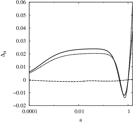
In Fig. 10 we plot the evolution of the relative deviation of the Hubble parameter from the $\Lambda$CDM as a function of $a$ for three best-fit models studied in this paper. The deviation $\Delta_{H}$ of the best-fit scaling model is very small, which reflects the fact that $w$ quickly approaches $-1$ after the early transition from the scaling regime. Meanwhile, in the best-fit thawing and tracker models, the relative deviations from the $\Lambda$CDM can reach the level of 2 %.

References

- [1] A. G. Riess et al. [Supernova Search Team Collaboration], Astron. J. 116, 1009 (1998); S. Perlmutter et al. [Supernova Cosmology Project Collaboration], Astrophys. J. 517, 565 (1999).
- [2] M. Hicken et al., Astrophys. J. 700, 1097 (2009).
- [3] D. N. Spergel et al. [WMAP Collaboration], Astrophys. J. Suppl. 148, 175 (2003).
- [4] E. Komatsu et al. [WMAP Collaboration], Astrophys. J. Suppl. 192, 18 (2011).
- [5] D. J. Eisenstein et al. [SDSS Collaboration], Astrophys. J. 633, 560 (2005).
- [6] W. J. Percival et al., Mon. Not. Roy. Astron. Soc. 401, 2148 (2010).
- [7] N. Suzuki et al., Astrophys. J. 746, 85 (2012).
- [8] S. Weinberg, Rev. Mod. Phys. 61, 1 (1989).
- [9] Y. Fujii, Phys. Rev. D 26, 2580 (1982); L. H. Ford, Phys. Rev. D 35, 2339 (1987); C. Wetterich, Nucl. Phys B. 302, 668 (1988); T. Chiba, N. Sugiyama and T. Nakamura, Mon. Not. Roy. Astron. Soc. 289, L5 (1997); P. G. Ferreira and M. Joyce, Phys. Rev. Lett. 79, 4740 (1997); R. R. Caldwell, R. Dave and P. J. Steinhardt, Phys. Rev. Lett. 80, 1582 (1998).
- [10] P. J. E. Peebles and B. Ratra, Astrophys. J. 325, L17 (1988); B. Ratra and J. Peebles, Phys. Rev D 37, 321 (1988).
- [11] T. Chiba, T. Okabe and M. Yamaguchi, Phys. Rev. D62, 023511 (2000); C. Armendariz-Picon, V. F. Mukhanov and P. J. Steinhardt, Phys. Rev. Lett. 85, 4438-4441 (2000).
- [12] V. Sahni and A. A. Starobinsky, Int. J. Mod. Phys. D 9, 373 (2000); S. M. Carroll, Living Rev. Rel. 4, 1 (2001); T. Padmanabhan, Phys. Rept. 380, 235 (2003); P. J. E. Peebles and B. Ratra, Rev. Mod. Phys. 75, 559 (2003); E. J. Copeland, M. Sami and S. Tsujikawa, Int. J. Mod. Phys. D 15, 1753 (2006); T. P. Sotiriou and V. Faraoni, Rev. Mod. Phys. 82, 451 (2010); A. De Felice and S. Tsujikawa, Living Rev. Rel. 13, 3 (2010); S. Tsujikawa, arXiv:1004.1493 [astro-ph.CO].
- [13] S. M. Carroll, Phys. Rev. Lett. 81, 3067 (1998).
- [14] C. F. Kolda and D. H. Lyth, Phys. Lett. B 458, 197 (1999).
- [15] P. Binetruy, Phys. Rev. D 60, 063502 (1999); P. Brax and J. Martin, Phys. Lett. B 468, 40 (1999); E. J. Copeland, N. J. Nunes and F. Rosati, Phys. Rev. D 62, 123503 (2000); P. K. Townsend, JHEP 0111, 042 (2001); S. Hellerman, N. Kaloper and L. Susskind, JHEP 0106, 003 (2001); R. Kallosh, A. D. Linde, S. Prokushkin and M. Shmakova, Phys. Rev. D 65, 105016 (2002); M. Gasperini, F. Piazza and G. Veneziano, Phys. Rev. D 65, 023508 (2002); A. J. Albrecht, C. P. Burgess, F. Ravndal and C. Skordis, Phys. Rev. D 65, 123507 (2002).
- [16] J. A. Frieman, C. T. Hill, A. Stebbins and I. Waga, Phys. Rev. Lett. 75, 2077 (1995).
- [17] Y. Nomura, T. Watari and T. Yanagida, Phys. Lett. B 484, 103 (2000); K. Choi, Phys. Rev. D 62, 043509 (2000); J. E. Kim and H. P. Nilles, Phys. Lett. B 553, 1 (2003); L. J. Hall, Y. Nomura and S. J. Oliver, Phys. Rev. Lett. 95, 141302 (2005); S. Panda, Y. Sumitomo and S. P. Trivedi, Phys. Rev. D 83, 083506 (2011).
- [18] R. R. Caldwell and E. V. Linder, Phys. Rev. Lett. 95, 141301 (2005).
- [19] I. Zlatev, L. M. Wang and P. J. Steinhardt, Phys. Rev. Lett. 82, 896 (1999); P. J. Steinhardt, L. -M. Wang and I. Zlatev, Phys. Rev. D 59, 123504 (1999).
- [20] E. J. Copeland, A. R. Liddle and D. Wands, Phys. Rev. D 57, 4686 (1998).
- [21] T. Barreiro, E. J. Copeland and N. J. Nunes, Phys. Rev. D 61, 127301 (2000).
- [22] A. Albrecht and C. Skordis, Phys. Rev. Lett. 84, 2076 (2000).
- [23] V. Sahni and L. -M. Wang, Phys. Rev. D 62, 103517 (2000).
- [24] T. D. Saini, S. Raychaudhury, V. Sahni and A. A. Starobinsky, Phys. Rev. Lett. 85, 1162 (2000); Z. Haiman, J. J. Mohr and G. P. Holder, Astrophys. J. 553, 545 (2000); C. Baccigalupi, A. Balbi, S. Matarrese, F. Perrotta and N. Vittorio, Phys. Rev. D 65, 063520 (2002); M. Yahiro, G. J. Mathews, K. Ichiki, T. Kajino and M. Orito, Phys. Rev. D 65, 063502 (2002); U. Alam, V. Sahni, T. D. Saini and A. A. Starobinsky, Mon. Not. Roy. Astron. Soc. 344, 1057 (2003); R. R. Caldwell and M. Doran, Phys. Rev. D 69, 103517 (2004); L. Perivolaropoulos, Phys. Rev. D 71, 063503 (2005) S. Nesseris and L. Perivolaropoulos, Phys. Rev. D 72, 123519 (2005); D. Huterer and H. V. Peiris, Phys. Rev. D 75, 083503 (2007); M. Sahlen, A. R. Liddle and D. Parkinson, Phys. Rev. D 75, 023502 (2007); S. Sen, A. A. Sen and M. Sami, Phys. Lett. B 686, 1 (2010); S. Thakur, A. Nautiyal, A. A. Sen and T. R. Seshadri, arXiv:1204.2617 [astro-ph.CO].
- [25] S. Dutta and R. J. Scherrer, Phys. Rev. D 78, 123525 (2008).
- [26] T. Chiba, Phys. Rev. D 79, 083517 (2009).
- [27] R. J. Scherrer and A. A. Sen, Phys. Rev. D 77, 083515 (2008).
- [28] T. Chiba, S. Dutta and R. J. Scherrer, Phys. Rev. D 80, 043517 (2009).
- [29] L. Anderson et al., arXiv:1203.6594 [astro-ph.CO].
- [30] N. G. Busca et al. [BOSS Collaboration], arXiv:1211.2616 [astro-ph.CO].
- [31] T. Clemson and A. R. Liddle, Mon. Not. Roy. Astron. Soc. 395, 1585 (2009).
- [32] G. Gupta, S. Majumdar and A. Sen, Mon. Not. Roy. Astron. Soc. 420, 1309 (2012).
- [33] T. Chiba, Phys. Rev. D 81, 023515 (2010).
- [34] C. R. Watson and R. J. Scherrer, Phys. Rev. D 68, 123524 (2003).
- [35] P. -Y. Wang, C. -W. Chen and P. Chen, JCAP 1202, 016 (2012).
- [36] A. de la Macorra and G. Piccinelli, Phys. Rev. D 61, 123503 (2000); S. C. C. Ng, N. J. Nunes and F. Rosati, Phys. Rev. D 64, 083510 (2001).
- [37] T. Chiba, Phys. Rev. D 66, 063514 (2002).
- [38] F. Piazza and S. Tsujikawa, JCAP 0407, 004 (2004); S. Tsujikawa and M. Sami, Phys. Lett. B 603, 113 (2004).
- [39] R. Bean, S. H. Hansen and A. Melchiorri, Phys. Rev. D 64, 103508 (2001).
- [40] E. V. Linder and D. Huterer, Phys. Rev. D 72, 043509 (2005).
- [41] B. A. Bassett, M. Kunz, J. Silk and C. Ungarelli, Mon. Not. Roy. Astron. Soc. 336, 1217 (2002); P. S. Corasaniti and E. J. Copeland, Phys. Rev. D 67, 063521 (2003); B. A. Bassett, P. S. Corasaniti and M. Kunz, Astrophys. J. 617, L1 (2004).
- [42] A. De Felice, S. Nesseris and S. Tsujikawa, JCAP 1205, 029 (2012).
- [43] J. R. Bond, G. Efstathiou and M. Tegmark, Mon. Not. Roy. Astron. Soc. 291, L33 (1997).
- [44] A. Kosowsky, M. Milosavljevic and R. Jimenez, Phys. Rev. D 66, 063007 (2002).
- [45] Y. Wang and P. Mukherjee, Phys. Rev. D 76, 103533 (2007).
- [46] W. Hu and N. Sugiyama, Astrophys. J. 471, 542 (1996).
- [47] D. J. Eisenstein and W. Hu, Astrophys. J. 496, 605 (1998).
- [48] C. Blake et al., Mon. Not. Roy. Astron. Soc. 415, 2892 (2011).
- [49] F. Beutler et al., Mon. Not. Roy. Astron. Soc. 416, 3017 (2011).
- [50] S. Dutta, E. N. Saridakis and R. J. Scherrer, Phys. Rev. D 79, 103005 (2009).
- [51] H. Akaike, IEEE Trans. Auto. Control, 19, 716 (1974); A. R. Liddle, Mon. Not. Roy. Astron. Soc. 351, L49 (2004).
- [52] N. Sugiura, Communications in Statistics, A7, 13-26 (1978).
- [53] W. Hu and I. Sawicki, Phys. Rev. D 76, 064004 (2007); L. Amendola and S. Tsujikawa, Phys. Lett. B 660, 125 (2008); H. Motohashi, A. A. Starobinsky and J. ’i. Yokoyama, Prog. Theor. Phys. 123, 887 (2010).
- [54] A. De Felice and S. Tsujikawa, Phys. Rev. Lett. 105, 111301 (2010); A. De Felice and S. Tsujikawa, JCAP 1202, 007 (2012).
- [55] V. A. Rubakov, Theor. Math. Phys. 149, 1651 (2006); M. Libanov, V. Rubakov, E. Papantonopoulos, M. Sami and S. Tsujikawa, JCAP 0708, 010 (2007).