Does a ‘stochastic’ background of gravitational waves exist in the pulsar timing band?
Abstract
We investigate the effects of gravitational waves (GWs) from a simulated population of binary super-massive black holes (SMBHs) on pulsar timing array datasets. We construct a distribution describing the binary SMBH population from an existing semi-analytic galaxy formation model. Using realizations of the binary SMBH population generated from this distribution, we simulate pulsar timing datasets with GW-induced variations. We find that the statistics of these variations do not correspond to an isotropic, stochastic GW background. The “Hellings & Downs” correlations between simulated datasets for different pulsars are recovered on average, though the scatter of the correlation estimates is greater than expected for an isotropic, stochastic GW background. These results are attributable to the fact that just a few GW sources dominate the GW-induced variations in every Fourier frequency bin of a 5-year dataset. Current constraints on the amplitude of the GW signal from binary SMBHs will be biased. Individual binary systems are likely to be detectable in 5-year pulsar timing array datasets where the noise is dominated by GW-induced variations. Searches for GWs in pulsar timing array data therefore need to account for the effects of individual sources of GWs.
Subject headings
black hole physics — galaxies: evolution — gravitational waves — methods: data analysisI. Introduction
Detecting and performing science with gravitational waves (GWs) is currently a major goal of experimental astrophysics. Pulsar timing arrays [18, 15, PTAs,] employ contemporaneous timing observations of millisecond radio pulsars in order to search for the effects of GWs perturbing the space-time metric along each pulsar-Earth line of sight. PTAs are complementary to other GW detection experiments, such as ground-based and space-based interferometers, in that they are sensitive to GWs in a different frequency band (currently nHz, i.e., periods of five years to a few months). In this frequency band, the most promising astrophysical sources of GWs are binary super-massive black holes (SMBHs).
SMBHs, with masses in the range to ,11 1 This mass range approximately corresponds to the current sample of SMBHs with dynamical mass measurements [30, cf.]. are of great importance to the evolution of galaxies. Feedback from active SMBHs is a key element in shaping properties of the observed galaxy population [16]. Models that trace the co-evolution of SMBHs and their host galaxies [11, e.g.,] postulate that SMBHs grow primarily through accretion and coalescence with other SMBHs during active phases triggered by galaxy mergers. Presumably, there exists a large population of binary SMBHs at various stages of coalescence in the cores of galaxies that have recently merged with other galaxies. The final stages of SMBH-SMBH coalescence are driven by losses of energy and angular momentum to GWs, primarily emitted in the PTA frequency band. Various works have predicted the average spectrum of the GW strain amplitude from the cosmic population of binary SMBHs [22, 46, 35]. Under the assumption that all binary systems are in circular orbits evolving only through GW emission, this spectrum takes the form [31]
| (1) |
where is the characteristic strain as a function of GW frequency, , at the Earth, and is the characteristic strain at a frequency of . The characteristic strain is the GW strain per logarithmic frequency interval, and is given by
| (2) |
where is the one-sided strain power spectral density (PSD).
The combined GW signal from binary SMBHs is widely assumed to form an isotropic, stochastic GW background. The value of is used to specify the amplitude of the background. The most recent predictions for the value of were made by Sesana et al. [35], who found a likely range of to . This range of predictions was derived by considering a variety of SMBH seeding, accretion and feedback scenarios, as well as uncertainties in the galaxy merger rate and in the SMBH mass function.
PTA projects are based on observations of periodic pulses of radio emission from pulsars using large radio telescopes. These observations lead to measurements of pulse times of arrival (ToAs) at the observatories. ToA measurements are typically conducted every few weeks over many years. Pulsar timing involves parameters of a physical model for the ToAs being fitted to the measured ToAs, with the differences between the observed ToAs and the model predictions being the timing residuals. ToAs can be modeled using combinations of deterministic and stochastic processes.
GWs incident on the Earth (and on the pulsars) cause shifts in the measured pulse frequencies of the pulsars [33, 10]. For a pulsar, indexed by , with intrinsic rotation frequency , consider a GW-induced shift, , to this frequency. This shift is a function both of time, , and the Earth-pulsar direction vector, . The resulting discrete time-series of GW-induced variations to the ToAs, (the subscript indicates that is sampled at times ), is given by [10]
| (3) |
For any GW signal, the expected values of zero-lag cross-correlations between the time-series for different pulsars can be specified. For any stochastic GW signal, the expected value of the normalized correlation for each pulsar pair is expressed in terms of the angular separations between the pulsars as [18, 23]
| (4) |
where , is the angular separation between pulsars and , and the Kroenecker delta, , is unity if , and zero otherwise. This function is known as the Hellings & Downs curve. An isolated source of GWs will give rise to correlations that are different from the the Hellings & Downs curve. Measurements of correlations between pulsar timing datasets that are attributable to the effects of GWs are necessary for the detection of GWs with PTAs [23, 48, 9].
The prospect of detecting or constraining the amplitude of a background of GWs from binary SMBHs has been the primary rationale for the development of the PTA concept. Various works have placed upper bounds on the value of for a background with the characteristic strain spectral form of Equation 1 [24, 43, 9]. The best published upper bound [43] finds that with 95% confidence. All analysis methods developed to study the combined GW signal from binary SMBHs with PTAs assume that the time-series for multiple pulsars can be described as a specific stochastic process. We describe the exact nature of this assumption in §2.
In this paper, we elucidate the statistical nature of the ToA variations induced by GWs from binary SMBHs. We accomplish this by modeling the GW signal from the predicted population of binary SMBHs, and by simulating realizations of corresponding to realizations of the GW signal. This study is critical to the validity of interpreting published upper limits on as representative of limits on the mean characteristic strain spectrum of GWs predicted to arise from binary SMBHs. Our results are also important for the optimization of GW detection techniques with PTAs. In §3, we outline our method of simulating pulsar timing datasets including GWs from the predicted population of binary SMBHs. Our analysis and results are presented in §4 and §5, and we discuss the interpretation and implications of our results in §6. We present our conclusions in §7.
Throughout this work, we assume a CDM concordance cosmology based on a combined analysis of the first-year WMAP data release [38] and the 2dF Galaxy Redshift Survey [5], with , , , and km s-1 Mpc-1. Although these parameter values have since been superseded by more recent observations, we adopt them in order to remain consistent with the model we use for the binary SMBH population [17]. A list of important symbols in this paper is shown in Table 1, along with the sections of the text in which they are introduced.
| Symbol | Section | Description |
|---|---|---|
| 1 | GW-induced ToA variation for pulsar at time . | |
| 1 | Expected zero-lag normalized cross-correlation between and time-series. | |
| 2 | Expected PSD of time-series. | |
| 2 | Periodogram estimator of at frequency . | |
| 3.1 | GW strain amplitude divided by frequency dependence. | |
| 3.1 | Binned distribution of binary SMBHs derived from realizations of the Millennium and Millennium-II coalescence lists. | |
| 3.1 | Average of 1000 realizations of . | |
| 3.1 | Analytic fit to . | |
| 3.2 | derived in terms of . | |
| 3.2 | Expected GW characteristic strain spectrum derived in terms of . | |
| 4 | 1 ns rms ToA variation at time . | |
| 4 | Sum of and . | |
| 4 | Expected PSD of time-series. | |
| 4 | Periodogram estimator of at frequency . | |
| 5 | Estimator of . |
II. The current model for ToA variations induced by gravitational waves from binary SMBHs
ToA variations induced by GWs from binary SMBHs () are commonly modeled among the PTA community as a wide-sense stationary random Gaussian process. This is based on the hypothesis that many GW sources forming a GW background contribute to the ToA variations, resulting in a statistical process governed by the central limit theorem. While the nature of the random Gaussian model for has been extensively described elsewhere [42, e.g.,], we summarize it here for completeness.
The key property of a random Gaussian process is that a linear combination of samples will have a joint normal distribution function. Different samples need not be statistically independent. The distribution of samples from a (zero-mean) random Gaussian process is characterized by the covariance matrix of the samples. Consider a vector, , containing samples of . That is,
| (5) |
Let be another vector defined similarly to , corresponding to a pulsar , containing simultaneously-obtained samples of . Under the random Gaussian assumption, the joint probability distribution of the samples in and , which we denote , is given by
| (6) |
Here, is an matrix containing the covariances between the samples of and ; that is, element of is given by the covariance between and . As the Gaussian process is wide-sense stationary, each element of depends only on the time difference between samples and for pulsar and respectively. Elements of are sampled from a covariance function, , between the GW-induced ToA variations for pulsars and . This covariance function is defined by the inverse Fourier transform of the one-sided PSD, , of GW-induced ToA variations for a given pulsar:
| (7) |
Here, denotes a complex Fourier transform, and is a time-lag. The PSDs of the GW-induced ToA variations for all pulsars are equivalent, and given by [24]
| (8) |
for a GW signal with the expected characteristic strain spectrum .
The above discussion applies equivalently if pulsar and pulsar are the same pulsar, or if they are different pulsars. The Hellings & Downs factor , defined in Equation 4, accounts for the correlation between GW-induced TOA variations for different pulsars. If has the form in Equation 1, we have . The GW-induced ToA variations for each pulsar will therefore be a “red” process. In this work, we only consider time-series with finite lengths .
We are interested in comparing a new model for with the random Gaussian model described in this section. To this end, we need to be able to simulate realizations of as a random Gaussian process. Multiple PTA groups test their data analysis algorithms by simulating realizations of using the GWbkgrd plugin [20] to the tempo2 pulsar timing package [19]. While this plugin does not explicitly generate random Gaussian realizations of by construction, we and others [43, 9] have checked that it approximates a random Gaussian process well.
In the plugin GWbkgrd, a number of GW oscillators, , are simulated between GW frequencies and , with the normally distributed and GW polarization amplitudes set to be purely real with zero mean, variance
| (9) |
and frequency probability distribution, , given by
| (10) |
ToA variations calculated for a given pulsar at different times corresponding to GWs from each of these oscillators are summed to produce a realization of the time-series. The frequency limits and are generally chosen respectively to be much less than the and much greater than the Nyquist frequency corresponding to the minimum sampling interval.
We make a distinction between the expected PSD of ToA variations induced by GWs from binary SMBHs, as defined in Equation 8, and estimates of this PSD based on realizations of the ToA variations. A commonly-used non-parametric, unbiased estimator of the PSD of a time-series is the periodogram [34]. The periodogram, , of is defined as
| (11) |
where DFT denotes a discrete Fourier transform. We adopt the following standard definition for the DFT of samples of :
| (12) |
where in this case. The DFT is evaluated for frequencies
| (13) |
where is the interval (assumed to be constant) between samples of . Throughout this work, we estimate the PSD, , of realizations of by evaluating .
III. Simulating pulsar ToA variations accounting for binary SMBH population characteristics
In this section, we describe a new method of simulating ToA variations caused by GWs from the predicted population of binary SMBHs. Various works have presented models for the cosmic demographics of binary SMBHs [13]. More recently, such efforts have been based on analytic prescriptions for baryon physics applied to dark matter halo merger tree catalogues from N-body simulations [17, hereafter G11]. In particular, the G11 prescriptions were applied to merger trees from both the Millennium [39] and the Millennium-II [2] simulations. The Millennium and Millennium-II simulations follow the evolution of dark matter structures, using the same physical prescriptions and number of particles. The Millennium-II simulation was however carried out in a comoving cubic volume with one-fifth the side length as that of the Millennium simulation, with the aim of resolving smaller-scale dark matter structures than the Millennium simulation.22 2 The Millennium-II simulation however does not reproduce larger-scale structures as well as the Millennium simulation. Together, these simulations resolve dark matter halos corresponding to the observed galaxy population, from dwarf galaxies to the largest-mass early-type galaxies.
The G11 model is the latest in a series [39, 7, 8] of semi-analytic prescriptions applied to the Millennium simulations. A host of observables of galaxies at low redshifts are reproduced, along with the redshift-evolution of the quasar population and star formation. Of most relevance here is that the model also traces the SMBH population, reproducing the SMBH-galaxy scaling relations in their slopes, normalization and scatters, as well as the inferred SMBH mass function [29].
We base our description of the binary SMBH population emitting GWs on the prediction for the SMBH-SMBH coalescence rate from the G11 model. We fit an analytic function to the distribution of binary SMBHs, and randomly draw GW sources from this distribution to produce realizations of the GW sky corresponding to binary SMBHs. We then add the effect of each GW source to simulated pulsar ToA datasets in order to analyze the GW-induced ToA variations.
This work is different from previous attempts to model the GW signal from binary SMBHs. Initial attempts [22, e.g.,] to predict the mean GW characteristic strain spectrum from binary SMBHs used empirical determinations of the galaxy merger rate and the SMBH mass function. Wyithe & Loeb [46] predicted the GW spectrum by analytically following the dark matter halo merger hierarchy in an extended Press-Schechter framework, and by deriving the SMBH coalescence rate by relating the SMBH masses to the halo circular velocities. Sesana et al. [35] considered the possible range of predictions of the characteristic strain spectrum, using Monte Carlo realizations of dark matter halo merger trees and various prescriptions for SMBH growth.
The key difference between the present work and previous calculations of the GW signal from binary SMBHs is that we are chiefly concerned with the statistics of . Our approach to modeling the binary SMBH population is similar to Sesana et al. [36] in our use of mock galaxy catalogues derived from analytic prescriptions applied to the Millennium simulations. However, whereas Sesana et al. [36] modeled the SMBH population by using empirical SMBH-galaxy scaling relations combined with (earlier) mock catalogues, we utilize SMBHs modeled by G11 in a self-consistent framework which reproduces the relevant observables.
III.1. Modeling the distribution of binary SMBHs
As in the previous works discussed above, we consider all binary SMBHs to be in circular orbits, and use expressions for the resulting GW emission presented by Thorne [40]. We briefly discuss the assumption of circular orbits in §6.3. The strain amplitude, , at frequency of GWs from a circular binary, averaged over all orientations and polarizations, is given by:
| (14) |
where is the universal gravitational constant, is the chirp mass of the binary, is the vacuum speed of light, is the redshift, and is the comoving distance to the binary. The evolution of the received GW frequency with observed time, , is determined by
| (15) |
The rest-frame binary orbital frequency is given by . We assume, after Hughes [21], that the maximum received frequency, , is attained at a binary separation of three Schwarzschild radii, corresponding to the last stable orbit:
| (16) |
assuming a mass ratio of unity.
The mock galaxy catalogues resulting from the G11 model are available online33 3 http://www.mpa-garching.mpg.de/millennium/ [27]. The halo merger trees from the Millennium and Millennium-II simulations were evaluated at 60 logarithmically-spaced redshift “snapshots” between and . We obtained the lists of SMBH-SMBH coalescence events within the comoving volume of each simulation by querying the online database. Redshifts at the (non-logarithmic) midpoints between the redshift snapshots were assigned to each event. We used these lists to fill bins of a distribution, , of the number, , of observable binary SMBHs per unit comoving volume per solid angle on the sky, given by
| (17) |
where
| (18) |
and is the sky-integrated comoving volume shell between redshifts and . Also, , and the derivative was obtained from Equation 15. is the predicted distribution of binary SMBHs in (which corresponds to the frequency-independent GW “power”, or squared strain amplitude) and the observed GW frequency.
For chirp masses below , the limited capability of the Millennium simulation to resolve low-mass halos caused an under-prediction of the chirp mass function as compared to the Millennium-II simulation. In order to ensure a complete chirp mass function, we included binary SMBHs with from the Millennium list of coalescence events, and binaries with from the Millennium-II list.
Some degrees of randomization in the coalescence lists were possible. First, in cases where more than two SMBHs coalesced to form a single SMBH between redshift snapshots, the merger order was not specified. In these instances we randomized over merger order. Second, a spherical comoving volume shell between any pair of redshifts less than could be contained within the simulation volume. Some Millennium redshift snapshots exist at , and the comoving volume shells between redshifts corresponding to these snapshots enclose some SMBH-SMBH coalescence events in the G11 model. An observer located at the center of the Millennium simulation volume would observe only a fraction of the total list of events in the G11 model at , and an observer located elsewhere in the volume would observe a different selection of events. This is not the case for the Millennium-II simulation, where the volume was too small to enclose any comoving volume shells between redshift snapshots. For each realization of the Millennium (but not the Millennium-II) coalescence list, we therefore specified randomly-placed spherical shells within the simulation box to select binary SMBHs at these redshifts. For coalescence events at , the corresponding comoving volume shells between redshift snapshots were smaller than the Millennium simulation volume, though not enclosed by it. For these coalescence events, we randomly included binaries in the Millennium coalescence list according to probabilities given by the ratios between the volumes of the comoving shells and the Millennium simulation volume. We used 1000 realizations of the Millennium and Millennium-II coalescence lists to form realizations of the binary SMBH distribution .
In generating realizations of the distribution , we assumed that every SMBH-SMBH coalescence event in the G11 model catalogues was the result of a binary SMBH system that had decayed through GW emission. The G11 model included the assumption that, upon the merger of two galaxies with central SMBHs, the SMBHs coalesced in every case, before accretion onto the newly-formed SMBH.44 4 There are various mechanisms by which extreme mass ratio binary SMBH systems and triple or higher-order systems can avoid coalescence [45, e.g.,]. We note that SMBHs with masses as low as were present in the G11 model catalogues, but were not included in the distributions. We verified that relaxing the lower cutoff on the SMBH masses in the distributions from to did not significantly modify the total signal.
The 1000 realizations of were averaged to form a distribution . We fitted with an analytic function which could be used to generate random realizations of the observable binary SMBH population. We did not use realizations of as realizations of the binary SMBH population because the -distributions were binned for computational purposes. A four-parameter function,
| (19) |
with free parameters , , and , was found to fit well. We performed the fit on the logarithm of the data to approximate linearity in the fitting procedure. The best-fit parameters are given in Table 2. The frequency-exponent was held fixed at , as predicted by Equations 15 and 17.
III.2. Realizations of pulsar ToAs with GW-induced variations
For a set of binary SMBHs drawn from the distribution , we simulated a corresponding time-series by summing the contributions from each individual binary. Details of the method used to calculate these contributions are presented in Hobbs et al. [20]. For each binary, we randomized over the right ascension and declination, the orbital inclination angle, the orientation of the line of nodes, and the orbital phase angle at the line of nodes. A new publicly-available tempo2 plugin, “addAllSMBHBs”, was written to perform this simulation.
For most of the present work, we did not use tempo2 to fit timing model parameters. Instead, we made use of the tools available for spectral analysis of timing residuals. In our simulations, the “timing residuals” corresponded exactly to given the absence of timing model fitting.
We consider it important to emphasize the distinction between the time-series and the timing residuals resulting from analyses of observed ToA datasets. Consider a set of observed ToAs that exactly match a particular timing model, except for the addition of GW-induced variations (a time-series). Given that an observer does not actually possess any prior knowledge of the timing model parameters, the observer will fit the model parameters to the ToAs. The resulting timing residuals will not be equivalent to . This is because the variations in the ToAs can alter the apparent pulsar timing parameters. For example, the presence of a time-series consisting of a sinusoidal signal with a period of one year will alter the apparent pulsar position.
In order to investigate the statistics of given our model for the binary SMBH population, we first used tempo2 to generate 500 ToAs spanning 5 years exactly corresponding to the PSR J04374715 timing model [28]. We then added realizations of the time-series evaluated at the observed ToAs to these datasets, that is, with yr and yr. The pulsar distance was set to 1 kpc, and the position was held fixed for all simulations. As the binary SMBHs used to produce realizations of had randomized positions and orientations, allowing the pulsar position to vary between realizations would not alter our results. The results presented in this paper are not dependent on the timing model used or on the pulsar distance from the Earth. We also added Gaussian white noise variations with 1 ns rms to the ToAs. This white noise component is much smaller than is usually observed in ToA datasets, but was necessary to smooth over machine precision errors.
| Parameter | Value |
|---|---|
| 4.878 | |
| 1.72249 | |
| 0.3473 |
We included GW sources between Hz and Hz in our simulations of . The lower frequency cutoff was chosen to be less than one fifth of . The upper frequency cutoff was chosen to be greater than . We assumed, after previous works, that all GW sources between these frequency cutoffs are non-evolving over a 5-year timespan, i.e., they do not evolve in frequency by more than (5 years)-1. The upper bound on the -values of sources, , was set by the last stable orbit of binary SMBHs. We identified this bound by fitting a power law to the high- edge of the distribution. The lower bound on , , was set by the lowest non-zero -value in . This value corresponds to a binary SMBH containing two components at . The distribution included more than GW sources within this domain; the vast computational cost involved makes it impossible to simulate with this many sources. Fortunately, the shape of the distribution was such that, at a given frequency, the highest- sources contributed most to (we return to this point below), defined in terms of (using Equation 8) as:
| (20) |
The average characteristic strain spectrum derived from is
| (21) |
We found a function, , such that
| (22) |
Thus, the GW sources in the domain contribute, on average, 90% of at every frequency. Between Hz and Hz, this amounted to sources. We refer to this domain as the “90% domain”. The 90% domain, along with , and , is shown in Figure 1.
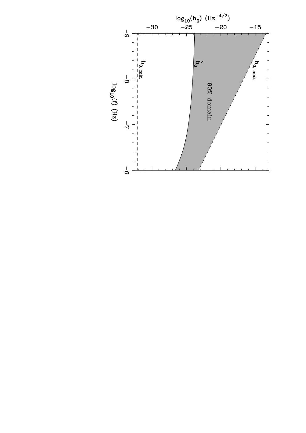
We approximated the total number of sources () in the domain between and and between Hz and Hz as constant. For a given realization of , the actual number of sources in the 90% domain is governed by binomial statistics. We therefore drew a (binomial-)random number of sources from the 90% domain, and added contributions from each of them to each realization of . We assumed that the sources remaining in the distribution with , contributing on average 10% to at every frequency, resulted in a stochastic contribution to governed by the central limit theorem. We therefore simulated them as described in §2 using the method of simulating ToA variations corresponding to a GW background implemented in the tempo2 plugin GWbkgrd. We simulated sources between Hz and Hz using the tempo2 method, with the characteristic strain spectrum given by . For each realization of , we added contributions from the GW sources drawn from the 90% domain of the distribution, and from the GW sources corresponding to the remaining (on average) 10% of drawn using the tempo2 method. Shifts in the measured pulse frequencies caused by metric perturbations at both the Earth and the pulsar (i.e., the “Earth term” and the “pulsar term”) were included in our simulations.
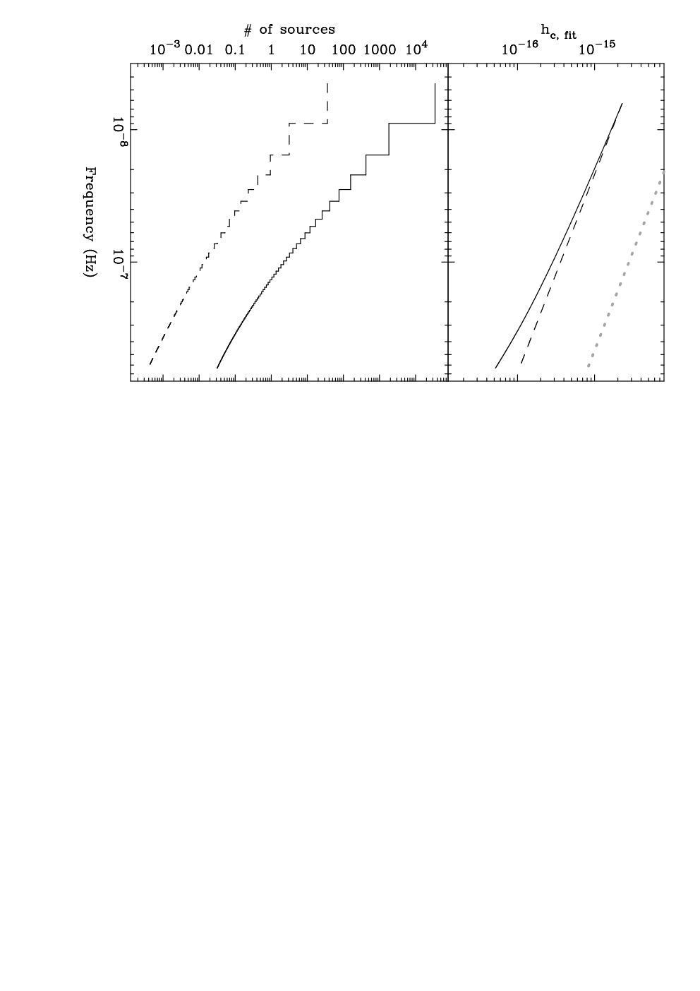
The top panel of Figure 2 shows in the spectral bins. We also show a characteristic strain spectrum of the form in Equation 1 with . This value of can be taken to be the prediction from the G11 model, as it corresponds to the characteristic strain in the lowest () spectral bin of a 5-year dataset. This particular curvature in the curve, also predicted by Wyithe & Loeb [46], is caused by the frequency-dependence of , which represents the bound beyond which binary SMBHs have crossed the last stable orbit. This curvature is caused by different processes from the curvature reported by Sesana et al. [35]. We show the mean characteristic strain spectrum for GWs from all binary SMBHs in the predicted distribution . Sesana et al. [35] fitted a broken power-law to realizations of the characteristic strain spectrum, accounting for various randomizations over the source population. In particular, Sesana et al. [35] randomized over the existence of “fractional” sources in every frequency bin of a fiducial dataset, and also excluded the strongest single source in every frequency bin in an attempt to isolate the background signal. The smaller number of sources per unit frequency at higher GW frequencies, combined with the greater contributions to the signal from the strongest single sources in frequency bins at higher frequencies, both resulted in the curved characteristic strain spectra presented by Sesana et al. [35].
The bottom panel of Figure 2 shows the mean numbers of highest- sources that contribute 90% and 50% of in these frequency bins. A small number of sources contribute a large fraction of at every frequency. In the frequency bin, the highest- sources contribute on average 90% of , and only 30 sources on average contribute 50% of . At frequencies Hz, the strongest source, on average, contributes more than 90% of in each frequency bin. This is a consequence of the shallow power-law nature of the -distribution of the GW sources in the distribution.
In this work, we compare the Millennium-based simulations of with simulations of created using the tempo2 method described in §2. To this end, we simulated ToAs as before, but added realizations of corresponding to oscillators simulated using the tempo2 plugin GWbkgrd. These oscillators were simulated as described in §2 with a mean characteristic strain spectrum given by . We refer to this latter method of simulating as Case H09, after Hobbs et al. [20]. Simulations of using GW sources drawn from will be referred to as Case R12 after the present work.
IV. Fourier-spectral analysis, and results
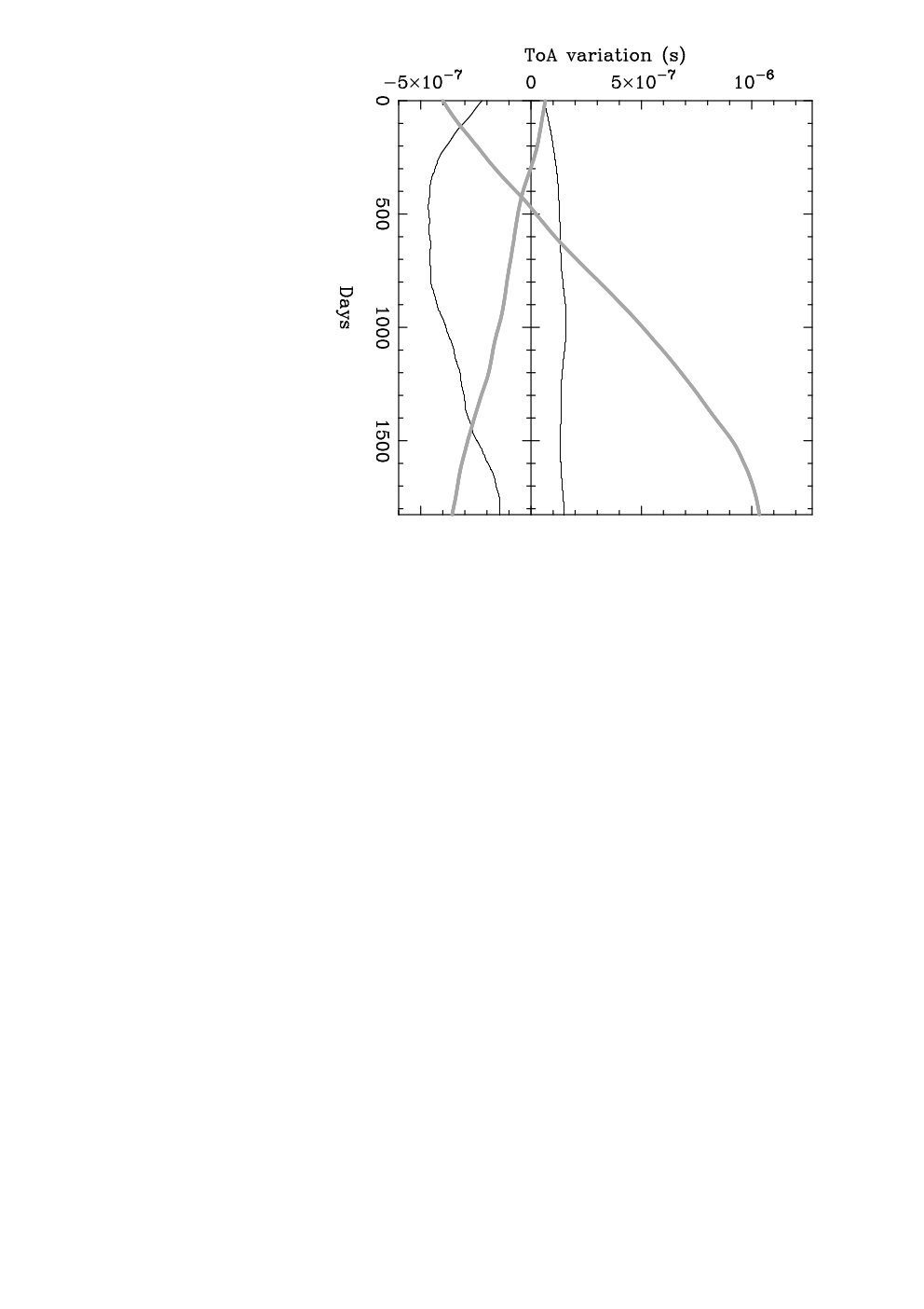
In this section, we consider the differences between the cases in the distributions of the periodograms, , evaluated for realizations of for a single pulsar. This is motivated by the results in Figure 2, in particular that the number of GW sources per spectral bin that contribute 90% of varies significantly with frequency. The Case R12 simulations are intended to more accurately represent the effects of GWs from binary SMBHs on ToA datasets than the Case H09 simulations. Example realizations of 5-year time-series in both cases are shown in Figure 3. The time-series appear quite similar: realizations in both cases are dominated by low-frequency components. Values of up to 1 s are also present in one realization.
Instead of directly measuring , the added white noise component in the simulated ToAs required us to analyze the periodograms of a time-series, , given by
| (23) |
where is a time-series of Gaussian white 1 ns rms ToA variations as discussed above. The PSD of , , is significantly red, with a spectral index of (see Equations 1, 20), and is expected to dominate the PSD of at low frequencies. We used the generalized least-squares algorithm described in Coles et al. [4] to measure the periodograms, of realizations of . This method requires knowledge of the auto-covariance function of , which we obtained as in Equation 7 using the inverse DFT of the known PSD of , , given by
| (24) |
In the following, we consider the distributions of in the lower spectral bins, where , to be approximately equivalent to the distributions of .
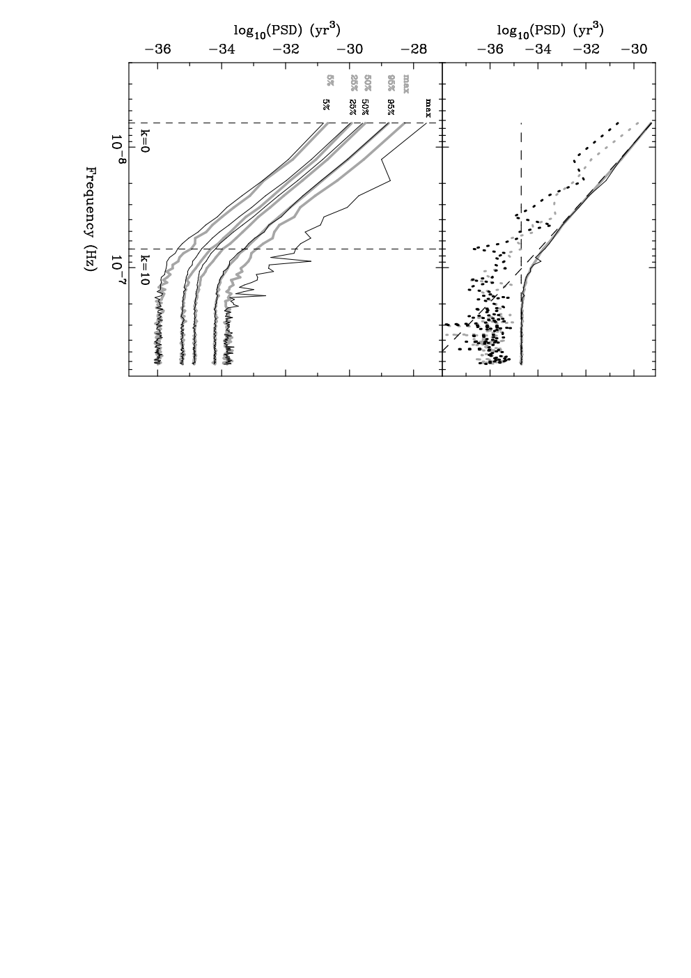
We produced 1000 realizations of in Case R12 and in Case H09, and measured for each realization. In the top panel of Figure 4, we show the averages of measured from each of the Case R12 and Case H09 realizations, along with the expected PSDs of and . Arbitrarily chosen single realizations of in each case are also shown. The means of the periodograms in both cases are clearly the same, and equivalent to the predicted PSD, , given in Equation 24. Though this is as expected, it is both a check of the simulations of , and a demonstration of the ability of our PSD estimation method to measure steep red spectra without bias.
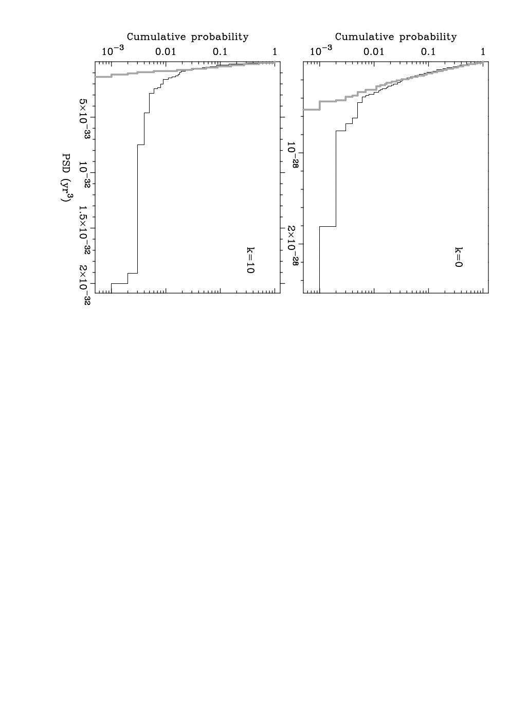
In contrast, the distributions of in the frequency bins where are different between the cases. The single realizations of in each case shown in the top panel of Figure 4 begin to hint at these differences. In most spectral bins, the Case R12 periodogram is below the Case H09 periodogram. That this is a genuine trend is confirmed in the bottom panel of Figure 4. Here, we depict various “percentile” periodograms of the distributions of in each of Case R12 and Case H09. The percentile periodograms may be interpreted as contours of equivalent percentiles of the periodogram distributions in different spectral bins. For example, the “50%” percentile periodogram links the 50th percentile points of the distributions of periodogram values in each spectral bin. Below the 95th percentile, all Case R12 percentile periodograms lie below Case H09 percentile periodograms. This implies that in most spectral bins, most measurements of a periodogram in Case R12 will, like the individual ones shown in the top panel of Figure 4, be below most Case H09 periodograms. However, the 95th percentile periodograms are essentially equivalent, and the maximum value Case R12 periodogram is well above the maximum value Case H09 periodogram. These implied “tails” at high values in the Case R12 periodogram distributions in each spectral bin are highlighted in Figure 5, which depicts the distributions of the in the spectral bins indicated by the vertical lines in the bottom panel of Figure 4. The distributions are shown as the fractions of Case R12 and Case H09 periodograms at or above a given value.
Figure 5 also shows that the Case R12 periodogram distribution in the spectral bin has a longer tail relative to the Case H09 distribution, as compared to the spectral bin. This effect is also evident in the bottom panel of Figure 4, in that the fractional differences between the percentile periodograms are greater at the upper end of the GW-dominated frequency regime. This is consistent with the number of GW sources per spectral bin included in the Case R12 simulations going down with increasing frequency, as shown in Figure 2.
In summary, approximating with as discussed above, we find that:
- •
In most spectral bins, most realizations of in Case R12 will be below most realizations of in Case H09.
- •
The maximum possible values of in Case R12 will be higher than the maximum possible values of in Case H09.
V. Estimates of correlations between GW-induced ToA variation time-series
Hellings & Downs [18] showed that the average values of correlations between for different pulsars, for a stochastic GW signal, will always be given by the Hellings & Downs curve (Equation 4). The distributions of individual estimates of these correlations, much like the distributions of the PSD estimator considered above, will however depend on the nature of the GW signal. Here, we characterize the distributions of estimates of these correlations for multiple pulsar pairs in each case discussed above. We simulated 100 realizations of each of Case H09 and Case R12 ToAs as described in §3.2 for pulsars at the positions of each of the 20 pulsars timed by the Parkes PTA, using the timing models specific to each pulsar [28]. For each realization, the same set of GW sources was used to simulate GW-induced ToA variations for each pulsar. The pulsar distances were set arbitrarily between 1 kpc and 20 kpc.
We estimated the correlations between time-series and , , for each pulsar pair in each realization of Case R12 and Case H09 ToAs. No autocorrelations were estimated. A frequency-domain estimation technique, based on the method of Yardley et al. [48], was used. This technique will be detailed elsewhere (Hobbs et al., in preparation). We refer to our estimates of as . These estimates were performed using time-series, rather than time-series (see Equation 23), and the estimation technique was optimized using the expected PSD of given in Equation 24. The technique removes best-fit linear and quadratic terms from each time-series using the standard tempo2 least-squares fitting algorithm. This mimics the effect of fitting pulse frequency and frequency-derivative terms to the simulated ToAs and then analyzing the timing residuals.
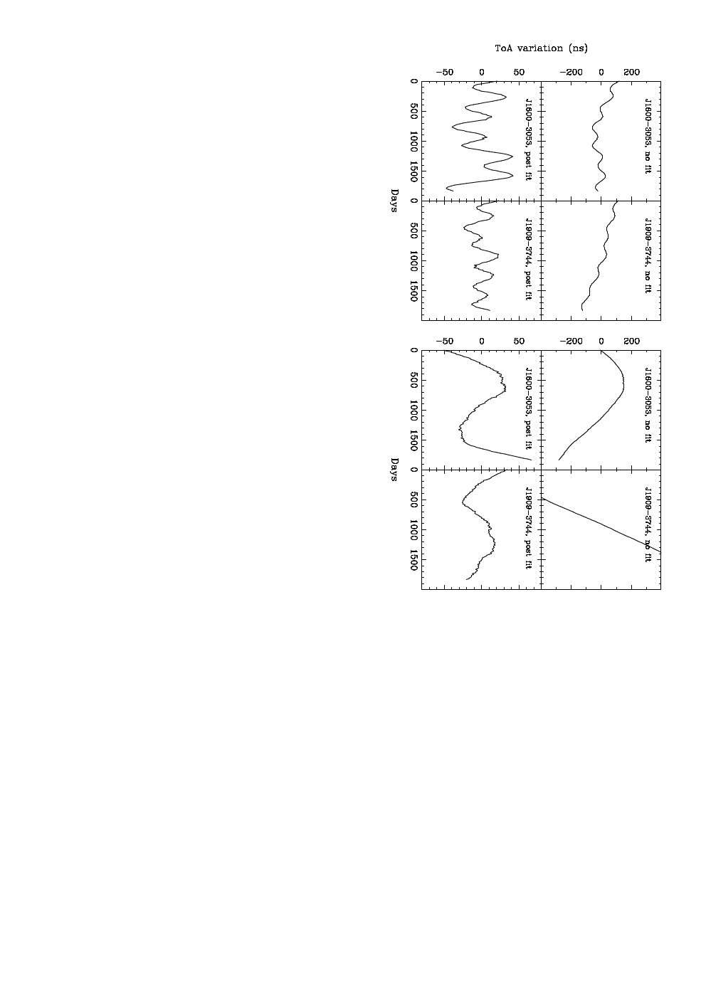
Following the removal of linear and quadratic terms from one of the 100 Case R12 realizations of , a single GW source was found to dominate the residual time-series. We show the corresponding time-series for two of the 20 simulated pulsars for this realization in Figure 6. The left panel of this Figure shows the large sinusoidal oscillations induced by the source, and the right panel shows example Case R12 realizations of that are not dominated by an individual source. It is possible that an individual GW source with a period greater than the 5-year dataspan could dominate the realizations of in the right-hand panel of Figure 6. The ToA variations induced by such a source would however be absorbed in the removal of the linear and quadratic terms from the time-series.
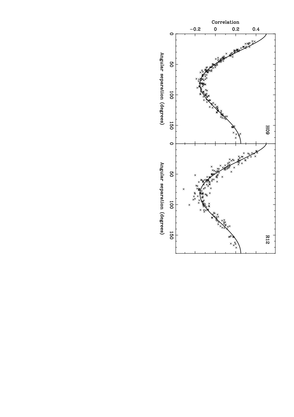
We averaged all measurements of for each pulsar pair from the Case R12 realizations, besides the one clearly dominated by an individual source. The realization dominated by an individual source added a large amount of scatter to the average Case R12 correlations, and was left out of the average to enable a better comparison between the cases. We also averaged the Case H09 measurements of for each pair in 99 arbitrarily-chosen realizations. The average measurements of are shown for both cases in Figure 7. The functional form of the Hellings & Downs curve is recovered in both Case R12 and Case H09. However, the Case R12 estimates are significantly more scattered about the expected values of the correlations than the Case H09 estimates.
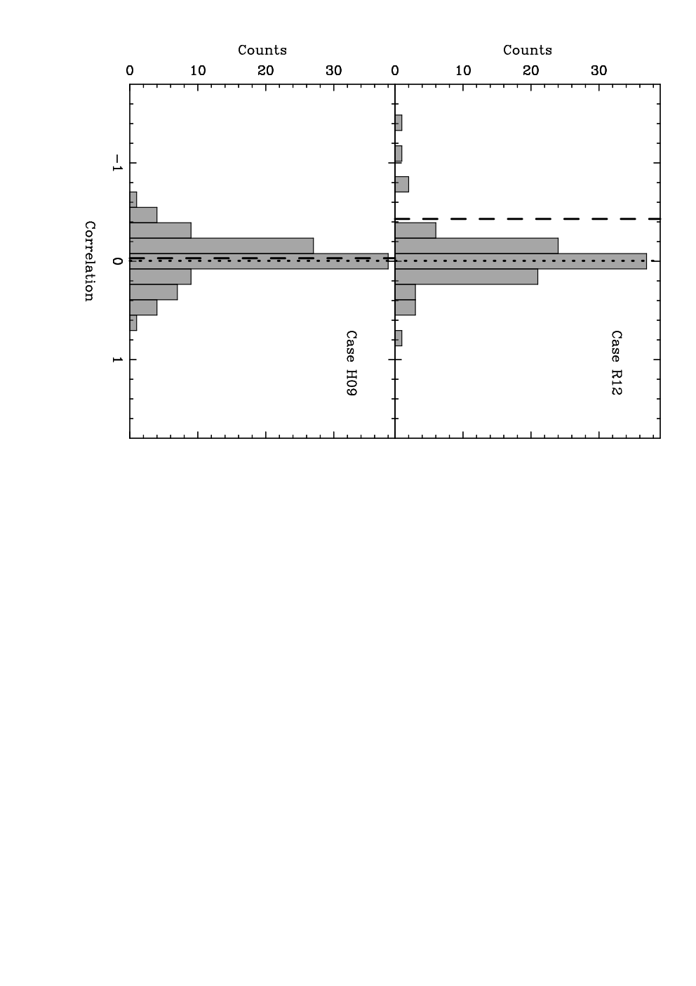
The increased scatter in the Case R12 correlations with respect to the Case H09 correlations in Figure 7 is caused by outlying estimates in only a few realizations of ToAs. This is shown in Figure 8, where we display the histograms of the measurements between simulated ToA datasets for PSR J04374715 and PSR J06130200 in each case. Correlation estimates were possible because we normalized the estimated covariances between time-series using the expected cross-PSD between the time-series. While most measurements in both cases are concentrated about the expected value of , a few Case R12 measurements are significantly displaced. This is consistent with the results of §4. We also stress that the large scatter of the estimator common to both cases is expected, and intrinsic to the GW signal.
VI. Discussion
We have shown that the ToA variations induced by GWs from the predicted binary SMBH population are not consistent with the model described in §2. The random Gaussian model for described in §2 and approximated in Case H09 is reasonable given that a large number of GW sources are expected to contribute to the GW-induced ToA variations. That is, the values of at all times are the sums of many random variables. An argument based on the classical central limit theorem would suggest that would then be Gaussian random at every time . It is apparent, however, that such a central limit theorem-based argument does not apply to the Case R12 realizations of . This is because of the nature of the GW sources contributing to in Case R12.
In Case R12, a few sources contribute most of the PSD of at every frequency, as shown in Figure 2. These sources are rare, because they are found at the high- tail of the source distribution. The estimators we consider in this work, and , are dominated in Case R12 by a few GW sources that need not occur in every realization of the time-series. This is why the distributions of these estimators are different between the cases. The quantities that we estimate, and , are used to define the covariance matrix of the GW-induced ToA variations (see Equation 7). We have therefore shown that the ToA variations induced by GWs from binary SMBHs are dominated by the effects of a few strong, rare sources and cannot be accurately modeled using the random Gaussian process discussed in §2.
VI.1. Implications of our results for experiments focused on a GW background
Current PTA data analysis techniques use assumptions about the statistics of to attempt to estimate or constrain the amplitude of the characteristic strain spectrum of GWs from binary SMBHs. We consider the implications of our results for a selection of techniques in turn. We assume, in this discussion, that our results for the statistics of GW-induced ToA variations would apply even if the normalization of the GW characteristic strain spectrum , which we refer to as the GW amplitude,55 5 We make a distinction between this amplitude and the parameter introduced in Equation 1, because does not have exactly the same form as given in Equation 1. were scaled up or down. Such a scaling could occur, for example, under different scenarios for whether coalescing SMBHs accrete gas before or after coalescence [35].
We summarize a few key techniques here:
- •
Jenet et al. [23] describe a statistic which measures the degree of correlation between estimates of from ToA data, and the expected functional form of . The expected detection significance, which is estimated under the assumption that the GW-induced ToA variations are Gaussian random, saturates at high values of the GW amplitude once the variance of the statistic is dominated by the stochasticity of the GW signal (see our Figure 8 and related discussion).
- •
Jenet et al. [24] constrain the amplitude of the GW characteristic strain spectrum from binary SMBHs by estimating the maximum possible GW signal present in measured data, under the assumption that the data could be modeled using a white noise process and GW-induced ToA variations. A statistic that estimates the GW background amplitude from individual pulsars was measured, and compared to the simulated distributions of the statistic for different GW amplitudes. The simulated statistic distributions were created from simulated ToA datasets with GW-induced ToA variations included using the tempo2 plugin GWbkgrd.
- •
van Haasteren et al. [42] present a Bayesian parameter estimation method for the GW characteristic strain spectral amplitude.66 6 Though their method also estimates the spectral index of the GW characteristic strain spectrum, we assume marginalization over this parameter in our discussion here. van Haasteren et al. [43] used this method to constrain the GW amplitude. This method requires an evaluation of the likelihood of the parameters used to model the ToA datasets, which include the GW amplitude. The likelihood is the probability distribution of the data given the model parameters. The GW amplitude is used to calculate the covariance matrix, , between the GW-induced ToA variations for pulsars and (see Equations 7, 8). This covariance matrix in turn is used to define the PTA likelihood, assuming that the GW-induced ToA variations can be modeled as a random Gaussian process.
- •
Demorest et al. [9] use a PTA likelihood similar to the work of van Haasteren et al. [42] to constrain the GW amplitude by evaluating the distribution of a maximum likelihood estimator for the amplitude. They also use a method similar in concept to Jenet et al. [23] to attempt to detect the GW signal from binary SMBHs.
First, the non-Gaussianity of the GW-induced ToA variations means that the estimate of the intrinsic GW-induced variance of the Jenet et al. [23] statistic will be incorrect. This will affect estimates of the detection significance, particularly in the “strong signal regime”, where the effects of GWs in the ToAs are large compared to all other noise processes. Second, the limit on the GW amplitude placed by Jenet et al. [24] will be biased. The Jenet et al. [24] limit was placed by finding the GW amplitude for which 95% of simulated statistic values were above the measured value. The distribution of their statistic derived using our simulations would be different. Ruling out a GW amplitude using the Jenet et al. [24] technique does not necessarily rule out a GW signal corresponding to our simulations with the same confidence. Finally, our results indicate that the likelihoods evaluated by van Haasteren et al. [42] and Demorest et al. [9] will also be biased, leading to a similar effect on GW amplitude constraints made using their methods. A definitive statement on the magnitude of the consequences of our simulations for current constraints on the GW amplitude cannot be made, however, without fully considering the various PTA data analysis methods.
VI.2. Single GW source detection prospects
We have established that in every frequency bin of the 5-year datasets we consider, a few strong GW sources dominate the PSD of . This means that we cannot consider the expected GW signal from binary SMBHs to form a background.77 7 This result is analogous to the case of the extragalactic background light [12], where the summed electromagnetic radiation from AGN and star-forming galaxies is dominated by strong individual sources, behind which myriad further objects combine to form an apparently isotropic background too uniform to be resolved by current telescopes. We briefly consider the prospects for there being single sources of GWs that are detectable by PTAs. Various methods of detecting and characterising individual continuous sources of GWs with PTAs have recently been presented [47, 3, 6, 26, 1, 14]. There are, however, few predictions for the expected numbers of detectable sources. Sesana et al. [36] analysed similar binary SMBH population models to those considered here to suggest that a 5-year ToA dataset would include 510 single GW sources above the mean “stochastic background” level, mainly at GW frequencies greater than Hz. Their definition of a resolvable source as one which has a (mean) strain amplitude that is greater than the mean background level is conservative. This is because a PTA is capable of spatial, as well as frequency resolution. The background contribution per spatial resolution element of a PTA will be less than the all-sky background level, resulting in a higher source amplitude to background ratio for a bright source located in the resolution element.
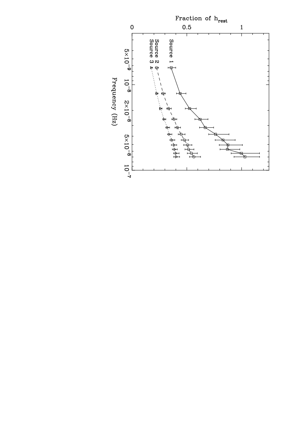
The exact number of resolvable GW sources given a GW background level for PTAs depends on the particular search method. For example, Boyle & Pen [3] suggest that a PTA composed of pulsars could resolve up to sources per frequency bin. In Figure 9, we present a simple indication of the expected amplitudes of strong individual sources in the spectral bins of our fiducial 5-year dataset. Using 300 Case R12 realizations of the GW source population, we found the mean strain amplitudes in each spectral bin of the strongest three GW sources. We express these amplitudes as multiples of the mean summed strain amplitude, , of the remaining sources. The errors in the values were not included in the error bars as they were very small.
If we consider the sources besides the strongest three in a spectral bin to form a ‘‘background’’,88 8 This is by no means a rigorous definition of a background relative to the number of sources. The exact definition is dependent on the single source search method and the characteristics of the PTA. it is clear that, for spectral bins with , three sources, on average, produce the same total strain amplitude as the remaining sources. Even for the spectral bin, three sources are expected to produce more than half the total strain amplitude of the remaining sources. Indeed, the strongest source in the spectral bin has an average strain amplitude that is , which implies that a PTA which can resolve out two-thirds of the sky will detect equal contributions from the source and from the background.
Blind searches for single GW sources with PTAs are therefore important. PTA data analysis methods that attempt to detect an isotropic component will not optimally recover the entirety of the GW signal from binary SMBHs, and could perhaps miss a large component of the signal for some realizations of the GW source population. A careful consideration of the efficacy of GW background detection methods as compared to search methods for single sources, given the predicted source characteristics, is required.
VI.3. Limitations of our approach to modelling the GW signal from binary SMBHs
A shortcoming of our approach towards modeling , and indeed of all predictions for the GW signal from binary SMBHs to date, is the assumption of circular orbits for all binaries. Recent work [37, 32, 25, e.g.,] suggests that binary SMBHs emitting GWs in the PTA frequency regime will have highly eccentric orbits. The candidate binary SMBH OJ 287 [41, e.g.,] is in fact modeled with an orbital eccentricity of 0.7. The GW waveform of an eccentric binary radiating in the PTA band spans many frequencies, and does not follow the frequency-time relation of Equation 15, or the dependence of the GW strain amplitude on frequency of Equation 14. Therefore, if most binary SMBHs radiating in the PTA band are eccentric, the predicted mean spectral slope of the characteristic strain spectrum (Equation 1) will change. We will also need to account for the binary eccentricity distribution in our predictions of the statistics of GW-induced ToA variations. Other effects that require further investigation are the effects of gas and stars on binaries. We do not include these effects in our model because the understanding of their combined contributions towards specifying the binary SMBH population is not sufficiently advanced.
VII. Conclusions
We have used a sophisticated model for galaxy evolution [17] to predict the distribution of binary SMBHs radiating GWs in the PTA frequency band. By drawing lists of GW sources from this distribution, we simulate the effects of GWs from binary SMBHs on 5-year pulsar ToA datasets. We compare these simulations (Case R12) with simulated pulsar datasets containing the effects of an equivalent-amplitude GW signal modeled as a random Gaussian process (Case H09). We estimate the PSDs of the simulated GW-induced ToA variation time-series, and the correlations between these time-series for different pulsars. We find that the distributions of the PSD estimators of the realizations of the GW-induced ToA variations are different between the cases in every frequency bin, although the mean estimated PSDs are the same in each case. While in Case R12 the estimated PSDs are concentrated at lower values than in Case H09, the Case R12 estimations extend to higher PSD values than the Case H09 estimations. We also find that the functional form of the Hellings & Downs curve is recovered on average in both cases. The correlations between the GW-induced ToA variation time-series for different pulsars in Case R12 are, however, significantly more scattered about the expected values than in Case H09. We interpret our results in terms of the influence of strong individual GW sources on the ToAs in Case R12.
We conclude the following:
- 1.
The effects of GWs from binary SMBHs on pulsar ToAs cannot be accurately modeled using existing methods, i.e, as a random Gaussian process. This is because a few GW sources dominate the PSD of the GW-induced ToA variations at all frequencies, with reducing numbers of sources contributing equivalent PSD fractions in higher frequency bins.
- 2.
Our results directly affect existing PTA data analysis methods aimed at detecting or estimating the parameters of the GW signal from binary SMBHs. The projected detection significance will be biased.
- 3.
The prospects for single GW source detection are strong. Individual sources could potentially be resolved in all GW-dominated frequency bins of a 5-year dataset.
We emphasize that future searches for GW signals from binary SMBHs in pulsar datasets need to be sensitive to both individual sources as well as a GW background.
References
- [1] Babak, S., & Sesana, A. 2012, Phys. Rev. D, 85, 044034
- [2] Boylan-Kolchin, M., Springel, V., White, S. D. M., Jenkins, A., & Lemson, G. 2009, MNRAS, 398, 1150
- [3] Boyle, L., & Pen, U.-L. 2010, arXiv:1010.4337
- [4] Coles, W., Hobbs, G., Champion, D. J., Manchester, R. N., & Verbiest, J. P. W. 2011, MNRAS, 418, 561
- [5] Colless, M., Dalton, G., Maddox, S., Sutherland, W., Norberg, P., Cole, S., et al. 2001, MNRAS, 328, 1039
- [6] Corbin, V., & Cornish, N. J. 2010, arXiv:1008.1782
- [7] Croton, D. J., Springel, V., White, S. D. M., De Lucia, G., Frenk, C. S., Gao, L, et al. 2006, MNRAS, 365, 11
- [8] De Lucia, G., & Blaizot, J. 2007, MNRAS, 375, 2
- [9] Demorest, P. B., Ferdman, R. D., Gonzalez, M. E., Nice, D., Ransom, S., Stairs, I. H., et al. 2012, arXiv:1201.6641
- [10] Detweiler, S. 1979, ApJ, 234, 1100
- [11] Di Matteo, T., Colberg, J., Springel, V., Hernquist, L., & Sijacki, D. 2008, ApJ, 676, 33
- [12] Domínguez, A., Primack, J. R., Rosario, D. J., Prada, F., Gilmore, R. C., Faber, S. M., et al. 2011, MNRAS, 410, 2556
- [13] Dotti, M., Sesana, A., & Decarli, R. 2012, Advances in Astronomy, 2012
- [14] Ellis, J., Siemens, X., & Creighton, J. 2012, arXiv:1204.4218
- [15] Foster, R. S., & Backer, D. C. 1990, ApJ, 361, 300
- [16] Gitti, M., Brighenti, F., & McNamara, B. R. 2012, Advances in Astronomy, 2012
- [17] Guo, Q., White, S., Boylan-Kolchin, M., De Lucia, G., Kauffmann, G., Lemson, G., et al. 2011, MNRAS, 413, 101
- [18] Hellings, R. W., & Downs, G. S. 1983, ApJ, 265, L39
- [19] Hobbs, G. B., Edwards, R. T., & Manchester, R. N. 2006, MNRAS, 369, 655
- [20] Hobbs, G. B., Jenet, F., Lee, K. J., Verbiest, J. P. W., Yardley, D. R. B., Manchester, R. N., et al. 2009, MNRAS, 394, 1945
- [21] Hughes, S. A. 2002, MNRAS, 331, 805
- [22] Jaffe, A. H., & Backer, D. C. 2003, ApJ, 583, 616
- [23] Jenet, F. A., Hobbs, G. B., Lee, K. J., & Manchester, R. N. 2005, ApJ, 625, L123
- [24] Jenet, F. A., Hobbs, G. B., van Straten, W., Manchester, R. N., Bailes, M., Verbiest, J. P. W., et al. 2006, ApJ, 653, 1571
- [25] Khan, F. M., Just, A., & Merritt, D. 2011, ApJ, 732, 89
- [26] Lee, K. J., Wex, N., Kramer, M., Stappers, B. W., Bassa, C. G., Janssen, G. H., et al. 2011, MNRAS, 414, 3251
- [27] Lemson, G., & Virgo Consortium 2006, arXiv:astro-ph/0608019
- [28] Manchester, R. N., et al. 2012, Proc. Astr. Soc. Aust., submitted
- [29] Marulli, F., Bonoli, S., Branchini, E., Moscardini, L., & Springel, V. 2008, MNRAS, 385, 1846
- [30] McConnell, N. J., Ma, C.-P., Gebhardt, K., Wright, S. A., Murphy, J. D., Lauer, T. R., et al. 2011, Nature, 480, 215
- [31] Phinney, E. S. 2001, arXiv:astro-ph/0108028
- [32] Preto, M., Berentzen, I., Berczik, P., & Spurzem, R. 2011, ApJ, 732, L26
- [33] Sazhin, M. V. 1978, Soviet Ast., 22, 36
- [34] Schuster, A. 1898, Terrestrial Magnetism and Atmospheric Electricity, 3, 13
- [35] Sesana, A., Vecchio, A., & Colacino, C. N. 2008, MNRAS, 390, 192
- [36] Sesana, A., Vecchio, A., & Volonteri, M. 2009, MNRAS, 394, 2255
- [37] Sesana, A. 2010, ApJ, 719, 851
- [38] Spergel, D. N., Verde, L., Peiris, H. V., Komatsu, E., Nolta, M. R., Bennett, C. L., et al. 2003, ApJS, 148, 175
- [39] Springel, V., White, S. D. M., Jenkins, A., Frenk, C. S., Yoshida, N., Gao, L.,et al. 2005, Nature, 435, 629
- [40] Thorne, K. S. 1987, Three Hundred Years of Gravitation, 330
- [41] Valtonen, M. J., Lehto, H. J., Takalo, L. O., & Sillanpää, A. 2011, ApJ, 729, 33
- [42] van Haasteren, R., Levin, Y., McDonald, P., & Lu, T. 2009, MNRAS, 395, 1005
- [43] van Haasteren, R., Levin, Y., Janssen, G. H., Lazaridis, K., Kramer, M., Stappers, B. W.,et al. 2011, MNRAS, 414, 3117
- [44] Verbiest, J. P. W., Bailes, M., Coles, W. A., Hobbs, G. B., van Straten, W., Champion, D. J., et al. 2009, MNRAS, 400, 951
- [45] Volonteri, M., Haardt, F., & Madau, P. 2003, ApJ, 582, 559
- [46] Wyithe, J. S. B., & Loeb, A. 2003, ApJ, 590, 691
- [47] Yardley, D. R. B., Hobbs, G. B., Jenet, F. A., Verbiest, J. P. W., Wen, Z. L., Manchester, R. N.,et al. 2010, MNRAS, 407, 669
- [48] Yardley, D. R. B., Coles, W. A., Hobbs, G. B., Verbiest, J. P. W., Manchester, R. N., van Straten, W., et al. 2011, MNRAS, 414, 1777