Large scale distribution of arrival directions of cosmic rays detected above $10^{18}$ eV at the Pierre Auger observatory

The energy estimator of the showers recorded by the SD array is provided by the signal at 1000 m from the shower core, $S(1000)$. For any fixed energy, since the development of extensive air showers depends on the atmospheric pressure $P$ and air density $\rho$, the corresponding $S(1000)$ is sensitive to variations in pressure and air density. Systematic variations with time of $S(1000)$ induce variations of the event rate that may distort the real dependence of the cosmic ray intensity with right ascension. To cope with this experimental effect, the observed shower size $S(1000)$, measured at the actual density $\rho$ and pressure $P$, is related to the one $S_{atm}(1000)$ that would have been measured at reference values $\rho_{0}$ and $P_{0}$ [36] :

The reference values are chosen as the average values at Malargüe (i.e. $\rho_{0}=1.06$ kg m^-3 and $P_{0}=862$ hPa). $\rho_{d}$ denotes here the average daily density at the time the event was recorded. The measured coefficients $\alpha_{\rho}$, $\beta_{\rho}$ and $\alpha_{P}$ - given in Table 1 - give the influence on the shower sizes of the air density (and thus temperature) at long and short time scales on the Molière radius (and hence the lateral profiles of the showers) and of the pressure on the longitudinal development of air showers, respectively.

Applying these corrections to the energy assignments of showers allows us to cancel spurious variations of the event rate in right ascension, whose typical amplitudes amount to a few per thousand when considering data sets collected over full years.

The trajectories of charged particles in extensive air showers are curved in the Earth’s magnetic field, resulting in a broadening of the spatial distribution of particles in the direction of the Lorentz force. As the strength of the geomagnetic field component perpendicular to any arrival direction depends on both the zenith and azimuthal angles, the small changes of the density of particles at ground induced by the field break the circular symmetry of the lateral spread of the particles and thus induce a dependence of the shower size $S(1000)$ at a fixed energy in terms of the azimuthal angle. Due to the steepness of the energy spectrum, such an azimuthal dependence translates into azimuthal modulations of the estimated cosmic ray event rate at a given $S(1000)$. To eliminate these effects, the observed shower size $S(1000)$ is related to the one that would have been observed in the absence of geomagnetic field $S_{geom}(1000)$ [41] :

where $g_{1}=(4.2\pm 1)~10^{-3}$, $g_{2}=2.8\pm 0.3$, and u and $\textbf{b}=\textbf{B}/\|\textbf{B}\|$ denote the unit vectors in the shower direction and the geomagnetic field direction, respectively. At a zenith angle $\theta=55^{\circ}$, the amplitude of the asymmetry in azimuth already amounts to $\simeq 2\%$, which is why we restrict the present analysis to zenith angles smaller than this value. Carrying out these corrections is thus critical for performing large scale anisotropy measurements in declination.

Once the influence on $S(1000)$ of weather and geomagnetic effects are accounted for, the dependence of $S(1000)$ on zenith angle due to the attenuation of the shower and geometrical effects is extracted from the data using the constant intensity cut method [35]. The attenuation curve $CIC(\theta)$ is fitted with a second order polynomial in $x=\cos^{2}{(\theta)}-\cos^{2}{(38^{\circ})}$ : $CIC(\theta)=1+ax+bx^{2}$. The angle $38^{\circ}$ is chosen as a reference to convert $S(1000)$ to $S_{38^{\circ}}=S(1000)/CIC(\theta)$. $S_{38^{\circ}}$ may be regarded as the signal that would have been expected had the shower arrived at $38^{\circ}$. The values of the parameters $a=0.94\pm 0.03$ and $b=-0.95\pm 0.05$ are deduced for $S_{38^{\circ}}=22~$VEM¹¹ 1 A vertical equivalent muon, or VEM, is the expected signal in a surface detector crossed by a muon traveling vertically and centrally to it., that corresponds to an energy of about 4 EeV - just above the threshold energy for full efficiency. The differences of these parameters with respect to previous reports will be discussed in section VI.

Finally, the sub-sample of events recorded by both the fluorescence telescopes and the SD array is used to establish the relationship between the energy reconstructed with the fluorescence telescopes $E_{FD}$ and $S_{38^{\circ}}$ : $E_{FD}=AS_{38^{\circ}}^{B}$. The resulting parameters from the data fit are $A=(1.68\pm 0.05)\times 10^{-1}~$EeV and $B=1.030\pm 0.009$, in good agreement with the recent report given in Ref. [33]. The energy scale inferred from this data sample is applied to all showers detected by the SD array.

The choice of the fiducial cut to select high quality events allows the precise determination of the geometric directional aperture per cell as $a_{\mathrm{cell}}(\theta)=1.95~\cos{\theta}~$km² [38]. It also allows us to exploit the regularity of the array for obtaining its geometric directional aperture as a simple multiple of $a_{\mathrm{cell}}(\theta)$ [38]. The number of elemental cells $n_{\mathrm{cell}}(t)$ is accurately monitored every second at the Observatory. To search for celestial large scale anisotropies, it is mandatory to account for the modulation imprinted by the variations of $n_{\mathrm{cell}}(t)$ in the expected number of events at the sidereal periodicity $T_{sid}$. Within each sidereal day, and in the same way as in Ref. [40], we denote by $\alpha^{0}$ the local sidereal time and express it in hours or in radians, as appropriate. For practical reasons, $\alpha^{0}$ is chosen so that it is always equal to the right ascension of the zenith at the centre of the array. As a function of $\alpha^{0}$, the total number of elemental cells $N_{\mathrm{cell}}(\alpha^{0})$ and its associated relative variations $\Delta N_{\mathrm{cell}}(\alpha^{0})$ are then obtained from :

with $\left<N_{\mathrm{cell}}\right>_{\alpha^{0}}=1/T_{sid}\int_{0}^{T_{sid}}\mathrm{d}\alpha^{0}N_{\mathrm{cell}}(\alpha^{0})$. In the same way as in Ref. [40], the small modulation of the expected number of events in right ascension induced by those variations will be accounted for by weighting each event $k$ with a factor inversely proportional to $\Delta N_{\mathrm{cell}}(\alpha^{0}_{k})$ when estimating the anisotropy parameters in section V. Placing such time dependences in the event weights allows us to remove the modulations in time imprinted by the growth of the array and the dead times for each detector.

At any time, the effective directional aperture of the SD array is controlled by the geometric one and by the detection efficiency function $\epsilon(\theta,\varphi,E)$. For each elemental cell, the directional exposure in celestial coordinates is then simply obtained through the integration over local sidereal time of $x^{(i)}(\alpha^{0})\times a_{\mathrm{cell}}{(\theta)}\times\epsilon(\theta,\varphi,E)$, where $x^{(i)}(\alpha^{0})$ is the operational time of the cell $(i)$. Actually, since the small modulations in time imprinted in the event counting rate by experimental effects will be accounted for by means of the weighting procedure just described when searching for anisotropies, the small variations in local sidereal time for each $x^{(i)}(\alpha^{0})$ can be neglected in calculating $\omega$. The zenith and azimuth angles are related to the declination and the right ascension through :

with $\ell_{\mathrm{site}}$ the mean latitude of the Observatory. Since both $\theta$ and $\varphi$ depend only on the difference $\alpha-\alpha^{0}$, the integration over $\alpha^{0}$ can then be substituted for an integration over the hour angle $\alpha^{\prime}=\alpha-\alpha^{0}$ so that the directional exposure actually does not depend on right ascension when the $x^{(i)}$ are assumed local sidereal time independent :

Above 3 EeV, this integration can be performed analytically [47]. Below 3 EeV, the non-saturation of the detection efficiency makes the directional exposure lower. The next sections are dedicated to the determination of $\epsilon(\theta,\varphi,E)$.

To determine the detection efficiency function, a natural method would be to generate showers by means of Monte-Carlo simulations and to calculate the ratio of the number of triggered events to the total simulated. However, there are discrepancies in the predictions of the hadronic interaction model regarding the number of muons in shower simulations and what is found in our data [19]. This prevents us from relying on this method for obtaining the detection efficiency to the required accuracy.

We adopt here instead an empirical approach, based on the quasi-invariance of the zenithal distribution to large scale anisotropies for zenith angles less than $\simeq 60^{\circ}$ and for any Observatory whose latitude is far from the poles of the Earth. For full efficiency, the distribution in zenith angles $\mathrm{d}N/\mathrm{d}\theta$ is proportional to $\sin{\theta}\cos{\theta}$ for solid angle and geometry reasons, so that the distribution in $\mathrm{d}N/\mathrm{d}\sin^{2}{\theta}$ is uniform. Consequently, below full efficiency, any significant deviation from a uniform behaviour in the $\mathrm{d}N/\mathrm{d}\sin^{2}{\theta}$ distribution provides an empirical measurement of the zenithal dependence of the detection efficiency. The quasi-invariance of $\mathrm{d}N/\mathrm{d}\sin^{2}{\theta}$ to large scale anisotropies is demonstrated in Appendix A.

Based on this quasi-invariance, the detection efficiency averaged over the azimuth can be estimated from :

where the notation $\left<\cdot\right>_{\varphi}$ stands for the average over $\varphi$ and the constant $\mathcal{N}$ is the number of events that would have been observed at energy $E$ and for any $\sin^{2}{\theta}$ value in case of full efficiency for an energy spectrum $\mathrm{d}N/\mathrm{d}E=40~(E/\mathrm{EeV})^{-3.27}~$km^-2yr^-1sr^-1EeV^-1 - as measured between 1 and 4 EeV [37]. Consequently, for each zenith angle, this empirical measurement of the efficiency provides an estimate relative to the overall spectrum of cosmic rays. In particular, since it is applied to all events detected at energy $E$ without distinction based on the primary mass of cosmic rays, this technique does not provide the mass dependence of the detection efficiency. For that reason, the anisotropy searches reported in section V pertain to the whole population of cosmic rays, whether this population consists of a single primary mass or a mixture of several elements.

Results are shown in Fig. 1 for four different energies³³ 3 To get the detection efficiency at a single energy $E$, events are actually selected in narrow energy bins around $E$. In addition, to account for the energy spectrum in $E^{-3.27}$ in this energy range, each event is weighted by a factor $E^{3.27}$.. At 4 EeV, a uniform behaviour around 1 is observed, though quite noisy due to the reduced statistics. This uniform behaviour is consistent with full efficiency at this energy, as expected. Note that some values are greater than 1 for energies close or higher than 3 EeV, because of the empirical way of measuring the efficiency relative to the overall spectrum of cosmic rays. At 2 EeV, a loss of efficiency is observed for vertical showers due to the attenuation of the electromagnetic component of the showers. Up to $\simeq 40^{\circ}$, the detection efficiency steadily increases because the projected area of showers at ground gets larger with zenith angle. Above $\simeq 40^{\circ}$, the rapid increase of the slant depth makes then the attenuation of the electromagnetic component stronger, but the muonic component of showers becomes dominant and ensures a high detection efficiency. At lower energies, the number of muons is, in contrast, too low to impact significantly on the detection efficiency above $\simeq 40^{\circ}-45^{\circ}$, so that a clear decrease is observed at high zenith angles. In the following, we use parameterisations obtained by fitting each distribution with a fourth-order polynomial function in $\sin^{2}{\theta}$, which is sufficient to reproduce the main details as illustrated in Fig. 1.

In addition to the effects on the energy determination presented in section III.2, geomagnetic effects also affect the detection efficiency for showers with energies below 3 EeV. This is because under any incident angles $(\theta,\varphi)$, a shower with an energy $E$ triggers the SD array with a probability associated with its size which is a function of azimuth because of the geomagnetic effects ⁴⁴ 4 Here, the shorthand notation $\Delta(\theta,\varphi)$ stands for $g_{1}\cos^{-g_{2}}{(\theta)}\left[\sin^{2}{(\widehat{\textbf{u},\textbf{b}})}-\left<\sin^{2}{(\widehat{\textbf{u},\textbf{b}})}\right>_{\varphi}\right]$. The energy $E\times(1+\Delta(\theta,\varphi))^{B}$ is actually the one that would have been obtained without correcting for geomagnetic effects. : $E\times(1+\Delta(\theta,\varphi))^{B}$. Above 1 EeV, this effect is in fact the main source of azimuthal dependence of the detection efficiency, so that to first order in $\Delta(\theta,\varphi)$, $\epsilon(\theta,\varphi,E)$ can be estimated as :

The correction to the detection efficiency induced by geomagnetic effects, and in particular the azimuthal dependence, is thus straightforward to implement from the knowledge of $\left<\epsilon(\theta,\varphi,E)\right>_{\varphi}$. An example of such an azimuthal dependence is shown in the left panel of Fig. 2, for $E=1~$EeV and $\theta=55^{\circ}$. The modulation reflects the one due to the energy determination : the detection efficiency is lowered in the directions where the uncorrected energies are under-estimated due to geomagnetic effects, and the efficiency is higher where energies are over-estimated. The maximal contrast of such azimuthal modulations is displayed in the right panel as a function of the zenith angle, for three different energies. At 2 EeV, the amplitude slightly increases up to $\simeq 35^{\circ}$, staying below $\simeq 0.1\%$, and then decreases and even cancels due to the saturation of the detection efficiency. In contrast, when going down in energy, the relative amplitude largely increases with the zenith angle due to the increase of the derivative term, reaching $\simeq 1.7\%$ for $\theta=55^{\circ}$ and $E=1~$EeV.

The altitudes above sea level of the water-Cherenkov detectors are displayed in Fig. 3 in colour coding. The coordinates are in a Cartesian system whose origin is defined at the ”centre” of the Observatory site. The Andes ridge building up in the western and north-western direction can be seen. A slightly tilted SD array gives rise to a small azimuthal asymmetry, and consequently slightly modifies the directional exposure with respect to Eqn. 5 through small changes of the geometric directional aperture. This modification is twofold : the tilt changes the geometric factor ($\cos{\theta}$) of the projected surface under incidence angles $(\theta,\varphi)$; and also induces a compensating effect below full efficiency by slightly varying the detection efficiency with the azimuth angle $\varphi$.

Denoting $\mathbf{n_{\perp}^{(i)}}$ the normal vector to each elemental cell, the geometric directional aperture per cell is not any longer simply given by $\cos{\theta}$ but now depends on both $\theta$ and $\varphi$ :

where $\zeta^{(i)}$ and $\varphi_{0}^{(i)}$ are the zenith and azimuth angles of $\mathbf{n_{\perp}^{(i)}}$. It is actually this latter expression $a_{\mathrm{cell}}$ which has to be inserted into Eqn. 5 to calculate the directional exposure. Overall, the average tilt of the SD array is $\zeta^{\mathrm{eff}}\simeq 0.2^{\circ}$, and induces a dipolar asymmetry in azimuth with a maximum in the downhill direction $\varphi_{0}^{\mathrm{eff}}\simeq 0^{\circ}$ and with an amplitude increasing with the zenith angle as $\simeq 0.3\%\tan{\theta}$.

Below 3 EeV, the tilt of the array induces an additional variation of the detection efficiency with azimuth. This is because the effective separation between detectors for a given zenith angle depends now on the azimuth. Since, for a given zenith angle, the SD array seen by showers coming from the uphill direction is denser than that for those coming from the downhill direction, the detection efficiency is higher in the uphill direction. Parameterising the energy dependence of $\epsilon$ as $E^{3}/(E^{3}+E_{0.5}^{3})$, we show in Appendix B that the change in the detection efficiency can be estimated as :

where $E_{0.5}^{\mathrm{tilt}}(\theta,\varphi)$ is related to $E_{0.5}$ through :

Around 1 EeV, this correction tends to compensate the pure geometrical effect described above, and even overcompensates it at lower energies.

This spatial extension of the SD array is such that the range of latitudes covered by all cells reaches $\simeq 0.5^{\circ}$. This induces a slightly different directional exposure between the cells located at the northern part of the array and the ones located at the southern part. This spatial extension can be accounted for to calculate the overall directional exposure using the cell latitudes $\ell_{\mathrm{cell}}^{(i)}$ instead of the mean site one in the transformations from local to celestial angles in Eqn. 4.

In the same way as geomagnetic effects, weather effects can also affect the detection efficiency for showers with energies below 3 EeV. However, above 1 EeV, we have shown in [40] that as long as the analysis covers an integer number of years with almost equal exposure in every season, the amplitude of the spurious modulation in right ascension induced by this effect is small enough to be neglected when performing anisotropy analyses at the present level of sensitivity.

Accounting for all effects, the final expression to calculate the directional exposure is slightly modified with respect to Eqn. 5 :

where both $\theta$ and $\varphi$ depend on $\alpha^{\prime}$, $\delta$ and $\ell_{\mathrm{cell}}^{(i)}$. The resulting dependence on declination is displayed in Fig. 4 for three different energies. Down to 1 EeV, the detection efficiency at high zenith angles is high enough that the equatorial south pole is visible at any time and hence constitutes the direction of maximum of exposure. For a wide range of declinations between $\simeq-89^{\circ}$ and $\simeq-20^{\circ}$, the directional exposure is $\simeq 2,500~$km² yr at 1 EeV, and $\simeq 3,500~$km² yr for any energy above full efficiency. Then, at higher declinations, it smoothly falls to zero, with no exposure above $\simeq 20^{\circ}$ declination.

The average expected number of events within any solid angle and any energy range can be recovered by integrating the directional exposure over the solid angle considered and the cosmic ray energy spectrum in the corresponding energy range. Note that the rapid variation of the exposure close to the South pole on an angular scale of the order of the angular resolution has no influence on the event counting rate, due to the quasi-zero solid angle in that particular direction. Consequently, though the exposure around the South pole could be affected by small changes of the detection efficiency around $\theta=55^{\circ}$, the results presented in next sections are on the other hand not affected by the exact value of the exposure for declinations a few degrees away from the South pole.

Any angular distribution over the sphere $\Phi(\mathbf{n})$ can be decomposed in terms of a multipolar expansion :

where $\mathbf{n}$ denotes a unit vector taken in equatorial coordinates. The customary recipe to extract each multipolar coefficient makes use of the completeness relation of spherical harmonics :

where the integration is over the entire sphere of directions $\mathbf{n}$. Any anisotropy fingerprint is encoded in the $a_{\ell m}$ spherical harmonic coefficients. Variations on an angular scale of $\Theta$ radians contribute amplitude in the $\ell\simeq 1/\Theta$ modes.

However, in case of partial sky coverage, the solid angle in the sky where the exposure is zero makes it impossible to estimate the multipolar coefficients $a_{\ell m}$ in this way. This is because the unseen solid angle prevents one from making use of the completeness relation of the spherical harmonics [47]. Since the observed arrival direction distribution is in this case the combination of the angular distribution $\Phi(\mathbf{n})$ and of the directional exposure function $\omega(\mathbf{n})$, the integration performed in Eqn. 13 does not allow any longer the extraction of the multipolar coefficients of $\Phi(\mathbf{n})$, but only the ones of $\omega(\mathbf{n})~\Phi(\mathbf{n})$ [9] ⁵⁵ 5 To cope with the unseen solid angle, another approach makes use of orthogonal functions of increasing multipolarity, tailored to the exposure $\omega$ itself [9]. This method would yield similar accuracies.:

Formally, the $a_{\ell m}$ coefficients appear related to the $b_{\ell m}$ ones through a convolution such that $b_{\ell m}=\sum_{\ell^{\prime}\geq 0}\sum_{m^{\prime}=-\ell^{\prime}}^{\ell^{\prime}}[K]_{\ell m}^{\ell^{\prime}m^{\prime}}~a_{\ell^{\prime}m^{\prime}}$. The matrix $K$, which imprints the interferences between modes induced by the non-uniform and partial coverage of the sky, is entirely determined by the directional exposure. The relationship established in Eqn. 14 is valid for any exposure function $\omega(\mathbf{n})$.

Meanwhile, the observed arrival direction distribution, $\overline{\mathrm{d}N}(\mathbf{n})/\mathrm{d}\Omega$, provides a direct estimation of the $b_{\ell m}$ coefficients through (hereafter, we use an over-line to indicate the estimator of any quantity) :

where the distribution $\overline{\mathrm{d}N}(\mathbf{n})/\mathrm{d}\Omega$ of any set of $N$ arrival directions $\{\mathbf{n}_{1},...,\mathbf{n}_{N}\}$ can be modelled as a sum of Dirac functions on the sphere. Then, if the multipolar expansion of the angular distribution $\Phi(\mathbf{n})$ is bounded to $\ell_{\mathrm{max}}$, that is, if the $\Phi(\mathbf{n})$ has no higher moments than $\ell_{\mathrm{max}}$, the first $b_{\ell m}$ coefficients with $\ell\leq\ell_{\mathrm{max}}$ are related to the non-vanishing $a_{\ell m}$ by the square matrix $K_{\ell_{\mathrm{max}}}$ truncated to $\ell_{\mathrm{max}}$. Inverting this truncated matrix allows us to recover the underlying $a_{\ell m}$ from the measured $b_{\ell m}$ (with $\ell\leq\ell_{\mathrm{max}}$) :

In the case of small anisotropies $(|a_{\ell m}|/a_{00}\ll 1)$, the resolution on each recovered $\overline{a}_{\ell m}$ coefficient is proportional to $\bigg([K^{-1}_{\ell_{\mathrm{max}}}]_{\ell m}^{\ell m}\bigg)^{0.5}$ [9] :

The dependence on $\ell_{\mathrm{max}}$ of the coefficients of $K^{-1}_{\ell_{\mathrm{max}}}$ induces an intrinsic indeterminacy of each recovered coefficient $\overline{a}_{\ell m}$ as $\ell_{\mathrm{max}}$ is increasing. This is nothing else but the mathematical translation of it being impossible to know the angular distribution of cosmic rays in the uncovered region of the sky.

Henceforth, we adapt this general formalism to the search for anisotropies in Auger data in different energy intervals. We assume that the energy dependence of the angular distribution of cosmic rays is smooth enough that the multipolar coefficients can be considered constant for any energy $E$ within a narrow interval $\Delta E$. The directional exposure is hereafter considered as independent of the right-ascension, as defined in section IV. Within an energy interval $\Delta E$, the expected arrival direction distribution thus reads :

where $\tilde{\omega}(\delta)$ is the effective directional exposure for the energy interval $\Delta E$. For convenience, this latter function is normalised such that :

with $\gamma$ the spectral index in the considered energy range. This dimensionless function provides, for any direction on the sky, the effective directional exposure in the energy range $\Delta E$ at that direction, relative to the largest directional exposure on the sky. This is actually the relevant quantity which enters into Eqn. 14 for the analyses presented below. Note that for a directional exposure independent of the right ascension, the coefficients $[K]_{\ell m}^{\ell^{\prime}m^{\prime}}$ are proportional to $\delta_{m}^{m^{\prime}}$ - i.e. different values of $m$ are not mixed in the matrix. The observed arrival direction distribution, $\overline{\mathrm{d}N}(\mathbf{n})/\mathrm{d}\Omega$, is here modelled as a sum of Dirac functions on the sphere weighted by the factor $\Delta N_{\mathrm{cell}}^{-1}(\alpha^{0}_{k})$ for each event recorded at local sidereal time $\alpha^{0}_{k}$, as described in section IV.1 to correct for the slightly non-uniform directional exposure in right ascension. In this way, the integration in Eqn. 14 yields to :

The multipolar coefficients $\overline{a}_{\ell m}$ are then recovered by means of Eqn. 16. Given the exposure functions described in section IV, the resolution on each recovered coefficient, encoded in Eqn. 17, is degraded by a factor larger than 2 each time $\ell_{\mathrm{max}}$ is incremented by 1. This prevents the recovery of each coefficient with good accuracy as soon as $\ell_{\mathrm{max}}\geq 3$, since, for $\ell_{\mathrm{max}}=3$ for instance, our current statistics would only allow us to probe dipole amplitudes at the 10% level. Consequently, in the following, we restrict ourselves to reporting results on individual coefficients obtained when assuming a dipolar distribution $(\ell_{\mathrm{max}}=1)$ and a quadrupolar distribution $(\ell_{\mathrm{max}}=2)$. Meanwhile, due to the interferences between modes induced by the non-uniform and partial sky coverage, it is important to stress again that each multipolar coefficient recovered under the assumption of a particular bound $\ell_{\mathrm{max}}$ might be biased if the underlying angular distribution of cosmic rays is not bounded to $\ell_{\mathrm{max}}$. Given the directional exposure functions considered in this study, this effect can be important only if the angular distribution has in fact significant moments of order $\ell_{\mathrm{max}}+1$.

As outlined in the introduction, a measurable dipole is regarded as a likely possibility in many scenarios for the origin of cosmic rays at EeV energies. Assuming that the angular distribution of cosmic rays is modulated by a pure dipole, the intensity $\Phi(\mathbf{n})$ can be parameterised in any direction $\mathbf{n}$ as :

where $\mathbf{d}$ denotes the dipole unit vector. The dipole pattern is here fully characterised by a declination $\delta_{d}$, a right ascension $\alpha_{d}$, and an amplitude $r$ corresponding to the maximal anisotropy contrast :

The estimation of these three coefficients is straightforward from the estimated spherical harmonic coefficients $\overline{a}_{1m}$ : $\overline{r}=[3(\overline{a}_{10}^{2}+\overline{a}_{11}^{2}+\overline{a}_{1-1}^{2})]^{0.5}/\overline{a}_{00}$, $\overline{\delta}=\arcsin{(\sqrt{3}\overline{a}_{10}/\overline{a}_{00}\overline{r})}$, and $\overline{\alpha}=\arctan{(\overline{a}_{1-1}/\overline{a}_{11})}$. Uncertainties on $\overline{r}$, $\overline{\delta}$ and $\overline{\alpha}$ are obtained from the propagation of uncertainties on each recovered $\overline{a}_{1m}$ coefficient (cf Eqn. 17). Under an underlying isotropic distribution, and for an axisymmetric directional exposure around the axis defined by the North and South equatorial poles, the probability density function of $\overline{r}$ is given by [41] :

where $\mathrm{erfi}(z)=\mathrm{erf}(iz)/i$, $\sigma=\sqrt{3}\sigma_{11}/\overline{a}_{00}$, and $\sigma_{z}=\sqrt{3}\sigma_{10}/\overline{a}_{00}$. The probability $P_{R}(>\overline{r})$ that an amplitude equal or larger than $\overline{r}$ arises from a statistical fluctuation of an isotropic distribution is then obtained by integrating $p_{R}$ above $\overline{r}$ :

The reconstructed amplitudes $\overline{r}(E)$ and corresponding directions are shown in Fig. 5 with the associated uncertainties, as a function of the energy. The directions are drawn in azimuthal projection, with the equatorial South pole located at the centre and the right-ascension going from 0 to 360^∘ clockwise. In the left panel, the 99% $C.L.$ upper bounds on the amplitudes that would result from fluctuations of an isotropic distribution are indicated by the dotted line (i.e. the amplitudes $\overline{r}_{99}(E)$ such that $P_{R}(>\overline{r}_{99}(E))=0.01$). One can see that within the statistical uncertainties, there is no strong evidence of any significant signal.

The reconstructed declinations $\overline{\delta}$ and right ascensions $\overline{\alpha}$ are shown separately in Fig 6. Both quantities are expected to be randomly distributed in case of independent samples whose parent distribution is isotropic. In our previous report on first harmonic analysis in right ascension [40], we pointed out the intriguing smooth alignment of the phases in right ascension as a function of the energy, and noted that such a consistency of phases in adjacent energy intervals is expected to manifest with smaller number of events than those required for the detection of amplitudes standing-out significantly above the background noise in case of a real underlying anisotropy. This motivated us to design a prescription aimed at establishing at 99% $C.L.$ whether this consistency in phases is real, using the exact same analysis as the one reported in Ref. [40]. The prescribed test will end once the total exposure since 25 June 2011 is 21,000 km² yr sr. The smooth fit to the data of Ref. [40] is shown as a dashed line in the right panel of Fig 6, restricted to the energy range considered here. Though the phase between 4 and 8 EeV is poorly determined due to the corresponding direction in declination pointing close to the equatorial south pole, it is noteworthy that a consistent smooth behaviour is observed using the analysis presented here and applied to a data set containing two additional years of data. It is also interesting to see in the left panel that all reconstructed declinations are in the equatorial southern hemisphere.

For completeness, significance sky maps are displayed in Fig. 7 in equatorial coordinates and using a Mollweide projection, for the four energy ranges. The galactic plane and galactic center are also depicted as the dotted line and the star. Significances are calculated using the Li and Ma estimator [28]. This widely used estimator of significance, $S$, properly accounts for the fluctuations of the background and of an eventual signal in any angular region searched ⁶⁶ 6 The parameter $\alpha_{LM}$ in the expression of the Li & Ma significance, expressing the expected ratio of the count numbers between the angular region searched (the on-region) and any background region if there is no signal in the on-region, is here taken as the ratio between the expected number of events in the on-region and the total number of events in the energy range considered.. If no signal is present, the variable $S$ is nearly normally distributed even for small count numbers, so that positive values of $S$ can be interpreted as the number of standard deviations of any excess in the sky. As well, for negative values of $S$, $-S$ can be interpreted as the number of standard deviations of any deficit in the sky. The maps show the overdensities obtained in circular windows of radius $\Theta=1~$radian, to better exhibit possible dipolar-like structures. The directions of the reconstructed dipoles are also shown, with their associated uncertainties (thick circles).

Finally, since some consistency is observed both in declination and right ascension as a function of energy, the use of larger energy intervals and/or energy thresholds may help to pick up a significant signal above the background level. The amplitudes of the dipole are shown in Fig. 8 for two energy intervals ($1<E/[\mathrm{EeV}]<4$ and $E>4~$EeV) and as a function of energy thresholds. This does not provide any further evidence for significant anisotropies.

Any excesses along a plane would show up as a prominent quadrupole moment. Such excesses are plausible for instance at EeV energies in case of an emission of light EeV-cosmic rays from sources preferentially located in the galactic disk, or at higher energies from sources preferentially located in the super-galactic plane. Consequently, a measurable quadrupole may be regarded as an interesting outcome of an anisotropy search at ultra high energies.

Assuming now that the angular distribution of cosmic rays is modulated by a dipole and a quadrupole, the intensity $\Phi(\mathbf{n})$ can be parameterised in any direction $\mathbf{n}$ as :

where $\mathbf{Q}$ is a traceless and symmetric second order tensor. Its five independent components are determined in a straightforward way from the $\ell=2$ spherical harmonic coefficients $a_{2m}$. Denoting by $\lambda_{+},\lambda_{0},\lambda_{-}$ the three eigenvalues of $\mathbf{Q}/2$ ($\lambda_{+}$ being the highest one and $\lambda_{-}$ the lowest one) and $\mathbf{q_{+}},\mathbf{q_{0}},\mathbf{q_{-}}$ the three corresponding unit eigenvectors, the intensity can be parameterised in a more intuitive way as :

It is then convenient to define the quadrupole amplitude $\beta$ as :

In case of a pure quadrupolar distribution (i.e. in the absence of dipole), $\beta$ is nothing else but the customary measure of maximal anisotropy contrast :

Hence, any quadrupolar pattern can be fully described by two amplitudes $(\beta,\lambda_{+})$ and three angles : $(\delta_{+},\alpha_{+})$ which define the orientation of $\mathbf{q_{+}}$ and $(\alpha_{-})$ which defines the direction of $\mathbf{q_{-}}$ in the orthogonal plane to $\mathbf{q_{+}}$. The third eigenvector $\mathbf{q_{0}}$ is orthogonal to $\mathbf{q_{+}}$ and $\mathbf{q_{-}}$, and its corresponding eigenvalue $\lambda_{0}$ is such that the traceless condition is satisfied : $\lambda_{+}+\lambda_{-}+\lambda_{0}=0$. Though the probability density functions of the estimated quadrupole amplitudes $(\overline{\beta},\overline{\lambda}_{+})$ can be in principle calculated in the same way as in the case of the estimated dipole amplitude $(\overline{r})$, expressions are much more complicated to obtain even semi-analytically and we defer hereafter to Monte-Carlo simulations to tabulate the distributions.

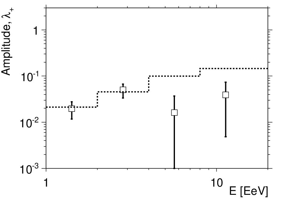
The amplitudes $\overline{r}(E)$, $\overline{\lambda}_{+}(E)$ and $\overline{\beta}(E)$ are shown in Fig. 9 as functions of energy. Dipole amplitudes are compatible with expectations from isotropy. Compared to the results on the dipole obtained in previous section for $\ell_{\mathrm{max}}=1$, the sensitivity is now degraded by a factor larger than 2 as expected from the dependence of the resolution $\sigma_{\ell m}$ on $\ell_{\mathrm{max}}$ (cf Eqn. 17). In the same way as for dipole amplitudes, the 99% $C.L.$ upper bounds on the quadrupole amplitudes that could result from fluctuations of an isotropic distribution are indicated by the dashed lines. They correspond to the amplitudes $\overline{\lambda}_{+,99}(E)$ and $\overline{\beta}_{99}(E)$ such that the probabilities $P_{\Lambda_{+}}(>\overline{\lambda}_{+,99}(E))$ and $P_{B}(>\overline{\beta}_{99}(E))$ arising from statistical fluctuations of isotropy are equal to 0.01. Here, both distributions $P_{\Lambda_{+}}$ and $P_{B}$ are sampled from Monte-Carlo simulations. Throughout the energy scan, there is no evidence for anisotropy. The largest deviation from isotropic expectations occurs between 2 and 4 EeV, where both amplitudes $\overline{\lambda}_{+}$ and $\overline{\beta}$ lie just above $\overline{\lambda}_{+99}$ and $\overline{\beta}_{99}$.

Understanding the influence of the shower size corrections for geomagnetic effects is critical to get unbiased estimates of anisotropy parameters. Without accounting for these effects, an increase of the event rate would be observed close to the equatorial South pole with respect to expectations for isotropy, while a decrease would be observed close to the edge of the directional exposure in the equatorial Northern hemisphere. This would result in the observation of a fake dipole. A convenient way to exhibit this effect is to separate the dipole in two components : the component of the dipole in the equatorial plane $r_{\perp}$, and the component along the Earth rotation axis, $r_{\parallel}$. While $r_{\perp}$ is expected to be affected only by time-dependent effects, $r_{\parallel}$ is on the other hand the relevant quantity sensitive to time-independent effects such as the geomagnetic one.

Estimations of $r_{\perp}$ and $r_{\parallel}$ obtained by accounting or not for geomagnetic effects are given in Table 2, in two different energy ranges. These estimations are obtained from the recovered $\overline{a}_{1m}$ coefficients : $\overline{r}_{\parallel}=\sqrt{3}\overline{a}_{10}/\overline{a}_{00}$, and $\overline{r}_{\perp}=[3(\overline{a}_{11}^{2}+\overline{a}_{1-1}^{2}]^{0.5}/\overline{a}_{00}$. It can be seen that the main effect of the geomagnetic corrections is a shift in $\overline{r}_{\parallel}$ of about 1.2%. In the energy range $1\leq E/[\mathrm{EeV}]\leq 4$, this shift is significant, $\overline{r}_{\parallel}$ changing from -2.2% to -1.0% with an uncertainty amounting to 0.4%. Above 4 EeV, the net correction is of the same order, though the statistical uncertainties are larger. In contrast, $\overline{r}_{\perp}$ remains unchanged in both cases, as expected.

References

- [1] R. U. Abbasi et al. (The IceCube Collaboration), ApJ 718 (2010) 194
- [2] R. U. Abbasi et al. (The HiRes Collaboration), Phys. Rev. Lett. 104 (2010) 161101
- [3] A. A. Abdo et al. (The Milagro Collaboration), ApJ 698 (2009) 2121
- [4] M. Aglietta et al. (The EAS-TOP Collaboration), ApJL 692 (2009) L130-L133
- [5] M. Amenomori et al. (The Tibet AS Collaboration), Science 314 (2006) 439
- [6] R. Beck, Space Sci. Rev. 99 (2001) 243
- [7] V. S. Berezinsky, S. I. Grigorieva, B. I. Hnatyk, Astropart. Phys. 21 (2004) 617625
- [8] V. S. Berezinsky, A. Z. Gazizov, S. I. Grigorieva, Phys. Rev. D 74 (2006) 043005
- [9] P. Billoir, O. Deligny, JCAP 02 (2008) 009
- [10] D. J. Bird et al., (The Fly’s Eye Collaboration), Phys. Rev. Lett. 71 (1993) 3401
- [11] G. R. Blumenthal, Phys. Rev. D1 (1970) 1596
- [12] C. Bonifazi, A. Letessier-Selvon, E.M. Santos, Astropart. Phys. 28 (2008) 523
- [13] C. Bonifazi for the Pierre Auger Collaboration, Nucl. Phys. Proc. Suppl. 190 (2009) 20
- [14] A. Calvez, A. Kusenko, S. Nagataki, Phys. Rev. Lett. 105 (2010) 091101
- [15] J. Candia, S. Mollerach, E. Roulet, JCAP 0305 (2003) 003
- [16] A. H. Compton, I. A. Getting, Phys. Rev. 47 (1935) 817
- [17] D. Cutler, D. Groom, Nature 322 (1986) 434
- [18] D. Eichler, M. Pohl, ApJ 742 (2011) 114
- [19] R. Engel for the Pierre Auger Collaboration, Proceedings of the 30th ICRC, Mérida, 2007
- [20] G. Farrar, R. Jansson, ApJ 757 (2012) 14
- [21] G. Giacinti et al., JCAP 07 (2012) 031
- [22] D. Harari, S. Mollerach, E. Roulet, JCAP 11 (2010) 033
- [23] J. Hersil et al., Phys. Rev. Lett. 6 (1961) 22
- [24] A. M. Hillas, Phys. Lett. 24A (1967) 677
- [25] C. C. H. Jui et al. (The Telescope Array Collaboration), Proceedings of the APS meeting, 2011, arXiv:1110.0133
- [26] M. Kachelriess, P. Serpico, Phys. Lett. B 640 (2006) 225-229
- [27] M. A. Lawrence, R. J. O. Reid, A. A. Watson, J. Phys. G 17 (1991) 733
- [28] T.-P. Li, Y.-Q. Ma, ApJ 272 (1983) 317
- [29] J. Linsley, Proceedings of the 8th ICRC, Jaipur, vol. 4, 1963, p. 77
- [30] J. Linsley, Phys. Rev. Lett. 34 (1975) 221101
- [31] H. J. Mathes for the Pierre Auger Collaboration, Proceedings of the 32nd ICRC, Beijing, 2011
- [32] M. Nagano et al., J. Phys. G 18 (1992) 423
- [33] R. Pesce for the Pierre Auger Collaboration, Proceedings of the 32nd ICRC, Beijing, 2011
- [34] The Pierre Auger Collaboration, Nucl. Instr. and Meth. A 523 (2004) 50
- [35] The Pierre Auger Collaboration, Phys. Rev. Lett. 101 (2008) 061101
- [36] The Pierre Auger Collaboration, Astropart. Phys. 32 (2009) 89
- [37] The Pierre Auger Collaboration, Phys. Lett. B 685 (2010a) 239
- [38] The Pierre Auger Collaboration, Nucl. Instr. and Meth. A 613 (2010b) 29
- [39] The Pierre Auger Collaboration, Phys. Rev. Lett. 104 (2010c) 091101
- [40] The Pierre Auger Collaboration, Astropart. Phys. 34 (2011a) 627-639
- [41] The Pierre Auger Collaboration, JCAP 11 (2011b) 022
- [42] The Pierre Auger Collaboration, in preparation (2012a)
- [43] The Pierre Auger Collaboration, submitted to ApJ (2012b)
- [44] M. S. Pshirkov et al., ApJ 738 (2011) 192
- [45] V. Ptuskin et al., Astron. Astrophys. 268 (1993) 726
- [46] F. Sanchez for the Pierre Auger Collaboration, Proceedings of the 32nd ICRC, Beijing, 2011
- [47] P. Sommers, Astropart. Phys. 14 (2001) 71
- [48] K. O. Thielheim, W. Langhoff, J. Phys. A (1968) 694
- [49] V. N. Zirakashvili et al., AstL. 24 (1998) 139