On the Markov Chain Tree Theorem in the Max Algebra
Abstract
The Markov Chain Tree Theorem is extended to the max algebra and possible applications to ranking problems are discussed.
Keywords: Markov chains, Stochastic matrices, directed spanning trees, max algebra, Kleene star, ranking.
AMS classification 60J10, 68R10, 15B51, 05C05, 15A80, 91B06, 91B12.
1 Introduction
The Matrix Tree Theorem for Markov chains (referred to as the Markov Chain Tree Theorem) is a well-known result that relates the stationary distribution of an irreducible Markov chain with the weights of directed spanning trees of its associated digraph. For a directed graph and , a spanning subgraph of is said to be an -tree if the following conditions are satisfied:
- (i)
for every in , there is exactly one outgoing edge whose beginning node is ;
- (ii)
there is no edge whose beginning node is ;
- (iii)
the subgraph contains no directed cycle.
We now recall the classical Markov Chain Tree Theorem. denotes the weighted directed graph associated with an irreducible matrix ; consists of the nodes with a directed edge from to of weight if and only if . We say the edge is outgoing from and write . Given an -tree in , the weight of is given by the product of the weights of the edges in and is denoted by or just by when is clear from the context.
For , define to be the set of all -trees of . The classical Matrix Tree Theorem for Markov chains, also known as the Freĭdlin-Wentzell formula [1, 2], can be stated as follows.
Theorem 1.1.
Let be an irreducible (row) stochastic matrix. Define by
Then . In particular, is the unique stationary distribution of the Markov chain with transition matrix .
This core result has appeared in a variety of different contexts [1, 3, 4, 5, 6]. It was discovered by Shubert [7] in connection with flow-graph methods, and independently by Kohler-Vollmerhaus [8] motivated by problems in biological modelling. For another reference which discusses its extension to general, not necessarily irreducible Markov chains, see Leighton-Rivest [9].
One of the primary contributions of this paper is to extend the Matrix Tree Theorem for Markov chains to the setting of the max algebra. We show this in two ways; first, we prove a max-algebraic version of the Markov Tree Theorem directly; we then provide an alternative proof using dequantization. We also describe some specific results in connection with the max-algebraic spectral theory. In keeping with Bapat [10], the max algebra consists of the non-negative real numbers equipped with the two operations and . These operations extend to nonnegative matrices and vectors in the standard way [10, 11, 12, 13].
The layout of the paper is as follows. In Section 2, we obtain the Matrix Tree theorem in the max algebra, and we also give an alternative proof using dequantization. In Section 3, we show how to associate our main result with the max-algebraic spectral theory. In particular, we consider the connection with the Kleene star of an irreducible max-stochastic matrix. In Section 4, we discuss the possibility of applying these results to decision making problems. Finally, in Section 5, we present our conclusions and future prospects.
2 Markov Chain Tree Theorem
In this section, we first show that Theorem 1.1 extends to the max algebra. We then provide a second alternative proof of this result using dequantization.
2.1 Markov Chain Tree Theorem in Max Algebra
In the main result below, we present a max-algebraic version of the Matrix Tree Theorem for Markov chains.
Let us first recall standard observations on graphs and spanning trees.
Lemma 2.1.
Let be a digraph and be a node of , to which every other node can be connected by a path. Then contains an -tree.
Corollary 2.1.
If is irreducible then for each node there exists an -tree in with nonzero weight.
Lemma 2.2.
Let be a digraph, be a node of and be an -tree. Then for each node of , there exists a unique directed path from to in .
We now consider an irreducible matrix in which is row stochastic in a max-algebraic sense. Formally, we assume that for , or using max-algebraic notation
In a convenient abuse of notation, we refer to matrices satisfying the above condition as max-stochastic. Our main result shows that Theorem 1.1 extends in a natural way to the max-algebra.
Theorem 2.1.
Let be an irreducible max-stochastic matrix. Define the vector by
| (1) |
Then
Proof.
We first show that . To this end, let an arbitrary be given. Then as , it is immediate that . Now consider such that . Let be a -tree such that , let be the set of edges of and . Consider the set of edges formed by removing from and inserting instead, and denote it by . Consider the subgraph . Note that there is exactly one outgoing edge from every and no outgoing edge from . Further, is acyclic as any cycle in must contain the edge (otherwise it would define a cycle in the original -tree ); however there is no outgoing edge from in . It follows that the graph is an -tree. By construction and since all entries of a max-stochastic matrix are not greater than , we obtain that
and since we were given an arbitrary and took an arbitrary such that , it follows that .
To complete the proof, we show that . Let an arbitrary be given, and let be an -tree such that . As is a max-stochastic matrix by assumption, we know that for some . If then . So let . To show that we will construct a -tree such that . Consider a path connecting to in . By Lemma 2.2 this path is unique. Let be the penultimate node on this path, meaning that . Removing the edge from and inserting the edge we obtain the edge set and the required -tree . Indeed, there is exactly one outgoing edge from each node other than in , and there is no outgoing edge from . Furthermore, if there exists a cycle in , it must contain the edge as otherwise it would define a cycle in . This would then imply that there exists a directed path in from to , all of whose edges are also edges in . This is impossible however, as the only such path in contains the edge which is not an edge in . Therefore is indeed a -tree, which satisfies by construction. Hence and , as was arbitrary. The proof is complete. ∎
2.2 Proof by dequantisation
In this subsection, we present an alternative proof of Theorem 2.1 using a procedure that can be seen as an instance of the Maslov dequantization [14]. Note that the same procedure was used by Olsder and Roos [15] to derive max-algebraic analogues of the Cramer and Cayley-Hamilton formulae.
For , consider the set of nonnegative numbers equipped with the operations and . For , this is a semiring isomorphic to the semiring of nonnegative numbers with the usual arithmetic, via the mapping . We denote by the semiring of nonnegative real numbers equipped with the operations , defined above. We say that is -stochastic if for .
The RST vector of defined as in Theorem 1.1 using the arithmetics of will be denoted by , and when defined in (i.e., the maximal RST vector), by .
Theorem 2.2.
Let be max-stochastic. There exists an integer and a sequence in , where each is -stochastic, such that and .
Proof.
Let denote the set of matrices such that for all and such that if and only if . We start by constructing a nondecreasing sequence of -stochastic matrices .
As is max-stochastic, for each there are entries , where . We denote the other entries in each row by for each . Choose so that
for all . Then for , define by
where
It is readily verified that -stochastic and that for all .
Denoting we obtain
| (2) |
for all and . As for all , it follows that the right hand side of (2) converges to as tends to infinity. Hence converges to .
Next, note that
| (3) | ||||
Since , we see that
| (4) |
where is the number of -trees in (or ).
It is obvious from the definition of that . Let be an -tree such that . It follows that . Then
| (5) |
Let be the edges in the -tree . Then, it follows from (5) that
| (6) | ||||
where is a fixed constant that depends only on the entries of .
As we showed above that as and as , the claim follows. ∎
As each of the semirings is isomorphic to the nonnegative real numbers with the usual operations, it follows from the classical Markov Chain Tree Theorem 1.1 that for all . Passing to the limit and applying Theorem 2.2 yields another proof of Theorem 2.1.
We next present some numerical examples to illustrate Theorem 2.1.
Example 2.1.
| (7) |
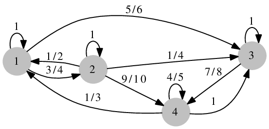
Let be an -tree with the maximum weight for Then,
- •
- •
- •
- •
Hence, and .
3 Maximal RST vector and Kleene star
We have seen that the maximal RST vector associated with the directed graph is always a left max eigenvector of an irreducible max-stochastic matrix . However, in contrast to the conventional algebra, the irreducibility of is not sufficient to guarantee uniqueness (up to scalar multiple) of the max eigenvector. This naturally leads to the question of how to identify the maximal RST vector using the tools of max spectral theory such as the power method or Kleene star. We next consider this question.
First, recall that for with the series converges to a finite matrix called the Kleene star of given by
where [11, 12, 13, 16, 17]. Here, denotes the max-algebraic power of and is the maximum weight of a path from to of any length in (if ). In particular if is irreducible, then is positive [11, 12].
A cycle with the maximum cycle geometric mean is called a critical cycle [10, 11, 12, 13, 16, 17]. The set of nodes that lie on some critical cycle are said to be critical nodes and denoted by . The set of edges belonging to critical cycles are said to be critical edges and denoted by . The critical matrix of [18, 19], , is formed from the submatrix of consisting of the rows and columns corresponding to critical nodes as follows. Set if lies on a critical cycle and otherwise. Moreover, we use the notation for the critical graph of , the digraph which consists of all critical nodes and edges.
The following well-known result shows the connection of with the max eigenvectors of [10, 12, 19]. We adopt the notation for the row, and the notation for the column of the matrix .
Proposition 3.1.
Let be an irreducible matrix with . Assume that has strongly connected components. Then, the following are true.
- (i)
is the only max eigenvalue of ;
- (ii)
is a (right) max eigenvector associated with for ;
- (iii)
For (), and are scalar multiples of each other if they belong the same strongly connected component in .
If one takes columns of from different strongly connected components of , then none of them can be expressed as a max-linear combination of the other columns. Moreover, any such set is strongly linear independent in the sense of [13]. For general (reducible) matrices, is the biggest eigenvalue.
A max-stochastic matrix has max eigenvalue , and for all . This implies that , and that for . Such matrices are called visualized [20]. Note that the max-stochastic matrices have an additional property: each node has an outgoing edge with weight . The spanning subgraph of consisting of the edges of weight defines the saturation digraph, denoted .
Observe that for any matrix with a positive eigenvector , the matrix , where is a diagonal matrix formed from , is max-stochastic. An analogous property holds in nonnegative algebra, where it has many applications, and one can consider a generalization to semifields (i.e., semirings with invertible multiplication). Thus a max-stochastic matrix can be considered to be “eigenvector-visualised”.
The Kleene star of a visualised matrix with (and hence of a max-stochastic one) has a very specific structure, as described, for example, in Proposition 4.1 of [20], which we now recall. Define to be the directed graph formed by adding trivial graphs each consisting of just one non-critical node to (we add one such graph for each non-critical node). We assume that has strongly connected components with node sets .
For , denote by the submatrix of formed from the rows with indices in and from the columns with indices in . Let be the matrix with entries , and let be the matrix with all entries equal to .
Proposition 3.2 ([20], Proposition 4.1).
Let be a visualised matrix, and be the number of strongly connected components of . Then
- 1.
for all and (resp. for ), where );
- 2.
for , the corresponding submatrix of , , where is the -entry of , and is the -submatrix of .
We proceed with the following preliminary result.
Lemma 3.1.
Let be an irreducible max-stochastic matrix. Then, for , .
Proof.
Let be given. It is immediate that
| (8) |
To show the reverse inequality, consider some . We claim that there exists a path from to some of weight 1. As is max-stochastic, there exists at least one outgoing edge from of weight 1, . Moreover, as is not critical, . If is critical, we are done. If not, then there exists with . Continuing in this fashion, we must eventually arrive at some node which was already on the path. Hence this node is on a critical cycle, and is in . By construction, is a path of weight , which we denote by .
Recall that for a max-stochastic matrix , each node has an outgoing edge with weight . The spanning subgraph of , which contains the edge if and only if is known as the saturation subgraph of .
Lemma 3.2.
Let be an irreducible max-stochastic matrix. Assume that is strongly connected. Let be the maximal RST vector of . Then for all , .
Proof.
Evidently for all , since it is obtained by multiplication of the entries of , all not exceeding . To show the lemma we need to construct, for a given critical node , an -tree in . In , each node is connected to a critical node, but if is strongly connected, then any such node is connected to . The proof now follows from an application of Lemma 2.1. ∎
In the next result, we denote by the critical subvector of , i.e., the subvector corresponding to indices in .
Theorem 3.1.
Let be an irreducible max-stochastic matrix and be the maximal RST vector of . Then, the following are true.
- (i)
;
- (ii)
If is strongly connected then ;
- (iii)
If has no more than two components then .
Proof.
(i): Consider a -tree (), with weight . There exists a path in from to for , , with weight . Then,
Thus, , or equivalently (by Lemma 3.1), we have .
(ii): In this case the eigencone is a single ray, consisting of the multiples of a column of Kleene star with index in . Let be equal to any such column. By Proposition 3.2, all the components of equal , and by Lemma 3.2 all the components of equal . Hence .
(iii): Let consist of two components, with sets of nodes and respectively. By Proposition 3.2, there exist and such that , , and . Hence we need to show that when and when . We will give a proof only for , the other case being similar.
As we showed in part (i) that , it suffices to build a spanning tree of weight , directed to . Consider a path of greatest weight connecting a node in to ; by Proposition 3.2 this weight is equal to . Let be the first node on where it leaves and let be the first node on where it enters . By optimality of , only the subpath of connecting to may have weight less than , and this weight is . Using Lemma 2.1 , construct an -tree in the first component of (with node set ), and a -tree in the second component of (with node set ). This makes a spanning tree on the graph consisting of and , directed to . We need to complete this tree to an -tree and having the same weight. We can do this using the edges of , since all remaining nodes of can be connected by a path with edges in either to a node of or to a node of . The resulting tree is directed to and has weight . ∎
It follows immediately that if all nodes in are critical and has two strongly connected components, then the maximal RST vector is given by We now describe some numerical examples to illustrate the above results.
Example 3.1.
Consider the matrix given in (7). There exist three strongly connected components in and such that , and . The Kleene star of is given by
The left max eigenvectors are and .
Then,
However, as there are three strongly connected components in .
4 Application to AHP: discussion
The results of the previous sections relate the eigenvectors of max-stochastic matrices with the maximal weights of spanning trees in the associated directed graph. In this section, we discuss possible applications of these results to questions related to the construction of ranking vectors in decision-making processes. We first note the following simple observation.
Proposition 4.1.
Let , and let the diagonal matrix given by
have all entries nonzero. Further let be the maximal RST vector for . Then
Proof.
Let . Then is irreducible and max-stochastic. For , consider a spanning tree in rooted at . It is clear that the weight of takes the form
where . In fact, it is clear that there is a bijective correspondence between spanning trees in rooted at and spanning trees rooted at in with
It follows that if we write for the maximal RST vector of , then
| (10) |
As is max-stochastic, we know from Theorem 2.1 that . Noting that , we can use (10) to rewrite this as
The result follows immediately. ∎
Now suppose that is a symmetrically reciprocal matrix (SR-matrix), so that for all . Such matrices arise as a result of pairwise comparisons in the Analytic Hierarchy Process (AHP), which is a widely used framework for decision making. The typical interpretation is that indicates the relative strength (or score) of option to option . A central question in the AHP is to determine a weight vector in which represents the weight given to option . Saaty [21] suggested to take to be the Perron vector of . Elsner and van den Driessche [22, 23] suggested selecting from the set of vectors, including the max-algebraic eigenvector, that minimises the functional
| (11) |
Recall that the set of vectors that minimise (11) is the subeigencone of with respect to for an SR-matrix [24].
In this context, a spanning tree in rooted at represents an accumulation of relative scores with respect to all other options in . With this in mind, the vector of maximal RST weights for is a reasonable choice of ranking vector. From Proposition 4.1, we know that must solve the generalised max-eigenvector equation
where is diagonal and satisfies It is worth noting that such a does not minimise the maximal relative error functional in (11) and may give different rankings to the schemes considered there. On the other hand, it has the advantage that the maximal RST vector is unique, while the optimisation problem studied in these earlier papers may give rise to multiple rankings.
Another scenario in which these results could be applied is as follows. Suppose we have a set of “judges” and “competitors”. Each judge is asked to give the competitors a score between 0 and 1 with the highest ranked competitor scoring a and the others scored accordingly. Moreover, each competitor is asked to score the judges in the same way. The judges scores will generate a matrix with a row for each judge, while the competitors’ scores will generate a matrix with a row for each competitor’s scores.
Consider now the matrix . For , consider the entry . Each product can be viewed as an indirect score given by competitor to competitor via judge . Thus the entry is the maximal such score over all judges. It is easy to see that the matrix will be max-stochastic. The maximal RST vector associated with can be used to rank the competitors and Theorem 2.1 shows that is a max eigenvector of . Similar remarks apply to the matrix .
5 Concluding Remarks
We have shown that the Markov Chain Tree Theorem extends to the max algebra. We have also shown that this fact follows from the classical result via dequantisation. We have related the maximal RST vector to the entries of the Kleene star and briefly discussed some possible applications of these results to AHP and ranking.
In an ongoing work, we are going to generalize the Markov Chain Tree Theorem to commutative semirings, and consider the computational complexity of computing the RST vector in this general setting.
References
- [1] M. I. Freĭdlin and A. D. Wentzell. Perturbations of Stochastic Dynamic Systems. Springer-Verlag, New York, 1984. (translation of Russian edition, Nauka, Moscow, 1979.)
- [2] I. Sonin. The state reduction and related algorithms and their applications to the study of Markov chains, graph theory, and the optimal stopping problem. Advances in Mathematics, 145:159–188, 1999.
- [3] V. Anantharam and P. Tsoucas. A proof of the Markov chain tree theorem. Statistics & Probability Letters, 8:189–192, 1989.
- [4] A. Broder. Generating random spanning trees. 30th Annual Symposium on Foundations of Computer Science, 442–447, 1989.
- [5] D. J. Aldous. The random walk construction of uniform spanning trees and uniform labelled trees. SIAM Journal on Discrete Mathematics, 3:450–465, 1990.
- [6] J. R. Wicks. An algorithm to compute the stochastically stable distribution of a perturbed markov matrix. Ph.D. Thesis, Brown University, Providence, RI, USA, 2009.
- [7] B. O. Shubert. A flow-graph formula for the stationary distribution of a Markov chain. IEEE Transactions on Systems, Man, and Cybernetics, 5:565–566, 1975.
- [8] H. -H. Kohler and E. Vollmerhaus. The frequency of cyclic processes in biological multistate systems. Journal of Mathematical Biology, 9:275–290, 1980.
- [9] F. T. Leighton and R. L. Rivest. The Markov chain tree theorem. Massachusetts Institute of Technology, Laboratory for Computer Science Technical Report, MIT/LCS/TM-249, 1983.
- [10] R. B. Bapat. A max version of the Perron-Frobenius theorem. Linear Algebra and its Applications, 275/276:3–18, 1998.
- [11] R. A. Cuninghame-Green. Minimax Algebra. Lecture Notes in Economics and Mathematical Systems, 166, Springer-Verlag, Berlin-New York, 1979.
- [12] F. Baccelli, G. Cohen, G. J. Olsder and J. -P. Quadrat. Synchronization and Linearity. An Algebra for Discrete Event Systems. Free Web Edition: http://www-roc.inria.fr/metalau/cohen/documents/BCOQ-book.pdf, 2001.
- [13] P. Butkovič. Max-linear systems: Theory and Algorithms. Springer-Verlag London Ltd., London, 2010.
- [14] G. L. Litvinov and V. P. Maslov. The correspondence principle for idempotent calculus and some computer applications. Idempotency, 11:420–443, Cambridge University Press, Cambridge, 1998.
- [15] G. -J. Olsder and C. Roos. Cramer and Cayley-Hamilton in the Max Algebra. Linear Algebra and its Applications, 101:87–108, 1988.
- [16] B. A. Carré. An algebra for network routing problems. Journal of the Institute of Mathematics and its Applications, 7:273–294, 1971.
- [17] G. J. Olsder and J. van der Wounde. Max Plus at Work. Modeling and Analysis of Synchronized Systems: A Course on Max-Plus Algebra and Its Applications. Princeton University Press, Princeton, NJ, 2006.
- [18] L. Elsner and P. van den Driessche. On the power method in max algebra. Linear Algebra and its Applications, 302/303:17–32, 1999.
- [19] L. Elsner and P. van den Driessche. Modifying the power method in max algebra. Linear Algebra and its Applications, 332/334:3–13, 2001.
- [20] S. Sergeev, H. Schneider and P. Butkovič. On visualization scaling, subeigenvectors and Kleene stars in max algebra. Linear Algebra and its Applications, 431:2395–2406, 2009.
- [21] T. L. Saaty. A scaling method for priorities in hierarchical structures. Journal of Mathematical Psychology, 15:234–281, 1977.
- [22] L. Elsner and P. van den Driessche. Max-algebra and pairwise comparison matrices. Linear Algebra and its Applications, 385:47–62, 2004.
- [23] L. Elsner and P. van den Driessche. Max-algebra and pairwise comparison matrices II. Linear Algebra and its Applications, 432:927–935, 2010.
- [24] B. Benek Gursoy and O. Mason and S. Sergeev. The Analytic Hierarchy Process, Max Algebra and Multi-objective Optimisation. arXiv:1207.6572v1, 2012.