BPS Degeneracies and Superconformal Index in Diverse Dimensions
Abstract
We present a unifying theme relating BPS partition functions and superconformal indices. In the case with complex SUSY central charges (as in in and in ) the known results can be reinterpreted as the statement that the BPS partition functions can be used to compute a specialization of the superconformal indices. We argue that in the case with real central charge in the supersymmetry algebra, as in in (or the in ) the BPS degeneracy captures the full superconformal index. Furthermore, we argue that refined topological strings, which captures 5d BPS degeneracies of M-theory on CY 3-folds, can be used to compute 5d supersymmetric index including in the sectors with 3d defects for a large class of 5d superconformal theories. Moreover, we provide evidence that distinct Calabi-Yau singularities which are expected to lead to the same SCFT yield the same index.
1 Introduction
Supersymmetric BPS states have played an important role in many aspects of string theory. Their mass is typically protected by SUSY and provides a tool to analyze various limits of string theory. On the other hand superconformal theories have also figured prominently in many developments of string theory. As we deform conformal theory away from the conformal point, BPS states arise in the resulting theory. It is natural to ask what is the relation between BPS states that appear and the properties of the superconformal theory they come from. In fact there is evidence that the BPS spectrum away from the conformal point is faithful, and the superconformal theories are entirely captured by the BPS spectrum. In particular, we do not have a single example of two distinct superconformal theories which give the same BPS spectrum upon deformation. Of course, not arbitrary BPS spectrum gives rise to a consistent theory, and consistency conditions on what the allowed BPS states can be, has been proposed as a way to classify conformal theories for in [1] and in [2, 3] . If this is the case, it should be possible to recover all the data at the conformal fixed point solely from the BPS data. In particular it is natural to ask if the superconformal partition functions such as supersymmetric indices [4, 6, 5] are reproducible from the BPS spectrum.
The most natural idea would be to treat BPS states as if they are the elementary building blocks of the theory and use them to compute the superconformal partition functions. However the story is not always so simple. For example for theories with complex central charge, the BPS spectrum has different chambers separated by walls. Nevertheless, as we will review (and partially reinterpret), it is known that at least in the cases of with [2] and with [7] a specialization of the superconformal index can be recovered from BPS spectrum in any chamber.
We will provide evidence that the situation is similar but more powerful in the case of theories in dimensions with Coulomb branch, with supersymmetries respectively. Both of these cases involve a real central charge. In these cases we propose that one can recover the full superconformal index solely from the BPS data in a Coulomb branch of the theory. In the case of we reinterpret the computations already done as computing contributions from BPS states. The main new case involves the superconformal index in .
The basic class of examples we consider is obtained from M-theory on Calabi-Yau threefolds leading to theories in dimensions. It is known that for these cases the topological string captures the BPS degeneracies (corresponding to M2 branes wrapping 2-cycles) [8, 9]. In addition one can introduce M5 branes wrapping Lagrangian submanifolds of Calabi-Yau. These lead to 3 dimensional defects in the 5d theory. Furthermore it is known that open topological strings captures the open BPS state degeneracy for these sectors corresponding to M2 branes ending on M5 branes [10, 11]. We will argue that superconformal index, i.e. the partition function on where the 3d defects wrap where , can be computed simply by considering
where is the refined open and closed topological string amplitudes, correspond to the Wilson line associated with nomalizable Kähler moduli of Calabi-Yau, is the non-normalizable Kähler moduli, which correspond to mass parameters, correspond to the Wilson lines for the Lagrangian branes and are the two coupling constants of the refined topological string. Here complex conjugation sends11 1 As we will discuss later, for the defect sector we can turn on monopole flux which would correspond to allowing to be complex. . Furthermore this computation can be viewed as computing the scattering amplitudes of a string theory in 4 dimensions proposed recently [12].
A unifying theme seems to emerge about the connection of BPS states to the index, which can be summarized roughly as follows: We order the BPS states according to the phase of their BPS central charge. In the case of real central charge this simply means dividing the BPS states to CTP conjugate pairs where one half of the states are on right and the other on the left of the real line. In the case of complex central charge this means organizing the states on a circle according to the phase of the central charge where CTP conjugate pairs are diametrically opposite. Whether it is real or complex central charge we can consider a ‘partition function’ of the BPS states where each BPS state is represented by an operator and we take the product over all the BPS states. The operator acts on a different Hilbert space depending on the dimension and the theory in question: In the 2d case it involves the space of massive vacua, in the 3d and 5d cases it is the space of flat connections on for the corresponding abelian gauge groups, and in the 4d case it is the Hilbert space of a Chern-Simons theory on the Seiberg-Witten curve.
In the complex central charge case do not commute and we have to order them according to the phase of the central charge in the SUSY algebra. In the real central charge case they commute. Moreover knowing the contribution for half the states is sufficient, because the CTP conjugate case can be obtained from them. Let
denote the (ordered) product over the BPS states whose phase is on one side. The full partition over BPS states will take the form
| (1) |
Then the statement is that
| (2) |
for suitably defined partition function of the theory on . For this gives the full index and for this gives a specialization of the index.
The intuitive idea for why such a picture holds may be that we can view operators at the conformal fixed point as being made of the composite of operators which create BPS states. In some cases where there is a weak coupling description of the theory, as in gauge theories, this picture can be fully justified.
The fact that we propose that the superconformal index in 5 dimensions can be computed only from the knowledge of BPS particles is surprising in the following sense: These theories also have BPS strings. If we go to the conformal point, we will have a system of interacting massless particles and tensionless strings. Upon going to the Coulomb branch the particles pick up mass and tensionless strings pick up tension. Moreover the mass scale for both the interacting strings and the particles are the same [13]. What is surprising is that nevertheless the knowledge of only BPS particles is enough to recapture the full superconformal index in 5 dimensions. Perhaps this can be explained by the fact that has no 2-cycles for the worldsheet of BPS strings to wrap around and the properties of the BPS strings are secretly encoded by the particle states, as far as the index is concerned.
The organization of this paper is as follows. In section 2 we discuss the relation between superconformal indices and BPS states in two and the four dimensional theories with complex central charges. In section 3 we discuss the three and five dimensional gauge theories with real cental charges, superconformal indices and their relation with BPS states including coupling to the 3d defects. In section 4 we review the refinement of topological strings and how the refined amplitudes can be calculated. In section 6 we give some examples of index computations for certain 5D theories coming from local CY threefolds including in the presence of 3d defects. In section 7 we present our conclusions.
2 BPS states and theories with complex central charge in
In this section we review (and partially reinterpret) what is known for the relation between BPS states and superconformal partition functions in the case of theories in and theories in .
2.1 theories in
Consider an conformal theory in . In this context we can define a superconformal index (which is an elliptic genus) [14] given by the following trace in the Ramond sector:
where is the left-moving charge and , being the fermion numbers of the left and the right movers. Since the Ramond sector is supersymmetric, by SUSY argument as in the Witten index, the above index only depends on and is independent of moduli of conformal theory. It receives contributions from all the states which are ground states of the and it is an arbitrary eigenstate of . Note that in the limit this receives contribution only from the ground state . In this case simply computes the partition function of the ground states in the Ramond sector weighted by their R-charge .
We will consider a subset of theories which admit deformations which flow in the IR to a trivial theory. For this to be possible in particular and the ground states have equal charges. The index of such theories, which is also equal to the number of distinct vacua upon mass deformations is .
For special values of , the index simplifies and becomes -independent: Let
note that since is not necessarily an integer, putting is not the same as . Moreover in this limit the left-moving supercharges also commute with the elements in the trace and the partition function is independent, and in particular can be evaluated by taking the limit:
In particular as shown in [15] using spectral flow, counts the index of the theory relative to , where refer to (left,right)-moving supercharges in the Ramond sector.
This theory will have BPS kinks connecting the various vacua. The number of kinks depends on how we deform the superconformal theory to the massive ones, and there are domain walls in parameter space where the BPS degeneracies change [16]. Let be the number of kinks connecting the -th vacuum to the -th one, taking into account the acting on the lowest state of the multiplet. BPS kinks come with complex central charges. Order the vacua such that the phase of the corresponding central charges goes counter-clockwise as we increase . In this basis let be the upper triangular matrix given by for each . Consider the matrix
and furthermore construct the matrix
| (3) |
where is the inverse transpose of . Since is upper triangular we have
Wall crossing formula for the BPS states [16] imply that the eigenvalues of do not depend on which chamber we compute it in (even though does change). So it is purely a property of the conformal fixed point. Moreover, using equations [17] it was shown in [1] that22 2 Furthermore it was shown how this can be refined to compute the for arbitrary .
| (4) | |||||
Moreover this was used as a starting point of a program to classify theories in . For a recent discussion of the meaning of this relation see [18].
An Example: As an example consider the case of LG theory with superpotential for which a conformal fixed point is expected [19, 20]. The spectrum of the R-charges at the conformal point is . The chiral ring consists of and when the theory is deformed so that the superpotential becomes we get two vacua for . There is a single BPS kink connecting them therefore
![[Uncaptioned image]](1210.3605v3/kinks.png)
has two eigenvalues which agrees with the spectrum of the R-charges of the theory at the conformal point.
It is interesting to note that Eq.(3) has the structure of the partition function of fermions and bosons. It is as if we are constructing composite operators from the fields creating the kinks. Moreover consider the kink operators placed on a circle ordered by the phase of their central charge and the ones on the left semi-circle are fermionic and the ones on the right-half are bosonic. Then the can be viewed as the totality of operators we can make out of them which can be placed on a circle (i.e. start from one vacuum and end on the same vacuum). This structure will repeat, as we shall see in all the other dimensions where we connect BPS degeneracies with partition functions at superconformal points.
2.2 BPS states and , in dimensions
The connection between degeneracies of BPS states for theories in and certain partition functions at the superconformal point was found in [7]. We consider the theory in the background involving where is the Melvin cigar: is given by where we rotate by as we go around . Moreover as we go around the other we twist by where is the extra r-charge which is a symmetry at the conformal point and is a Cartan in the . The can be viewed topologically as with squashing parameter . We will denote this by
One considers the partition function on which can be represented in the operator formulation as (suppressing the irrelevant )
| (8) |
We now explain the relation of this partition function with the deformed theory. Each BPS state is characterized by a charge which belongs to the lattice of electric and magnetic charges. Note that this lattice has a canonical skew-symmetric product pairing the electric with the corresponding magnetic charges. Consider the quantum torus algebra given by introducing for each element of the lattice an operator satisfying33 3 When the , theory is realized in terms of an M5-brane wrapping inside a CY3fold, being the time direction, then BPS states are given by M2-branes bounding and is the holonomy of the gauge field coming from the B-field on the M5-brane reduced along the cycles of [7].
For each BPS state of charge and spin introduce the operator
| (9) |
Consider BPS states whose central charges lie on the upper half-plane.
| (10) |
where denote ordering the product in the order of the phases of the central charges as it goes in a counter-clockwise direction. Furthermore consider the matrix
as in the 2d case, where the inverting of means replacing and , and taking the inverse of the products. Furthermore transposition means the order in the product continues in the order of increasing phase of central charge. It was found in [7] that
| (11) |
The fact that this gives the same result in all chambers follows from the work of Kontsevich-Soibelman [21] and its refinement [22]. The similarity of the setup to the 2d case is striking and was explained in [7]. For alternative derivation see [23].
It is tempting to connect this to more standard superconformal index. In fact as noted in [7, 25, 24, 26] if we consider the double space , the partition function on this space gets related to a doubled version of BPS contributions given by
where with the parameterizations , and . It can be checked that satisfy
Moreover and commute. Then, it was proposed in [7] that if we consider
where is constructed out of , then
It is natural to compare this with the usual superconformal index. Given the relation between superconformal index in 4d and the partition function on squashed [27, 28, 29], it is natural to propose44 4 The combination was suggested by the relation with topological strings. However, the correct relation was recently found in [30] and is given by , which is and limit of the superconformal index.
which can be viewed as a special limit of the superconformal index:
with the specialization .
3 BPS states and gauge theories with real central charges in
In this section we review the computations done for the superconformal index for gauge theories with in and in . In both cases we argue that they can be written entirely in terms of BPS states of the corresponding theories in the Coulomb branches. This reinterpretation leads to our general proposal for relation between BPS states and the index for all superconformal theories in .
3.1 Superconformal index in , N=2
Here we review the basic statement for computation of superconformal index for gauge theories on [31, 32, 33, 26].
Consider a 3d theory with gauge group , and some matter representations . Moreover, depending on what interactions are turned on, certain flavor symmetries can be introduced. The superconformal index can be viewed as computation of
where is the rotation generator on , denotes the R-charge and are some flavor charges. The basic statement is that we can compute simply by taking the contribution of all the fields in the UV to the index, where it can be taken to be a weakly coupled theory. Since the index does not change upon flow, this would give the superconformal index at the conformal point as well. If we have gauge group factors we can turn on flat connections on , which we denote by , which need to be integrated over. This is equivalent to projecting to gauge invariant fields. Moreover, for each flavor charge we introduce a fugacity around the circle.
The contribution for each particle splits up formally to a square due to CTP structure of each multiplet. Let be the contribution of one of the particles. Let the spin of the particle be , and charges under the flavor symmetries, and charge under the gauge symmetries. Then55 5 Here we are turning off the fugacity associated with monopole number which can be viewed as complexification of [26].
where is the -charge of the field (and for free theory gets identified with ). Including the CTP conjugate is the same as introducing . Let
Then the index can be written as66 6 The integration is over the Cartan of . This is also true in the non-abelian case where the extra measure factors can be viewed as arising from the contributions of the massive gauge particles of the non-abelian group in the Coulomb branch.
which has the same structure as what we had seen in . Indeed if we go to the Coulomb branch the basic field become BPS states and so this can also be viewed as computation using the BPS states77 7 More precisely what we mean by this is that if we ungauge the ’s, the BPS partition function of the global symmetries determine what are the BPS states. The index for the ’s which we gauge is determined entirely in terms of them., in the same sense as we had seen in . Note that at least formally this can be written in the form
using the fact that (not worrying about regions of convergence of )
This computes the index at zero monopole number. One can also include the effect of the global symmetries associated with shifting the dual photon. This can be done most naturally by considering a generalized index [33] with fixed monopole numbers . This can be shown to be equivalent [26] to viewing holonomies as complex, shifting where is viewed as real and at the end, after taking substituted by .
3.2 , and BPS states
The superconformal index in is defined [5] by the twisted partition function on :
where and are the rotations of two planes in and denotes the Cartan of the R-symmetry, and denote flavor symmetries. The fact that there are non-trivial superconformal theories has been argued from many different viewpoints [34, 35, 36, 13, 37]. There are non-trivial superconformal field theories whose existence is signaled by the existence of massless particles and tensionless strings. Moreover, as argued in [34] many superconformal theories deform upon mass deformations to gauge theories. In turn, in the IR limit the gauge theories become weakly coupled, and one can use this weakly coupled IR theory to compute the index. Since the index is independent of deformations this can be used to recover the index at the conformal point. This idea has been considered in [38] where the superconformal index for some theories were computed using localization techniques. This includes that of with up to fundamental matter. Moreover the expected symmetry of these theories was successfully tested. The basic structure of the answer can be recast, which we discuss in more detail in section 6, as
where denotes the Nekrasov partition function for the 4d theories coming from compactification of the theory on , and denote the holonomy of the gauge group along , and are exponential of mass parameters and the instanton number (which is one of the flavor symmetries). Moreover in the above formula the involves complex conjugating the but keeping unchanged. Of course this result was already anticipated by the computation of Pestun [39] relating 4d Nekrasov partition function with gauge theory partition function on . This can be viewed as a special instance of that general argument where the argument is applied to the 4d theory obtained by compactification from 5d.
The question is what is the relation of this index with BPS states? Unlike the 3d case, where the basic fields can be viewed as BPS states in the Coulomb branch, in the 5d case the gauge fields and matter fields are not the only BPS states. Indeed this is consistent with the fact that is considerably more complicated than the case where the index is given by treating the basic fields as the only relevant ingredients for the computations. Indeed there are infinitely many BPS states in this case. The question is whether can be reinterpreted just in terms of BPS states, as was the case in ?
As is well known the partition function of refined topological strings on a CY which engineers the corresponding gauge theory [40] is identical with Nekrasov’s partition function. Therefore we can interpret the above statement as
On the other hand, it is known that topological strings captures BPS degeneracies [8] (see [9] for the refined version):
where is the BPS degeneracy with spins written in an orthogonal basis of Cartan, gauge charges and flavor charge (where in topological string translate to an element of of CY where the M2 brane wraps to give rise to BPS state). Thus we can view this as a partition function of BPS particles:
with identified as the above, counting the BPS states as if they are the elementary building blocks of the theory, even though there is no weak coupling Lagrangian which describes them as fundamental fields. Nevertheless they seem to behave as such. Moreover is given by
The proof of this is given in section 4 above Eq.(26) when we discuss the properties of the refined partition function.
Therefore we can again write the index as
Thus we have a unified picture in on the relation between BPS states and supersymmetric partition functions.
3.3 Inclusion of codimension 2 defects
In the context of topological strings we can also consider M5 branes wrapping special Lagrangian submanifolds. These correspond to 3d defects in gauge theory, giving the analog of surface operators in the context of 4d gauge theory [41, 42]. We will describe the detailed definition of them shortly. We can then ask how one may compute the index of the 5d theory in the presence of 3d defects. This fits nicely with the above formalism by simply combining the degrees of freedom of the BPS states involving M2 branes ending on M5 branes, which open topological string counts [10, 11]:
where are the bulk and defect holonomies around respectively and are the flavor symmetries. correspond to Kähler classes in the Calabi-Yau. This computes the index in the zero monopole number sector. To obtain the generalized index of [33, 26] with fixed monopole numbers , it suffices to take to have a real piece and substituting, after taking the , , where we have taken the M5-brane to be in the 12-plane.
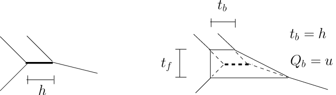
Next we discuss in more detail the connection between M5 branes wrapping Lagrangian submanifolds and gauge theoretic defects (see also [43]). M5 branes wrapped on special Lagrangian submanifolds and filling an in space-time correspond to supersymmetric defects preserving half of the supersymmetries (i.e. leading to supersymmetry in ). We will be mainly considering non-compact Calabi-Yau threefolds which are toric. A distinguished class of special Lagrangian cycles in these cases [44, 45] have the topology of for which a cycle of shrinks at each end. In the compact region of the toric 3-fold, where one cycle of shrinks it ends on the web of the toric diagram. With no loss of generality let us call this the cycle of . At infinity a cycle of the shrinks ending on the ‘spectators brane’. Let us call this direction the . The topology of this Lagrangian submanifold is the lens space which has fundamental group . As discussed in [25] there is an supersymmetric Chern-Simons gauge theory living on the non-compact 3 dimensions of the wrapped M5 brane, with level . Furthermore this theory has a flavor symmetry associated with the monopole number (corresponding to shifting the angular scalar dual to the photon). The corresponds to the Chern-Simons level for this flavor symmetry. Furthermore the position of the brane on the web is determined by the FI-term for the gauge symmetry. Such a defect can be defined for any 5d conformal theory arising from toric CY, where the lines of the web pass through the same point. As the web is resolved through breathing modes of the web, one per cycle, the spectator line where the brane is suspended can intersect a number of edges in the diagram and the brane can end on any of the lines (see Fig 1). In order to make sure the amplitudes is invariant under resolutions, and it is a defect associated to a superconformal theory, we need to sum over all such possible endings.

In case the toric geometry engineers an gauge theory (corresponding to parallel lines, the spectator line will intersect the ladder of parallel lines at any of points, and we will need to sum over all of them. This would correspond to breaking to near the defect position. Moreover as discussed in [42] in the analogous situation of surface defects in 4 dimensions, the surface defect generates a deficit angle in the , proportional to FI-term . We have
corresponding to moving the end brane along the line whose length is , as the brane traverses the line the deficit angle varies from to . As we change the Coulomb branch parameters the effective depends not only on the Coulomb parameter but also on the slope (see Fig 1).
In computing the index in the presence of defect we choose a number of defect spectators with various slopes and some fixed positions (corresponding to their FI-terms ). We can also have more than one brane suspended from each. In the gauge theory setup this will translate to more general patterns of breaking the gauge symmetry near the defect. We then integrate over the breathing modes of the loops (i.e. Wilson lines of the 5d gauge theory), and the Wilson lines associated to the gauge field on the brane, fixing the position of the suspended lines at infinity and the external lines of the web, which collectively play the role of mass parameters.
4 Topological Strings and BPS states
The topological strings propagating on a CY threefold have been intensely studied in recent years from both mathematical and physical viewpoints. They not only provide an exactly solvable sector of the full string theory but also provide very useful insight into the spacetime physics. In this section we will summarize the relation between topological strings on and BPS states which arise in the M-theory compactification on .
Consider a Calabi-Yau threefold and let be the Kähler class. The classes span and we denote with the 4-cycle dual to . The genus A-model topological string amplitude on the Calabi-Yau threefold are then given by [46]
| (12) | |||||
where are the triple intersection number of the divisors dual to , are the genus Gromov-Witten invariants and the is the Chern class of the Hodge bundle over the moduli space of genus curves, , and
| (13) |
In the above equation are the Bernoulli numbers, .
The topological string partition function is given by
| (14) |
where is the topological string coupling constant. In [8] topological strings on a CY threefold were studied from a spacetime point of view and it was shown that the topological string partition function captures the degeneracy of BPS particles in the 5D theory coming from M-theory on . We present a short summary of their argument linking the BPS states in 5D with topological strings. Consider M-theory compactification on CY threefold which gives a 5D theory. The massive BPS particles will form representation of the little group in 5D . These BPS particles in 5D arise from M2-branes wrapping a holomorphic curve in and have mass equal to the area of the curve. These BPS particles are electrically charged under the abelian gauge fields coming from the 3-form ,
| (15) |
As has been mentioned before the 5D theory also has states which are magnetically charged under . These magnetically charged states are not point particles but are strings coming from M5-branes wrapping the 4-cycles in . The M2-brane wrapping a holomorphic curve in the class gives rise to a set of BPS particles in 5D with mass equal to and certain spin content. Let use denote by the number of particles with spin and charge (which determines the mass) and let
| (16) |
The integers are invariant under complex structure deformations of and are the BPS degeneracies captured by the topological strings. In terms of the topological string partition function can be written as
In above the numerator is the classical contribution coming from worldsheet with genus zero and three punctures (the cubic term) the worldsheet with genus one and one puncture. The denominator is the contribution coming from constant maps and can also be written as
| (17) |
where is the generating function of the number of plane partitions known as MacMahon function. Thus the full topological string partition function is given by
There also exist a refinement of the above topological string partition function. Notice that the GV invariants is an index over the Hilbert space of states coming from and the index structure is needed since complex structure deformations can change but do not change . This is the story for generic CY threefold. For local CY threefold (noncompact toric CY threefolds) the story is much more interesting. The local CY threefolds enjoy extra R symmetry and, therefore, are also invariants. The refinement of topological string partition function captures these full BPS degeneracies 88 8 In the previous sections the coupling constants of the refined topological strings were denoted by and . From now on we will denote them by and which are more familiar in the context of calculations involving the refined topological vertex.:
| (18) | |||
where is the refined MacMahon function,
| (19) |
and . The usual topological string partition function is recovered in the limit . Notice that we have kept the classical contribution and the constant map contribution. Eq.(18) can also be written as
| (20) |
where is the Plethystic exponential of defined as
| (21) |
In general for local CY threefold is not well defined, however, if we only consider compact homologies in its definition we get it equal to twice the number of 4-cycles. This is the value we will use in writing the factors of MacMahon function in the refined partition functions.
Before we discuss how the refined topological string partition function can be calculated for local CY threefolds let us discuss an important property of the partition function which has been mentioned before and which will be of importance later. We would like to see how the refined partition function transforms under complex conjugation. In the later calculations of the index, as have been discussed earlier, the Kähler parameters will be taken to be pure imaginary and some of them will be integrated over. Keeping this in mind the complex conjugation acts as follows on the variables ,
| (22) |
Now it is easy to see from Eq.(20) that 99 9 As long as for each we have the full spin content corresponding to . This is indeed the case for the class if the corresponding moduli space of D-brane is compact. A counter example to this is the case of . In this case the moduli space of the is and the corresponding .
| (23) |
The MacMahon function, which is part of the closed topological string partition function, behaves in a non-trivial way under the complex conjugation,
| (24) | |||||
| (25) |
Thus from Eq.(23) and Eq.(25) it follows that
| (26) |
and therefore
| (27) |
where the classical piece cancelled because it was odd in .
Now we will briefly discuss the open string case which will be of use when we consider the 5D index with a 3D defect. In the A-model topological string one can consider worldsheet with boundaries as long as proper boundary conditions are enforced which preserve the A-model supersymmetry. The boundary conditions in this case require the boundary of the worldsheet to end on a Lagrangian submanifold of the target space. These Lagrangian submanifolds on which the worldsheet can have boundaries are the Lagrangian branes of the theory. For the local CY threefolds we are considering these Lagrangian branes are non-compact and have the topology of . The partition function of the A-model in the presence of branes was studied in [10] from a spacetime viewpoint and it was shown that in this case, just as in the case of closed strings, the partition function captures certain BPS degeneracies. The spacetime picture arises if we consider Type IIA compactification and consider a D4-brane wrapped on the Lagrangian cycle. In this D2-branes can wrap holomorphic curves in and end on the D4-brane. The open topological string partition function captures the degeneracies of BPS states arising from D2-branes ending on the D4-brane. If we denote the Lagrangian brane by then the D4-brane wraps where is part of the spacetime . The theory on the has a rotation and a R-symmetry. We combine these two ’s and define and . In addition to these quantum numbers the D2-brane couples to the gauge field on the D4-brane and we can introduce a holonomy factor where is the holonomy of the gauge field on the D4-brane around the nontrivial of . If we denote by the number of particles with charge and quantum numbers in the representation , then the open topological string partition function is given by,
| (28) | |||||
| (29) |
where
| (30) |
The is the fermion number and above index is invariant under complex structure deformations.
A refinement of the above partition function also exists and is given by [11] (see also [55])
| (31) | |||||
| (32) |
The action of complex conjugation on the open string partition function is different than in the case of the closed string partition function that we discussed above. The action of complex conjugation on the open string variables is given by
| (33) |
With this action the Eq.(32) gives
| (34) | |||
Thus for the open string case
| (35) |
An Example: Consider the case of with a Lagrangian brane on the . In this case the open string partition function is given by
Using
| (36) | |||||
it is easy to see that
5 Five dimensional superconformal theories from toric Calabi-Yau threefolds
In this section we briefly recall the class of 5D superconformal theories for which our methods yield the corresponding index. See [12] and references therein for more detail.
We consider M-theory on toric Calabi-Yau threefolds, or equivalently type IIB string theory with a web of 5-branes. Let be the coordinates of the ten dimensional spacetime. The 5-branes fill the part of the spacetime given by and extend as a web of piecewise straight lines in the plane given by and . The generic 5-brane web can be viewed as a trivalent graph in depicting each 5-branes as a line segment in (filling the space-time) where the slope of each line is given by the . The generic graph is trivalent with on each vertex. An example of such a web is shown in Fig. 2.

In the limit where the web becomes singular, consisting of lines all passing through the same point, we get a superconformal theory in 5D. An example is shown in Fig. 3 where the singular web gives a superconformal theory with global symmetry.

The resolutions of the web, fixing the external line, correspond to going to the Coulomb branch of the 5D gauge theory. Some of these theories correspond to gauge theories upon resolutions [47]. However most of them do not have a direct gauge theory interpretation. Our method for computing the index applies equally well to all of them.
Moving the external lines, correspond to changing the mass parameters of the theory. The data of the conformal theory is thus captured by a collection of external lines characterized by 5-branes, with the condition that
Moreover, for each one can introduce a mass parameter corresponding to moving the external lines parallel to itself. They add up to zero and there is in addition a two parameter redundancy due to shifting the origin of the , so the number of mass parameters is 3 less than the number of external lines. It was proposed in [12] that this data can be identified with the states of a 4D string on . Moreover, the scattering amplitudes of the resulting string states are identified with the superconformal index of the resulting theory in 5D:
In addition we can select a number of spectator branes from which the Lagrangian branes can be suspended, giving rise to defects of the 5d theory. The slope of the spectator branes determine the type of defect we introduce. Its position is a mass parameter associated to the FI-term on the defect. These correspond to degrees of freedom of the unwound string in the proposal of [12].
5.1 Loop variables and Kähler parameters
In calculating the index we need to integrate over the loop variables associated with the 4-cycles in the geometry. Each loop variable correspond to a coming from the 4-cycle as discussed in section 4. Since the partition function depends on the Kähler parameters we need to determine how the Kähler parameters depend on the loop variables. This relation can be easily determined either from the web diagram or from the geometry.
Let us first show how we can determine the dependence of the Kähler parameters on the loop variables using the web diagram. Consider an edge which is one of the edges forming the loop (4-cycle) in the web diagram. Let and be the two edges connected with but not part of the loop as shown in Fig. 4 where we have used transformation to convert the edge to a horizontal line.

From Fig. 4 it is clear that as the 4-cycle size changes the size of the edge also changes with it. The relation between the deformation of the 4-cycle given by the change in the loop variable and the change in the size of the edge depends on the slope of the connected edges and and is given by
| (37) |
If we define , the loop variable and let and be the winding vectors associated with and then the invariant version of the relation between the edge variable and the loop variable is given by
| (38) |
where is the value of for and is determined by the position of the external legs.
If the geometry has many 4-cycles then it may becomes difficult to determine the dependence of the Kähler parameters on the loop variables using the web diagram although the basic idea still is same. A more geometric way of obtaining the relation follows from the fact that holomorphic curves in the geometry give rise to BPS particles in the 5D theory which are electrically charged under the gauge group (assuming there are 4-cycles in the geometry). The scaling relation between the Kähler parameter of a curve and the loop variables is just given by the electric charge of the corresponding state:
| (39) |
where are the loop variables corresponding to the 4-cycles and is electric charge of the state coming from under the (the coming from the i-th 4-cycle). The electric charge of the curve is a purely geometric quantity given by the intersection of the curve with the 4-cycle. If we denote the 4-cycles in the geometry by then
| (40) | |||||
| (41) |
where is the anticanonical class of the divisor . We will use Eq.(39) and Eq.(40) to determine the relation between the Kähler parameters and the loop variables when calculating the index in section 6.
6 Computation of the 5d index through topological string
In this section we will calculate the index for certain 5D theories using the refined topological string partition function. The refined partition function will be calculated using the refined topological vertex. We will give a short introduction to the refined vertex formalism
6.1 Refined vertex formalism
The topological vertex, which was derived using large N transition from Chern-Simons theory, can be used to calculate the topological string partition function for a toric CY threefold [48]. A refinement of the topological vertex was found in [49] and allows the calculation of refined topological string partition function for a large class of toric CY threefolds 1010 10 See [50] for an earlier attempt at refining the topological vertex by replacing Schur polynomials with Macdonald polynomials.. The refined topological vertex is given by
where is the skew-Schur function and the following table summarizes other quantities:
Given any web diagram corresponding to a toric Calabi-Yau threefold we give orientation to edge and associate to each internal edge a partition . To each external edge we associate the trivial partition i.e., the empty set. Since in the web diagram three edges meet at each vertex we have a set of three partitions for each vertex. If an edge is oriented such that it is going out from the vertex the corresponding partition is changed to its transpose. We use these three partitions, say associated to the incoming edges of the vertex, to associate with the vertex the refined topological vertex . The ordering of the three partitions in writing the refined vertex is taken to be anticlockwise as we go around the vertex and this should be the same for all vertices in the web diagram. To each edge of the web diagram we had associated a partition and we now associate a factor of where is the length of this edge and is an integer which is determined by the local geometry of the associated to the edge in the CY threefold. In the neighborhood of a in a CY threefold the geometry looks like with , the integer . Another important constraint that needs to be considered in the case of refined topological vertex, but not for the usual topological vertex, is that at each vertex we need to assign one edge as the preferred edge and all preferred edges in the web diagram should be parallel to each other. This constraint comes from the construction of the refined topological vertex in terms of plane partitions and restricts the class of toric CY threefolds to which refined vertex can be applied to those geometries which are fibrations over a or a chain of ’s. In writing the refined vertex for an vertex, of the web diagram, the partition associated with the preferred edge is always the last partition in the refined vertex and the two refined vertex factors which appear for two vertices connected by a preferred edge should have parameters switched between them. With these constraints in place the refined topological string partition function is given by taking the product over all vertices of the corresponding refined vertex factors and taking a product over all edges of the corresponding edge factors and summing over all partitions:
An Example: Consider local , canonical bundle on Hirzebruch surface . The web diagram of this geometry is shown in figure below. We take the two horizontal lines to be the preferred edges.
![[Uncaptioned image]](1210.3605v3/example.png)
| (43) | |||||
The refined partition function is then given by
| (44) |
After some simplification and using the identity we get
| (45) | |||||
6.2 Example 1: Local
Let us begin with a very interesting example of local . This CY threefold gives rise to gauge theory and we will be able to compare the answer we get from topological strings with the gauge theoretic calculation of [38].
The web diagram corresponding to this CY threefold (which is dual to the Newton polygon encoding the toric data of this CY threefold) is shown below in Fig(5).

In the above figure and are related to the Kähler parameters and corresponding to the base , which we will denote by , and the fiber , which we will denote by , respectively as
The refined partition function of this geometry was calculated above and is given by taking in Eq.(45),
| (46) | |||||
The refined topological vertex calculation gives the last factor in Eq.(46). The first factor involving the refined MacMahon function has been added in accordance with Eq.(18) while taking , as discussed in section 5, since there is only one 4-cycles. We have ignored the classical contribution in writing the refined partition function since it cancels when we take the absolute value square of the refined partition function as discussed in section 5.
The the index for this geometry is given by
where is the loop variable (breathing mode) for the 4-cycle in the geometry. In section 6 we discussed the general relation between the Kähler parameters and the loop variable. In this case we see that the is related to loop variable as
| (47) |
also depends on the loop variable and, therefore, on . This dependence can be easily determined using the web diagram. Consider the web diagram shown in Fig. 5. If the external legs are fixed then the two parameters and are not independent anymore, instead the choice of the external legs determines a parameter such that as shown in the Fig. 6.

Thus the index is given by,
We can now use Eq.(46) to determine the above index to obtain 1111 11 The index can also be written as a infinite product (48) where . It would be interesting to see if have a direct physical meaning.:
| (49) | |||||
where and .
In order to understand the relation between the gauge theoretic calculation [38] and topological string result that we just derived we will look carefully at the various factors which arise in the calculation of the index.
In [38] the index for gauge theory with was calculated using equivariant localization and was given by
| (50) |
where is the parameter on the Coulomb branch, is the instanton counting parameter and and are related to the equivariant parameters and for the action of ,
| (51) | |||
The perturbative contribution after subtracting the Haar measure is given by ,
| (52) |
Now we can identify different pieces of the integrand in Eq.(50) with different contribution to the topological string partition function. The topological string partition function of local can be written as
| (53) | |||||
| (54) | |||||
In Eq.(53) is the contribution to the partition function coming from branes wrapping the fiber curve only and is the contribution to the partition function coming from branes wrapping the base curve at least once and wrapping the fiber curve arbitrary number of times. The contribution is such that
| (55) |
Thus in the limit the only contribution to the partition function comes from branes wrapping the fiber curve and the D0-branes (the constant map contribution). gives the perturbative part of the 4D gauge theory partition function in the limit
| (56) |
The index is expressed in terms of the variables and which couple to the and spins. To see the relation between the integrand of the index and the topological string partition function lets express partition function in terms of the variables and :
| (57) | |||||
| (58) | |||||
Similarly
| (59) | |||||
| (60) | |||||
Using Eq.(52) it is easy to see that
| (61) | |||||
Comparing Eq.(58), Eq.(59), Eq.(60) and Eq.(61) we see that
| (62) |
Thus the perturbative part of the integrand in Eq.(50) is exactly given by the part of the topological string partition function which gets contributions from the D0-branes and D2-branes wrapping the fiber curve. The instanton part of the integrand in Eq.(50) is precisely the Nekrasov’s instanton partition function. It is known that Nekrasov’s instanton partition function for with is precisely equal to the part of the topological string partition function which includes contributions from the base curve i.e., given by Eq.(54).
6.3 Example 2: Blowup of local
The blowup of local is another interesting example that we will work out in this section. The Newton polygon and the web diagram of this geometry is shown in Fig. 7 below

The is spanned by where and are base and the fiber curves and is the exceptional curve coming from blowup. The intersection numbers are given by
| (63) |
The anticanonical class is given by
| (64) |
and using Eq.(63) we get
| (65) |
As discussed before the intersection number of the curves with the aniticanonical class (the degree of the curve) determines the electric charges of the state coming from M2-brane wrapping the curve and determines the relation between the loop variables and the Kähler parameters. In this case we get1212 12 As before we have chosen the position of the external line of the web diagram such that as .
| (66) |
The refined partition function of this geometry is given by
| (67) | |||||
Using the refined partition function and Eq.(66) the index of this geometry is given by
| (68) | |||||
This agrees with the result of [38].
A more detailed analysis can be carried out in this case to identify different pieces of the gauge theoretic calculation and the topological string calculation. The gauge theory calculation of [38] gives the index to be
In the previous example we have already shown that part of the above perturbative contribution that depends on the Haar measure and comes from fiber curve and the D0-brane contribution (the constant map configurations in the worldsheet terms). The new contribution to the perturbative part here is the term that depends on where
| (69) | |||||
It is easy to see that the contribution of this term to the perturbative part obtained through the plethystic exponential is precisely equal to the contribution of the curve and to the partition function and its complex conjugate. These are the only holomorphic curves that do not involve the curve (which would be the instanton contribution). Since the curve and are locally both curves therefore they are rigid and have and therefore from Eq.(18) the contribution to the partition function from these curves is given by
| (70) |
From Eq.(69), the definition of the pleythestic exponential and the above equation it follows that
where
| (71) |
6.4 Example 3: Local
Let us consider the CY threefold which is the total space of canonical bundle on the Hirzebruch surface . is a non-trivial bundle over , we will denote the base by and the fiber by with corresponding Kähler parameter and respectively, such that . As usual we define and . The Newton polygon and the web diagram of local is shown in Fig. 8.

The refined partition function for this geometry was calculated in [49] and is given by (see Appendix A for notation and other details)
| (72) | |||||
The index for this geometry is therefore given by
| (73) |
where is the loop variable corresponding to the only 4-cycle in the geometry. In order to calculate the index we have to determine the dependence of the Kähler parameters and on the loop variable. It is easy to see from the general result given in section 6 that
| (74) |
The geometry of the web determines the relation between and . If we fix the external legs of the web we can change the size of the 4-cycle by changing , if we take then the web diagram is shown in Fig. 9 and the parameter is determined by the position of the external legs. The index will be a function of this parameter (along with and ). The relation between the and can be easily determined from the web diagram and is given by
| (75) |

Thus the index is given by
| (76) | |||||
6.4.1 The flop invariance of the index
Recall that the Newton polygon of the local has two distinct triangulations. These two triangulations correspond to two different geometries which are related with each other by a flop transition. Here we will show that the index we have computed above is invariant under the flop transition.

In Fig. 10 the two triangulations and the corresponding web diagrams are shown. The the neighborhood of the base curve of the local is which can undergo flop giving the resulting geometry which is local together with the flopped curve. We will denote by the local geometry and will denote by the geometry obtained by flop from .
The relation between the Kähler parameters on the two sides of the flop is given by
| (77) |
The refined partition function of can be determined from the partition function of by carefully following flop and is given by [51]
| (78) |
In the corresponding web diagram Fig. 10(b) if we fix the external legs then the size of the , which came from the flop, changes with the size of the and the relation between them, as shown in Fig. 11, is given by:
| (79) |
where is the size of the flopped curve when .

The index of is then given by
| (80) |
where is the loop variable corresponding to the 4-cycle . The relation between the loop variable and the Kähler parameter is given by
| (81) |
Eq.(80) becomes
| (82) |
where . Using the relation between the partition function of and that of Eq.(78) then gives
| (83) |
Changing the integration variable we get
| (84) | |||||
Comparing the above with Eq.(76) we see that
| (85) |
6.5 Example 4: Local
The Hirzebruch surface is also a bundle over . The total space of the canonical bundle on gives a local CY threefold. As before the Kähler parameters corresponding to the base and the fiber will be called and and we define and . The Newton polygon and the web diagram of local is shown in Fig. 12.

The refined partition function for this geometry is given by
| (86) | |||||
The index is given by
| (87) |
The relation between the loop variable and the fiber parameter is the same as before
| (88) |
Just as before we fix the external legs of the web so that we have one parameter as shown in Fig. 13. The relation between the and in this case is given by 1313 13 In general for local the relation is .
| (89) |
Thus the index becomes
| (90) |
Using Eq.(86) we get
6.6 Example 5: Local
The local is the total space of . As discussed in section 4 the refined topological vertex alone can not be used to calculate its partition function since there is no set of edges which cover the vertices and are parallel to each other. However, some recent developments have made it possible to calculate the refined partition function for any local toric CY3fold [53, 52, 51]. We use the form of the partition function given in [51]. The web diagram of the local is shown in Fig. 14.

The refined partition function of local is given by [51, 52]
| (91) | |||||
where
are the Littlewood-Richardson coefficients and is the matrix which takes Macdonald polynomials to Schur polynomials, . The matrix elements are rational functions of and , for example:
The above partition function can also be written as
| (92) |
where
| (93) |
In Eq.(92) the factor in the square bracket has expansion in positive powers of and (i.e., positive powers of ) but the factor in the second line, , has expansion in positive powers of and (i.e., negative powers of ). This is the generic case for partition functions calculated using the refined topological vertex and can be understood from Eq.(20). Since the variables and couple to the and therefore as long as we have full spin content negative power of can not be avoided. However, in certain special cases we can sum over a class of curves and get a product representation of the a part of the partition function which allows up to expand the partition function in positive powers of at the expense of introducing and in the expansion. This is how the index as expansion inn positive powers of was determined in the last three examples. Therefore what is required here is some way of summing up the contribution from the curves labelled by and in Fig. 14, , to obtain a product representation which can then be expanded in positive powers of .
The index is then given by
| (94) |
The relation between the loop variable and is the same as we derived in showing the flop invariance of the index in Section 6.4.1,
| (95) |
Thus the index becomes
| (96) |
6.7 Example 6: Flop invariance of the index
Here we present another example which shows that the index is invariant under flop transition. The web diagram of the geometry we will discuss is shown in Fig. 15. The geometry consists of two 4-cycles and , both Hirzebruch surface , intersecting along a which is the base of the fibration for both divisors. In the neighbourhood of the base curve the geometry looks like and therefore the base curve can flopped as shown in Fig. 15.

We will call the geometry before the flop (the one with two divisors) and the geometry after the flop (the one with two divisors) . The relation between the Kähler parameters of geometry and is given by
| (97) |
The relation between the partition functions follows from the above relation between the Kähler parameters,
| (98) |
The geometry has two 4-cycles and hence two loop variables and . As discussed in section 5 the relation between the Kähler parameters and the loop variables can be determined using the intersection between curves and the 4-cycles i.e., intersection of the curve and the anticanonical class of the 4-cycle. Let us denote the 4-cycles in by and then the anticanonical class is given by
| (99) |
. Then the charge vector of the curve is given by
| (100) |
where we have used the following intersection numbers in calculating Eq.(100)
| (101) |
Thus the Kähler parameter corresponding to in terms of the loop variables is given by
| (102) |
Thus for geometry
| (103) |
In the case geometry the two 4-cycles will be denoted by and with corresponding loop variables and respectively. Both these divisors are and the anticanonical class of these divisors is given by
| (104) |
where is the hyperplane class of , is the hyperplane class of and is the curve connecting the two which comes from the flop of the curve . The intersection numbers of these curves are
| (105) |
Using the above intersection numbers we can easily determine the charge vector of the curve ,
| (106) |
thus the Kähler parameter of scales with loop variables as
| (107) |
Thus for geometry
| (108) |
Now that we have the relation between the Kähler parameters and the loop variables we can discuss the index of the two geometries. The index for geometry and is given by
Now using Eq.(98) we get
| (110) | |||||
Let then we get
| (111) | |||||
Which proves the flop invariance of the index.
6.8 Computation of the index with 3d defects
As discussed in section 3 3D defects in the 5D theory can be engineered using Lagrangian branes. In this section we consider some examples in which there is a single Lagrangian brane in the geometry.
6.8.1 Lagrangian brane on
Let us begin by considering the simplest of the brane configurations, a Lagrangian brane on . The geometry is shown in Fig. 16 below.

The partition function of the brane is given
| (112) |
where is the holonomy on the brane and is the area of the disk ending on the brane. Since we are considering a single brane therefore and the sum over the partitions is restricted to partitions of type . The partition function is then given by
| (113) | |||||
Define . Then
this is precisely the result given in [26] (Eq.(3.6)) if we take for the generalized index [33] where is the monopole charge.
6.8.2 Lagrangian brane on local
Here we will consider a single Lagrangian brane on . The brane configuration is shown in Fig. 17 below.

In the limit the 4-cycle collapses to the curve and the position of the Lagrangian brane on the is determined by . When we deform away from this point there are two possibilities for the Lagrangian brane. Either it ends on the upper horizontal line or the lower one as shown in Fig. 18. We will consider both possibilities in calculating the index.

The partition function of the brane depends on , which in turn depend on the parameters of the geometry for a given fixed position of the external legs, and the holonomy on the brane . For the brane attached to the lower horizontal leg (see Fig. 18) The
| (114) |
The partition function of the geometry when the Lagrangian brane is on the upper horizontal leg is given by
| (115) |
where
| (116) | |||
To introduce a Lagrangian brane on one of the internal legs of this CY threefold we generalize the unrefined formalism of [54]. Two new partitions and are introduced to account for the new open strings. The open string partition function is given by
where is the framing of the brane. Since we are considering a single brane therefore the sum over and is restricted to partitions of type . It is clear from Fig. 18 that
| (117) |
therefore
Taking into account contributions of order and we get
| (118) |
Where
| (119) | |||||
and
| (120) | |||||
In the above equations are Macdonald polynomials and since only takes the values we give below the explicit expression for as a function of and which we will need later:
| (121) | |||||
The partition function of the geometry with Lagrangian brane has a closed string factor which is the partition function of the geometry without the brane and an open string factor,
| (122) |
In our case there are two different possibilities for the brane to end when the loop variable is deformed. We denote the open string partition function of the brane on the lower leg by and the open string partition function of the brane on the upper leg by . The two are related as follows:
| (123) |
where the open string partition function of the brane on the lower leg is
The index of the defect theory is given by
| (124) | |||||
where under complex conjugation
| (125) |
For the above index up to order is
To compute the index in monopole sector we simply substitute
7 Conclusion
We have seen in this paper that the BPS states which arise in the IR flow of superconformal theories upon deformations, are a powerful tool in computing superconformal indices at the conformal point. This is particularly so in , where we have proposed how one may recover the full index in terms of the BPS partition functions. Even though we have not given a full derivation of the proposal we have checked that it works in all the known examples. It should be possible1414 14 We conjecture that this should make sense in the full M-theory context, at least for non-compact Calabi-Yau, i.e., that one could embed the constructions of [39, 56] and similar extensions in other dimensions in the full string theory. to derive these results by compactifying M-theory on toric 3-folds times and applying localization ideas to the full string theory similar to the derivation of OSV conjecture in [57].
It is natural to ask whether we can compute the partition function of supersymmetric theories on and using BPS data. Indeed there is a natural proposal for this [58], which shows how this may be done using topological strings. Moreover this can also be used to formulate the index of and theories on . We thus see that BPS states, as captured by topological strings, are powerful enough to capture the partition function and the superconformal index of a large number of theories in diverse dimensions.
Our work gives further motivation for a reformulation of supersymmetric theories entirely in terms of their BPS data in the IR, in diverse dimensions with varying amounts of supersymmetry. It would be very important to see if one can fully reconstruct the superconformal theories solely from their BPS data.
Acknowledgments
We would like to thank M. Aganagic, S. Cecotti, C. Cordova, T. Dimofte, A.Gadde, S. Gukov, J. Heckman, Y. Imamura, K. Intriligator, D. Jefferis, G. Lockhart, S. Minwalla, V. Pestun, L. Rastelli and N. Seiberg for useful discussions. C.V. would also like to thank the Simons Center for Geometry and Physics where he attended the 10-th Simons Workshop on math and physics. The work of A.I. is supported in part by the Higher Education Commission grant HEC-2052. The work of C.V. is supported in part by NSF grant PHY-0244821.
References
- (1) S. Cecotti and C. Vafa, “On classification of N=2 supersymmetric theories,” Commun. Math. Phys. 158, 569 (1993), [hep-th/9211097].
- (2) S. Cecotti and C. Vafa, “Classification of complete N=2 supersymmetric theories in 4 dimensions,” arXiv:1103.5832 [hep-th].
- (3) M. Alim, S. Cecotti, C. Cordova, S. Espahbodi, A. Rastogi and C. Vafa, “N=2 Quantum Field Theories and Their BPS Quivers,” arXiv:1112.3984 [hep-th].
- (4) J. Kinney, J. M. Maldacena, S. Minwalla and S. Raju, “An Index for 4 dimensional super conformal theories,” Commun. Math. Phys. 275, 209 (2007) [hep-th/0510251].
- (5) J. Bhattacharya, S. Bhattacharyya, S. Minwalla and S. Raju, “Indices for Superconformal Field Theories in 3,5 and 6 Dimensions,” JHEP 0802, 064 (2008) [arXiv:0801.1435 [hep-th]].
- (6) F. A. Dolan and H. Osborn, “On short and semi-short representations for four-dimensional superconformal symmetry,” Annals Phys. 307 (2003) 41 [hep-th/0209056].
- (7) S. Cecotti, A. Neitzke and C. Vafa, “R-Twisting and 4d/2d Correspondences,” arXiv:1006.3435 [hep-th].
- (8)
R. Gopakumar, C. Vafa, “M-Theory and Topological Strings–I”, hep-th/9809187,
R. Gopakumar, C. Vafa, “M-Theory and Topological Strings–II”, hep-th/9812127. - (9) T. J. Hollowood, A. Iqbal and C. Vafa, “Matrix models, geometric engineering and elliptic genera,” JHEP 0803, 069 (2008), hep-th/0310272.
- (10) H. Ooguri and C. Vafa, “Knot invariants and topological strings,” Nucl. Phys. B 577, 419 (2000) [hep-th/9912123].
- (11) S. Gukov, A. S. Schwarz and C. Vafa, “Khovanov-Rozansky homology and topological strings,” Lett. Math. Phys. 74, 53 (2005), [hep-th/0412243].
- (12) C. Vafa, “Supersymmetric Partition Functions and a String Theory in 4 Dimensions,” arXiv:1209.2425 [hep-th].
- (13) E. Witten, “Phase transitions in M theory and F theory,” Nucl. Phys. B 471, 195 (1996), [hep-th/9603150].
- (14) E. Witten, “On the Landau-Ginzburg description of N=2 minimal models,” Int. J. Mod. Phys. A 9, 4783 (1994) [hep-th/9304026].
- (15) C. Vafa, ”String Vacua and Orbifoldized L-G Models”, Mod. Phys. Lett. A4 1169 (1989).
- (16) S. Cecotti, P. Fendley, K. A. Intriligator and C. Vafa, “A New supersymmetric index,” Nucl. Phys. B 386, 405 (1992) [hep-th/9204102].
- (17) S. Cecotti and C. Vafa,“Topological antitopological fusion,” Nucl. Phys. B 367, 359 (1991).
- (18) S. Cecotti and C. Vafa, “2d Wall-Crossing, R-Twisting, and a Supersymmetric Index,” arXiv:1002.3638 [hep-th].
- (19) E. J. Martinec, “Algebraic Geometry and Effective Lagrangians,” Phys. Lett. B 217, 431 (1989).
- (20) C. Vafa and N. P. Warner, “Catastrophes and the Classification of Conformal Theories,” Phys. Lett. B 218, 51 (1989).
- (21) M. Kontsevich, Y. Soibelman, ”Stability structures, motivic Donaldson-Thomas invariants and cluster transformations,” arXiv:0811.2435 [math.AG].
- (22) T. Dimofte, S. Gukov and Y. Soibelman, “Quantum Wall Crossing in N=2 Gauge Theories,” Lett. Math. Phys. 95, 1 (2011) [arXiv:0912.1346 [hep-th]].
- (23) D. Gaiotto, G. W. Moore and A. Neitzke, “Wall-Crossing in Coupled 2d-4d Systems,” arXiv:1103.2598 [hep-th].
- (24) S. Pasquetti, “Factorisation of N = 2 Theories on the Squashed 3-Sphere,” JHEP 1204, 120 (2012) [arXiv:1111.6905 [hep-th]].
- (25) S. Cecotti, C. Cordova and C. Vafa,“Braids, Walls, and Mirrors,” arXiv:1110.2115 [hep-th].
- (26) T. Dimofte, D. Gaiotto and S. Gukov, “3-Manifolds and 3d Indices,” arXiv:1112.5179 [hep-th].
- (27) Y. Imamura,“Relation between the 4d superconformal index and the partition function,” JHEP 1109, 133 (2011), [arXiv:1104.4482 [hep-th]].
- (28) A. Gadde and W. Yan, “Reducing the 4d Index to the Partition Function,” arXiv:1104.2592 [hep-th].
- (29) F. A. H. Dolan, V. P. Spiridonov and G. S. Vartanov, “From 4d superconformal indices to 3d partition functions,” Phys. Lett. B 704, 234 (2011), [arXiv:1104.1787 [hep-th]].
- (30) S. Cecotti, J. Song, C. Vafa and W. Yan, “Superconformal Index, BPS Monodromy and Chiral Algebras,” arXiv:1511.01516 [hep-th].
- (31) S. Kim, “The Complete superconformal index for N=6 Chern-Simons theory,” Nucl. Phys. B 821, 241 (2009) [Erratum-ibid. B 864, 884 (2012)], [arXiv:0903.4172 [hep-th]].
- (32) Y. Imamura and S. Yokoyama, “Index for three dimensional superconformal field theories with general R-charge assignments,” JHEP 1104, 007 (2011) [arXiv:1101.0557 [hep-th]].
- (33) A. Kapustin and B. Willett, “Generalized Superconformal Index for Three Dimensional Field Theories,” arXiv:1106.2484 [hep-th].
- (34) N. Seiberg, “Five-dimensional SUSY field theories, nontrivial fixed points and string dynamics,” Phys. Lett. B 388, 753 (1996) [hep-th/9608111].
- (35) M. R. Douglas, S. H. Katz and C. Vafa, “Small instantons, Del Pezzo surfaces and type I-prime theory,” Nucl. Phys. B 497, 155 (1997) [hep-th/9609071].
- (36) D. R. Morrison and N. Seiberg, “Extremal transitions and five-dimensional supersymmetric field theories,” Nucl. Phys. B 483, 229 (1997) [hep-th/9609070].
- (37) K. A. Intriligator, D. R. Morrison and N. Seiberg, “Five-dimensional supersymmetric gauge theories and degenerations of Calabi-Yau spaces,” Nucl. Phys. B 497, 56 (1997) [hep-th/9702198].
- (38) H. -C. Kim, S. -S. Kim and K. Lee, “5-dim Superconformal Index with Enhanced En Global Symmetry,” arXiv:1206.6781 [hep-th].
- (39) V. Pestun, ”Localization of gauge theory on a four-sphere and supersymmetric Wilson loops,” Commun.Math.Phys. 313 (2012) 71-129, arXiv:0712.2824 [hep-th].
- (40) S. Katz, P. Mayr and C. Vafa,“Mirror symmetry and exact solution of 4-D N=2 gauge theories: 1.,” Adv. Theor. Math. Phys. 1, 53 (1998) [hep-th/9706110].
- (41) S. Gukov and E. Witten, “Gauge Theory, Ramification, And The Geometric Langlands Program,” hep-th/0612073.
- (42) S. Gukov and E. Witten, “Rigid Surface Operators,” Adv. Theor. Math. Phys. 14, 87 (2010) [arXiv:0804.1561 [hep-th]].
- (43) T. Dimofte, S. Gukov and L. Hollands, “Vortex Counting and Lagrangian 3-manifolds,” Lett. Math. Phys. 98, 225 (2011) [arXiv:1006.0977 [hep-th]].
- (44) M. Aganagic and C. Vafa, “Mirror symmetry, D-branes and counting holomorphic discs,” hep-th/0012041.
- (45) M. Aganagic, A. Klemm and C. Vafa, “Disk instantons, mirror symmetry and the duality web,” Z. Naturforsch. A 57, 1 (2002) [hep-th/0105045].
- (46) M. Bershadsky, S. Cecotti, H. Ooguri and C. Vafa, “Kodaira-Spencer theory of gravity and exact results for quantum string amplitudes,” Commun. Math. Phys. 165, 311 (1994) [hep-th/9309140].
- (47) S. Katz, P. Mayr and C. Vafa, “Mirror symmetry and exact solution of 4-D N=2 gauge theories: 1.,” Adv. Theor. Math. Phys. 1, 53 (1998) [hep-th/9706110].
- (48) M. Aganagic, A. Klemm, M. Marino and C. Vafa, “The Topological vertex,” Commun. Math. Phys. 254, 425 (2005) [hep-th/0305132].
- (49) A. Iqbal, C. Kozcaz and C. Vafa, “The Refined topological vertex,” JHEP 0910, 069 (2009), [hep-th/0701156].
- (50) H. Awata and H. Kanno, “Instanton counting, Macdonald functions and the moduli space of D-branes,” JHEP 0505, 039 (2005), [hep-th/0502061].
- (51) A. Iqbal, C. Kozcaz, “Refined Topological Strings on Toric CY3folds”, arXiv:1210.3016 [hep-th].
- (52) M. Aganagic. S. Shakirov, “Refined Chern-Simons Theory and Topological Strings”, arXiv:1210.2733 [hep-th].
- (53) A. Okounkov, N. Nekrasov, “Membranes and Sheaves,” arXiv:1404.2323 [math.AG].
- (54) H. Awata, H. Fuji, H. Kanno, M. Manabe and Y. Yamada, “Localization with a Surface Operator, Irregular Conformal Blocks and Open Topological String,” arXiv:1008.0574 [hep-th].
- (55) M. Aganagic and S. Shakirov, “Knot Homology from Refined Chern-Simons Theory,” arXiv:1105.5117 [hep-th].
- (56) T. T. Dumitrescu, G. Festuccia and N. Seiberg, “Exploring Curved Superspace,” JHEP 1208, 141 (2012) [arXiv:1205.1115 [hep-th]].
- (57) C. Beasley, D. Gaiotto, M. Guica, L. Huang, A. Strominger and X. Yin, “Why ,” hep-th/0608021.
- (58) G. Lockhart and C. Vafa, “Superconformal Partition Functions and Non-Perturbative Topological Strings,” arXiv:1210.5909 [hep-th].