Random Noble Means Substitutions

Despite many open problems (including the famous Pisot substitution conjecture), the structure of systems with pure point diffraction is rather well understood [5, 13]. Due to recent progress [1, 2], also the situation for various systems with diffraction spectra of mixed type has improved, in particular from a computational point of view. In particular, one can explicitly calculate the diffraction measure in closed form for certain classes of examples. Still, the understanding of spectra in the presence of entropy is only at its beginning; compare [1, 4] and references therein. The purpose of this contribution is a further step into ’disordered territory’, here via the analysis of mixed substitutions that are randomly applied at a local level. This is in contrast to global mixtures (which leads to $S$-adic systems), which have no entropy. Local mixtures were investigated in [8], where the essential properties of the Fibonacci case were derived, along with first results on planar systems based on triangle inflation rules. Here, we extend the random Fibonacci system to the noble means family, and present the results from the point of view of dynamical systems. The entire family is still relatively simple because each individual member of a fixed noble mean family defines the same (deterministic) hull. Various generalisations are possible, but not discussed here.

Let $\mathcal{A}=\{a,b\}$ be our two letter alphabet. For any fixed integer $m\geq 1$, we define a family $\mathcal{H}_{m}$ of substitution rules by

with $0\leq i\leq m$, and refer to each $\zeta_{m,i}$ as a noble means substitution (NMS). Each member of $\mathcal{H}_{m}$ is a primitive substitution with Pisot inflation multiplier $\lambda_{m}=\frac{1}{2}(m+\sqrt{m^{2}+4})$ and algebraic conjugate $\lambda_{m}^{\prime}=\frac{1}{2}(m-\sqrt{m^{2}+4})$. Each substitution possesses a reflection symmetric and aperiodic two-sided discrete (or symbolic) hull $\mathbb{X}_{m,i}$, where the hull, as usual, is defined as the orbit closure of a fixed point in the local topology. Moreover, all elements of $\mathcal{H}_{m}$ are pairwise conjugate to each other which implies that, for fixed $m$, the hulls $\mathbb{X}_{m,i}$ are equal for $0\leq i\leq m$.

We now fix a probability vector $(p_{0},\ldots,p_{m})$, that is $p_{i}\geq 0$ and $\sum_{j=0}^{m}p_{j}=1$. We define the random substitution rule

is its substitution matrix. We refer to $\zeta_{m}$ as the random noble means substitution (RNMS). The application of $\zeta_{m}$ occurs locally, which means that we decide separately on each letter $a$ which of the $m+1$ possible realisations we choose. In particular, for each $k\in\mathbb{N}$, $\zeta_{m}^{k}(a)$ is a random variable. As there is no direct analogue of a fixed point in the stochastic situation, we have to slightly adjust the notion of the two-sided discrete hull in this context. Note that $aa$ is a legal word (see below for more) for all $m$, and consider

where $S$ denotes the shift. The two-sided discrete hull $\mathbb{X}_{m}$ is defined as the smallest closed and shift-invariant subset of $\mathcal{A}^{\mathbb{Z}}$ with $X_{m}\subset\mathbb{X}_{m}$. It is immediate that $\mathbb{X}_{m}$ is a superset of $\mathbb{X}_{m,i}$. Note that typical elements of $\mathbb{X}_{m}$ contain the subword $bb$, which is absent in $\mathbb{X}_{m,i}$. The hull $\mathbb{X}_{m}$ is characterised by the property that it contains all elements of $\{a,b\}^{\mathbb{Z}}$ that contain $\zeta_{m}$-legal subwords only (see below for more).

In this section, we assume that all probabilities $p_{i}$ are strictly positive. We call a finite word $w$ legal with respect to $\zeta_{m}$ if there is a power $k\in\mathbb{N}$ such that $w$ is a subword of some realisation of $\zeta_{m}^{k}(a)$. Furthermore, let $\mathcal{D}_{\!m,\ell}$ be the set of all legal words of length $\ell$ with respect to $\zeta_{m}$. We refer to the function $C\colon\mathbb{N}\to\mathbb{N}$, $\ell\mapsto\lvert\mathcal{D}_{\!m,\ell}\rvert$ as the complexity function of $\zeta_{m}$. It is known that the discrete hull of each member of $\mathcal{H}_{m}$ has linear complexity, which implies that the topological entropy vanishes here. In the stochastic setting, the picture changes; see [4] for background.

Let $m\in\mathbb{N}$ be arbitrary but fixed. The sets $\mathcal{G}_{0}:=\varnothing$, $\mathcal{G}_{1}:=\{b\}$, $\mathcal{G}_{2}:=\{a\}$ and

with $\delta_{ij}$ denoting the Kronecker symbol, are called the generation sets of $\zeta_{m}$. The product in (1) is meant to be the set-theoretic product with respect to concatenation of words. Moreover, we define $\mathcal{G}:=\lim_{n\to\infty}\mathcal{G}_{n}$ and refer to $\mathcal{G}_{n}$ as the $n$-th generation set. The length $\ell_{n}$ of words in $\mathcal{G}_{n}$ is given by the sequence $\ell_{0}=0$, $\ell_{1}=1$, $\ell_{2}=1$ and $\ell_{n+1}=m\ell_{n}+\ell_{n-1}$, for $n\geq 2$. The set $\mathcal{G}_{n}$ consists of all possible exact realisations $\zeta_{m}^{n-1}(b)$. Since not all legal words result from an exact substitution, which can again be seen from the example $bb$, it is clear that $\lvert\mathcal{G}_{\!n}\rvert<C(\ell_{n})$ for $n\geq 2$.

In [8], Godrèche and Luck computed the topological entropy of $\zeta_{1}$ under the implicit assumption that

which was recently proved by J. Nilsson [12]. This asymptotic identity is crucial because the exact computation of the complexity function of $\zeta_{m}$ is still an open problem. It is easy to compute $\lvert\mathcal{D}_{\!m,\ell}\rvert$ for $\ell\leq m+2$ and it is known [10] that

if $m+3\leq\ell\leq 2m+2$, while an extension to arbitrary word lengths seems difficult. In [8], the entropy per letter for $m=1$ is computed to be

whereas a convenient representation for arbitrary $m$ reads

The result computed by Godrèche and Luck for $m=1$ can be recovered by the observation that $(\lambda_{1}-1)/(1-\lambda_{1}^{\prime})=1/\lambda_{1}^{2}$ in this case. Some numerical values are given in Table 1.

It is not difficult to prove [10] that $\lim_{m\to\infty}h_{m}=0$, which can be verified by estimating the logarithm in (2) via the square root and using the fact that $\lambda_{m}/m$ tends to $1$ as $m\to\infty$.

We adopt the method of computing the frequencies of subwords via induced substitutions on words of length $\ell$ (with $\ell\in\mathbb{N}$), which was introduced in (13, Section 5.4.1), and modify it to fit the stochastic setting. To this end, we again assume that all probabilities $p_{i}$ in the definition of $\zeta_{m}$ are strictly positive.

If $w=w_{0}w_{1}\cdots w_{\ell-1}$ is a word of length $\ell$, we define $w_{[i,j]}$ to be the subword $w_{i}\cdots w_{j}$ of $w$ of length $j-i+1$. For $\ell\geq 2$, we denote $\zeta_{m,(\ell)}\colon\mathcal{D}_{\!m,\ell}\to\mathcal{D}_{\!m,\ell}$ as the induced substitution defined by

where $w^{(i)}\in\mathcal{D}_{\!m,\ell}$ and $v^{(i,j)}$ is a realisation of $w^{(i)}$ under $\zeta_{m}$ with probability $p_{i,j}$. This way, we ensure that we are neither under- nor overcounting subwords of a given length. Similar to the case of $\zeta_{m}$, the result is a random variable.

The action of $\zeta_{m,(\ell)}$ on words in $\mathcal{D}_{\!m,\ell}$ is illustrated in the following table for $m=1$ and $\ell=2$:

The substitution matrix $M_{m,\ell}$ is primitive for all $m$ and $\ell$, which allows an application of Perron-Frobenius theory; see [14] for general background. This implies that there is a strictly positive right eigenvector $\phi^{(\ell)}$ to the eigenvalue $\lambda_{m}$. Note that $\lambda_{m}$ does not depend on any of the $p_{i}$ at all, whereas this is not the case for $\phi^{(\ell)}$.

We define a measure on the discrete hull $\mathbb{X}_{m}$ as follows. For any word $v\in\mathcal{D}_{\!m,\ell}$ and $k\in\mathbb{N}$, let $Z_{k}(v):=\bigl\{w\in\mathbb{X}_{m}\mid w_{[k,k+\ell-1]}=v\bigr\}$ be the cylinder set of $v$ that starts at position $k$. Then, the family $\{Z_{k}(v)\}_{k\in\mathbb{N}}$ generates the product topology and we define the measure $\mu\colon\mathbb{X}_{m}\to\mathbb{R}_{\geq 0}$ on the cylinder sets as $\mu\bigl(Z_{k}(v)\bigr)=\phi^{(\ell)}(v)$, where $\phi^{(\ell)}(v)$ is the entry of $\phi^{(\ell)}$ with respect to $v$. This is a proper (and consistent) definition of a measure on $\mathbb{X}_{m}$, which can also be found in (13, Section 5.4.2). By construction, the measure is shift-invariant.

The following theorem [10] shows that, similar to the deterministic setting [13], it is possible to interpret the entries of $\phi^{(\ell)}$ as the frequencies of legal subwords with respect to $\zeta_{m}$ as follows:

The proof can be accomplished by inspecting the family of random variables $R=\{f(S^{i}w)\}_{i\in\mathbb{N}}$, where $f$ is a patch recognition function that evaluates to $1$ if $(S^{i}w)_{[s,s+\ell-1]}=v$ for an arbitrary but fixed word $v\in\mathcal{D}_{\!m,\ell}$ and to $0$ otherwise. By observing that, given any $i\in\mathbb{Z}$, the sets

consist of pairwise independent words, we can split up the summation over $R$ appropriately and apply Etemadi’s version of the strong law of large numbers (7, Theorem 1) to each sum over $\mathcal{I}_{i}$ separately. This, in conjunction with an application of the Stone-Weierstrass theorem, implies the assertion.

The symbolic situation is turned into a geometric one as follows. In view of the left PF eigenvector of $M$, $a$ and $b$ are turned into intervals of lengths $\lambda_{m}$ and $1$, respectively. The left end points are the coordinates we use. The corresponding continuous hull $\mathbb{Y}_{\!m}$ is the orbit closure of all accumulation points of the geometric inflation rule under $\mathbb{R}$. Let $\Lambda\subset\mathbb{Z}[\lambda_{m}]$ be a coordinatisation of an element of $\mathbb{X}_{m}$ in $\mathbb{R}$. Then, $\Lambda$ is a discrete point set that fits into the same cut and project scheme as all elements of the family $\mathcal{H}_{m}$. With respect to $\Lambda$, the smallest interval that covers $\Lambda^{\prime}=\{x^{\,\prime}\mid x\in\Lambda\}$ in internal space is given by $[\lambda_{m}^{\prime}-1,1-\lambda_{m}^{\prime}]$. Then, $\Lambda$ is relatively dense with covering radius $\lambda_{m}$, and a subset of a model set, which implies that $\Lambda$ is a Meyer set by (11, Theorem 9.1). Let $\Lambda_{R}=\Lambda\cap\overline{B_{R}}$ and consider the autocorrelation

The limit almost surely exists due to the ergodicity of our system. By construction, $\gamma$ is a positive definite measure which implies that its Fourier transform exists and is a positive measure. Regarding the Lebesgue decomposition $\widehat{\gamma}=(\widehat{\gamma})_{\mathrm{pp}}+(\widehat{\gamma})_{\mathrm{ac}}+(\widehat{\gamma})_{\mathrm{sc}}$, it is possible to compute the pure point part to be

where $L^{\circledast}=\mathbb{Z}[\lambda_{m}]/\sqrt{m^{2}+4}$ is the Fourier module. In the case of $m=1$, the invariant measures $\widehat{\eta}_{a}$, $\widehat{\eta}_{b}$ can be approximated via the recursion relation

with $n\in\mathbb{N}$ and $\xi:=\lambda_{1}^{\prime}$. As $\xi^{n}\to 0$ for $n\to\infty$, an appropriate choice of the eigenvector $\bigl(\widehat{\eta}_{a}(0),\widehat{\eta}_{b}(0)\bigr)^{T}$ for the equation

which results from (4) for $k=0$ and $n=1$, fixes the base of the recursion and provides the desired approximation. Since $\widehat{\eta}_{a}(0)+\widehat{\eta}_{b}(0)$ must be the density of $\Lambda$, which always is $\lambda_{1}/\sqrt{5}$, one finds $\widehat{\eta}_{a}(0)=1/\sqrt{5}$ and $\widehat{\eta}_{b}(0)=(\lambda_{1}-1)/\sqrt{5}$. Let $\mu_{s}$ be the measure on $\mathbb{Y}_{\!m}$ induced by $\mu$ via suspension; see (6, Chapter 11) for general background. One consequence, due to a theorem of Strungaru [15] and an application of the methods of [3], is that our random dynamical system $D:=(\mathbb{Y}_{\!m},\mathbb{R},\mu_{s})$ is ergodic, but not weakly mixing. In particular, it has strong long-range order.

Due to the stochastic setting with positive entropy, one expects a non-trivial absolutely continuous part. For $m=1$, the ergodicity of $D$ almost surely yields a diffraction measure which can be represented as $\widehat{\gamma}\,=\,(\widehat{\gamma})_{\mathrm{pp}}+\alpha(k)\cdot\lambda$, where

Here, $\mathbb{E}$ refers to averaging with respect to $\mu_{s}$ and

with the random exponential sum $g_{n}(k):=\sum_{j=1}^{F_{n+1}}\mathrm{e}^{-2\pi\mathrm{i}kx_{j}}$ and $L_{n}:=\lambda_{1}F_{n}+F_{n-1}$, where $F_{n}$ is the $n$-th Fibonacci number. Now let

Godrèche and Luck [8] derived a recursion relation for the sequence $A_{n}(k)$,

where $A_{0}(k)=\mathrm{e}^{-2\pi\mathrm{i}k}$ and $A_{1}(k)=\mathrm{e}^{-2\pi\mathrm{i}k\lambda_{1}}$. Analogously, one derives a recursion relation for the sequence $B_{n}(k)$,

with

and $B_{0}(k)=B_{1}(k)=0$. In [8], almost surely by way of a misprint, the authors applied complex conjugation on $A_{n-1}(k)$ instead of $A_{n-2}(k)$, which makes a huge difference, as the sequence $B_{n}(k)$ does not converge in that case. The recursion for $B_{n}(k)$ can be solved and the explicit representation reads

A detailed discussion of the continuous part of $\widehat{\gamma}$ can be found in [10].

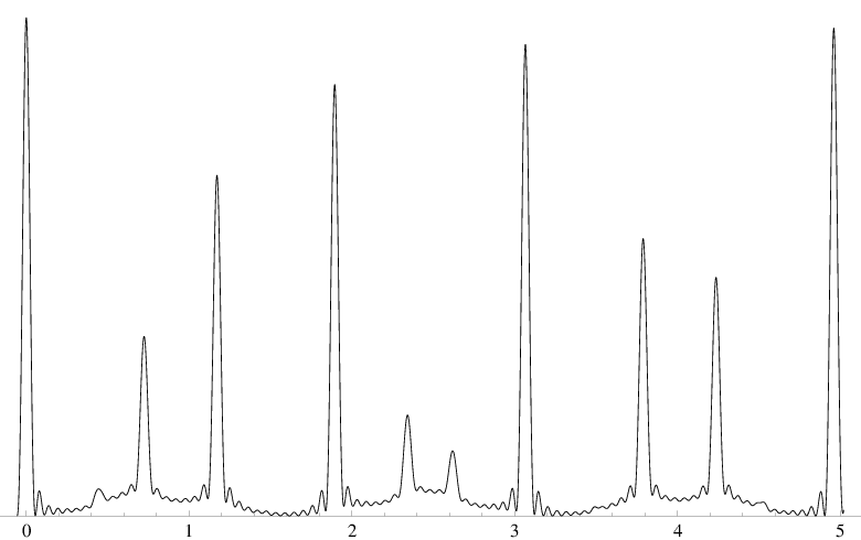
The illustration of an approximation of the diffraction measure $\widehat{\gamma}$ in case of $m=1$ and $p_{0}=p_{1}=\frac{1}{2}$, based on the sequences $A_{n}(k)$ and $B_{n}(k)$, is shown in Figure 1, which agrees with the average over many realisations for the same length.