Anelastic dynamo models with variable electrical conductivity: an application to gas giants
Abstract
The observed surface dynamics of Jupiter and Saturn are dominated by a banded system of fierce zonal winds. The depth of these winds remains unclear but they are thought to be confined to the very outer envelopes where hydrogen remains molecular and the electrical conductivity is small. The dynamo maintaining the dipole-dominated magnetic fields of both gas giants, on the other hand, likely operates in the deeper interior where hydrogen assumes a metallic state.
Here, we present numerical simulations that attempt to model both the zonal winds and the interior dynamo action in an integrated approach. Using the anelastic version of the MHD code MagIC, we explore the effects of density stratification and radial electrical conductivity variations. The electrical conductivity is mostly assumed to remain constant in the thicker inner metallic region and it decays exponentially towards the outer boundary throughout the molecular envelope.
Our results show that the combination of a stronger density stratification and a weaker conducting outer layer is essential for reconciling dipole dominated dynamo action and a fierce equatorial zonal jet. Previous simulations with homogeneous electrical conductivity show that both are mutually exclusive, with solutions either having strong zonal winds and multipolar magnetic fields or weak zonal winds and dipole-dominated magnetic fields. All jets tend to be geostrophic and therefore reach right through the convective shell in our simulations.
The particular setup explored here allows a strong equatorial jet to remain confined to the weaker conducting outer region where it does not interfere with the deeper seated dynamo action. The flanking mid to high latitude jets, on the other hand, have to remain faint to yield a strongly dipolar magnetic field. The fiercer jets on Jupiter and Saturn only seem compatible with the observed dipolar fields when they remain confined to a weaker conducting outer layer.
Keywords:
Atmospheres, dynamics , Jupiter, interior , Variable electrical conductivity , Numerical dynamos1 Introduction
The gas giants, Jupiter and Saturn, mainly consist of a hydrogen-helium mixture. Due to the large pressures and temperatures reached inside these planets, hydrogen acquires metallic properties (Chabrier et al., 1992; Fortney and Nettelmann, 2010). The transition happens at 85–90% of Jupiter’s and % of Saturn’s radii. A classical view is that the lower metallic layer likely hosts the dynamo of these planets, while the upper molecular envelope accommodates the observed fierce zonal jets. Higher densities, Lorentz forces and Ohmic diffusion would lead to a more sluggish dynamics in the metallic layer and confine the zonal winds to the upper region. Traditional dynamical models therefore treat the two layers separately with dynamo simulations modelling only the metallic layer and jet simulations concentrating on the molecular envelope.
The zonal jets have been investigated since the 70s by tracking cloud features (see, for example, Ingersoll et al., 1979 for Jupiter and Sanchez Lavega, 1982 for Saturn). Their driving forces and depth are still debated. Some authors argue that they are a shallow weather phenomenon (Williams, 1978; Cho and Polvani, 1996) while others promote deeper-rooted jets that extend through the whole molecular envelope (Heimpel et al., 2005; Jones and Kuzanyan, 2009; Gastine and Wicht, 2012). Both gas giants emit roughly twice as much energy as they receive from the sun which implies vigorous interior convection. In the rotationally-dominated dynamics ruling planetary atmospheres, interior convection naturally drives zonal winds via Reynolds stresses (Christensen, 2002; Heimpel et al., 2005, i.e. a statistical correlation between the convective flow components;). These winds follow a geostrophic structure, minimizing variations in the direction of the rotation axis, and therefore reach through the whole fluid atmosphere. Lian and Showman (2008) show that even when the forcing is restricted to a shallow weather layer the jets may reach much deeper into the planet. Kaspi et al. (2009), on the other hand, present an anelastic deep convection model where the equatorial zonal flow is geostrophic and the higher latitude jets are confined to the outer few percent in radius.
Saturn’s magnetic field is very axisymmetric and strongly concentrated at higher latitudes (Cao et al., 2012) which is incompatible with the results of a classical Earth-like dynamo model. A stably stratified layer at the top of the dynamo region (Christensen and Wicht, 2008; Stanley, 2010) or a completely different dynamo driven by differential rotation (Cao et al., 2012) are two proposed alternatives for the special situation encountered at Saturn.
Here we concentrate on Jupiter whose field is very similar to the geomagnetic field so that the well-explored geodynamo models also seem to apply at first sight. These models typically adopt the Boussinesq approximation where the mild % density stratification of Earth’s core is simply ignored. In Jupiter, however, the density increases by more than a factor of 5000 below the bar level. While the stratification is mostly concentrated in the outer molecular envelope, the density still rises by about one order of magnitude across the metallic layer (French et al., 2012, Fig. 1 of). Some newer numerical models therefore use the anelastic approximation which allows to incorporate the effects of the background density stratification while filtering out fast sound waves (Gilman and Glatzmaier, 1981; Stanley and Glatzmaier, 2010; Jones and Kuzanyan, 2009).
In an extensive parameter study, Gastine et al. (2012) (hereafter referred to as GDW12) show that dipole-dominated dynamos are rather rare when stronger stratifications are assumed. GDW12 quantify the stratification in their anelastic models in terms of the number of density scale heights , where and are the densities at the inner and outer boundaries of the simulated shell, respectively. For the larger density stratifications , a value that corresponds to an increase by a factor , no dipole-dominated solutions were found. This is attributed to the fact that the focus of convective action moves progressively outward in cylindrical radius when the stratification is intensified. Once the convective columns are mainly confined to a relatively thin outer shell, a non-axisymmetric dynamo mode is preferred that has previously only been observed in mean field dynamo simulations (Rüdiger et al., 2003; Jiang and Wang, 2006). We will refer to this as the thin-shell dynamo model in the following.
For the smaller to intermediate stratifications , GDW12 find dipole dominated magnetic fields when the local Rossby number remains smaller than a critical value of . This is consistent with the findings of Christensen and Aubert (2006) who introduced as a measure for the relative importance of inertia in their Boussinesq models (see Eq. 21). Multipolar solutions with weaker magnetic fields on the other hand exist for all values which means that both types of solutions coexist below for identical model parameters, forming two distinct branches. This so-called bistability can be attributed to the fact that free-slip boundary conditions were employed (Simitev and Busse, 2009; Schrinner et al., 2012; Gastine et al., 2012). These conditions allow strong zonal winds to develop that compete with large scale magnetic fields. On the dipolar branch, zonal winds are weak, on the multipolar branch they are stronger. When no-slip conditions are used zonal flows generally remain weaker and only the dipolar branch is found for (Christensen and Aubert, 2006).
Ab initio calculations suggest that there is actually no clear phase transition between the regions of molecular and metallic hydrogen states (Lorenzen et al., 2011; French et al., 2012). In the dynamo context, the electrical conductivity profile is of particular importance. Due to the increasing degree of hydrogen ionization, the conductivity rises super-exponentially with depth and matches the conductivity of the metallic region at the transition radius without any pronounced jump. The classical separation of the dynamics for the two envelopes thus becomes questionable. Liu et al. (2008) argue that this has important consequences for the depth of the zonal winds which should remain confined to a shallow outer layer where the conductivity remains negligible. The strong shear associated with the zonal winds would otherwise create strong azimuthal magnetic field and lead to Ohmic heating incompatible with the observed luminosity (Glatzmaier, 2008, see however).
Stanley and Glatzmaier (2010) present an anelastic simulation of a relatively thin shell with exponentially decaying electrical conductivity to model the very outer part of the shell. The model uses extreme parameters (i.e. low Ekman and Prandtl number and high Rayleigh number) and a dipole-dominated magnetic field develops in the presence of strong geostrophic zonal winds. However, since a detailed discussion and a systematic parameter study are missing, it remains impossible to disentangle the effects of density stratification, varying conductivity, and the particular parameter choice. Gómez-Pérez et al. (2010) and Heimpel and Gómez-Pérez (2011) also include a radial conductivity profile in their deep shell Boussinesq models, with a constant conductivity in the deeper interior and an exponential decay in the outer part. These models also demonstrate that well-pronounced deep-rooted zonal winds can be compatible with dipole-dominated dynamo action.
The present paper extends the work of GDW12 by adding an electrical conductivity profile loosely based on the ab initio calculations by French et al. (2012). Following Gómez-Pérez et al. (2010) and Heimpel and Gómez-Pérez (2011), the electrical conductivity profile assumes a constant value in the metallic region and an exponential decay in the molecular region. The aim is to systematically explore under which circumstances dipole-dominated dynamo action and strong zonal surface winds can coexist in anelastic dynamo models.
We describe our model in section 2 with special attention to the anelastic formulation and the electrical conductivity profile. The numerical results are presented in section 3, first concentrating on the question of dipole-dominance and then on the dynamo mechanism. Section 4 summarizes our main results and discusses their implications for the gas giants.
2 Model
2.1 Anelastic approximation
The fluid and convective interior of the planet is modelled by solving the MHD equations in a rapidly-rotating spherical shell. Previous models typically used the Boussinesq approximation, which neglects the background density and temperature variations. This is questionable in gas planets and, following Gilman and Glatzmaier (1981), Braginsky and Roberts (1995) and Lantz and Fan (1999), we therefore adopt the anelastic approximation. This allows to include background variations while ruling out sound waves by neglecting fast local density variations.
We solve the equations in a dimensionless form (Christensen and Aubert, 2006, e.g.), using the shell thickness as a length scale and the viscous diffusion time as a timescale. Here, and are the outer and inner radii, respectively, and is the kinematic viscosity. Temperature and density are both non-dimensionalized by their values at the outer boundary, and . We employ constant entropy boundary conditions and use the imposed contrast across the shell as the entropy scale. There are no internal heat sources and all the heating coming into the shell via the inner boundary leaves it through the outer. While this is not the most realistic heating mode for gas giants, it has been chosen to ease the comparisons with more classical Boussinesq simulations. The magnetic field is scaled by , where is the rotation rate of the shell and is the inner boundary reference value of the magnetic diffusivity . Here, is the magnetic permeability and is the prescribed electrical conductivity profile. Below we will also use the normalized magnetic diffusivity and electrical conductivity profiles related via: .
The medium is assumed to be an electrically conducting ideal polytropic gas. Generally, dynamo simulations solve for small variations around an adiabatic hydrostatic background state that we mark with a tilde in the following. The background temperature profile is then defined by the background temperature gradient and the density profile by , where is the polytropic index. For simplicity, we adopt a gravity profile proportional to radius which implicitly assumes a homogeneous density. The other extreme is to assume that all the mass is concentrated in the centre, which leads to a gravity profile proportional to (Gilman and Glatzmaier, 1981; Jones et al., 2011). GDW12 show that both gravity profiles lead to very similar results. The true profile of the gas giants lies somewhere in-between. The temperature reference state is then given by
| (1) |
where
| (2) |
is the number of density scale heights between the inner and the outer boundaries of the shell and is the ratio between the corresponding radii (see Jones et al., 2011; Gastine and Wicht, 2012, for the full derivation of the reference state).
The dimensionless form of the anelastic equations is
| (3) |
| (4) |
| (5) |
| (6) |
| (7) |
The traceless rate-of-strain tensor S for the homogeneous kinematic viscosity assumed here is given by
| (8) |
where is the identity matrix. The viscous and ohmic heating contributions are
| (9) |
and
| (10) |
The system of Eqs. (3–7) is governed by the dimensionless Ekman number , Rayleigh number , Prandtl number and magnetic Prandtl number at the inner boundary :
| (11) |
| (12) |
| (13) |
| (14) |
The specific heat , the thermal diffusivity , magnetic diffusivity and kinematic viscosity are all assumed to be homogeneous. To quantify gravity we use the reference value at the outer boundary.
2.2 Variable conductivity
To simulate the variable electrical conductivity of hydrogen in the interior of Jupiter, we employ a profile that corresponds to a constant conductivity in the metallic hydrogen layer and an exponential decay in the outer molecular envelope. Both branches are matched via a polynomial that also ensures that the first radial derivative is continuous:
| (15) |
The exponential decay with a rate starts at a radius where the normalized conductivity has already decreased from to . For convenience we also define the relative transition radius in percentage: .
This profile has first been used by Gómez-Pérez et al. (2010) and it seems a fair first approximation to the results from ab initio calculations by French et al. (2012). The super-exponential increase of electrical conductivity over the molecular layer is not feasible to model numerically (see Fig. 1). We thus mainly use a rate of for our simulations, but we also tested in a few cases (see Tab. 2) and for one case with a different (grey profile in Fig. 1, discussed in section 3.2). In all the other cases, was fixed to and was varied assuming values of , , and %. Corresponding simulations for homogeneous conductivity with can be found in GDW12.
2.3 Numerical model
For the numerical simulation of the model described above, we use the anelastic version of the MagIC code (Wicht, 2002; Gastine and Wicht, 2012). This is a pseudo-spectral code that solves Eqs. (3–7) in a spherical shell using a poloidal/toroidal decomposition of the vector fields and :
| (16) |
For the spectral representation of the dependence on latitude and longitude , the poloidal potentials and , the toroidal potentials and , the entropy and the pressure are expanded in spherical harmonic functions up to degree and order . Chebyshev polynomials up to degree are used in the radial direction.
For the parameter studies presented here, we use different resolutions, because the higher gradient in density and electrical conductivity demand an increase of both radial and horizontal resolutions. For the Chebyshev polynomial truncations between and are used while ranges between and . Each simulation is run for at least one magnetic diffusion time with the exception of some cases at the lower Ekman number (see Tab. 2).
Regarding the velocity boundary conditions, we apply a no-slip condition at the inner core boundary and a free-slip condition at the outer boundary in most of our simulations which seems appropriate for a gas planet with a rocky core. A few test cases with no-slip conditions at both boundaries allow to explore the impact of the boundary condition on the dynamics.
The existence of an inner core in Jupiter and its possible size is still unclear. Here, we assume a small and electrically conducting solid inner core with . GDW12 explore and in very similar models with homogeneous electrical conductivity and find generally very similar results.
Furthermore, we use constant entropy boundary conditions and match the magnetic field to a diffusive solution at the inner boundary and to a potential field at the outer boundary. The Ekman number is either or . The larger value allows a more extensive scan of the other system parameters like Rayleigh number, density stratification and electrical conductivity transition radius . At , we could only afford to run eleven cases in a more restricted parameter regime. We assume a Prandtl number of and an inner boundary magnetic Prandtl of typically for and for . Nine additional cases with at and at have also been computed.
| 0.0 | 4 | ||
|---|---|---|---|
| 1.0 | 5 | ||
| 2.0 | 6 | ||
| 3.0 | 43 | ||
| 4.0 | 49 | ||
| 5.0 | 55 | ||
| 5.5 | 58 | ||
| 0.0 | 7 | ||
| 1.0 | 9 | ||
| 2.0 | 11 | ||
| 3.0 | 108 |
All together, we ran 74 cases with Rayleigh numbers between and times supercritical. Gastine and Wicht (2012) examine anelastic convection for an aspect ratio of and show that the critical Rayleigh number increases with increasing stratification . Table 1 demonstrates that we observe a similar trend for the smaller aspect ratio employed here. At a certain stratification, the critical wave number jumps from lower to high values. This is the point where the centre of the flow convection moves from close to the inner to close the outer boundary. The respective transition happens at larger stratifications when the Ekman number is decreased (Jones et al., 2009, see also).
In our anelastic simulations, we consider a polytropic index of and we explore density scale heights ranging from the Boussinesq case to , where the latter corresponds to a density jump of . While ab initio simulations suggest a Jovian stratification of from the bottom of the molecular hydrogen layer to the bar level (Guillot, 1999; French et al., 2012). However, since the density gradient rapidly steepens with radius in the planets outer shell our largest stratifications already cover the inner 99% of Jupiter’s radius.
2.4 Diagnostic parameters
The parameters of all numerical experiments discussed here are listed in Tab. 2 along with several diagnostic quantities that characterize the solution and are defined in the following. The amplitude of the zonal flow contribution is measured in terms of the Rossby number :
| (17) |
where is the rms volume-averaged flow velocity and the triangular brackets denote the angular average
| (18) |
is the axisymmetric azimuthal flow component, and is the volume of the spherical shell. Overbars correspond to azimuthal averages. We use the relative kinetic energy
| (19) |
to quantify the relative importance of zonal flows.
The magnetic Reynolds number estimates the ratio of magnetic field production and diffusion and we use a modified form here to account for the radial-dependent magnetic diffusivity:
| (20) |
The local Rossby number has been introduced by Christensen and Aubert (2006) to quantify the relative importance of the advection term in the Navier-Stokes equation (Eq. 3) and is defined as
| (21) |
Here, is a typical flow length scale given by
| (22) |
where is the flow contribution of spherical harmonic degree . We use a modified form of based exclusively on the inner conducting region ():
| (23) |
The magnetic field strength is quantified by the Elsasser number which measures the ratio of Lorentz to Coriolis forces using the modified form
| (24) |
The geometry of the surface field is characterized by the dipolarity
| (25) |
which measures the relative energy in the axial dipole contribution at the outer boundary . Following Christensen and Aubert (2006), we restricted the magnetic field to spherical harmonic degrees and orders below 12 in Eq. (25). Tab. 2 lists time averages of the properties defined above for all our models and we always refer to the time-averaged properties for characterizing our solutions in the following. The time variability of the dipolarity, also listed in Tab. 2, is quantified by its standard deviation .
3 Results
3.1 Dynamo regimes
In the complex models explored here, the magnetic field geometry not only depends on the local Rossby number (Christensen and Aubert, 2006) but also on the density stratification, on the thickness of the weaker conducting layer, on the Ekman number, and on the magnetic Prandtl number. Fig. 2 shows the dependence of the dipolarity on the local Rossby number for all our cases, excluding runs with , with the exception of case 67 from Tab. 2 which is similar to one of Heimpel and Gómez-Pérez (2011)’s runs. To illustrate the relation between the field geometry and the zonal flows, we plot versus the relative kinetic energy of axisymmetric azimuthal flows in Fig. 3. In both figures, the symbol type refers to the different stratifications while the symbol colour identifies the four transitional radii explored here. We start by analysing the different dynamo regimes based on the results for and and come back to the solutions for larger magnetic Prandtl numbers and for further below.
When the weakly conducting layer is relatively thin ( and ) and the stratification is mild to intermediate , we find two distinct branches. A dipolar branch, characterized by and weak zonal flows, is restricted to cases with local Rossby numbers below the critical value of . This is significantly lower than the values of suggested for homogeneous electrical conductivity by GDW12. The dipole-dominated solutions forming this branch are located in the upper left corner of Fig. 2 and in the left portion of the yellow high-dipolarity regime in Fig. 3.
A second branch with multipolar magnetic fields at but intermediate zonal flows exists for all values. These solutions can be found in the lower part of Fig. 2 and the cyan low-dipolarity regime in Fig. 3.
For local Rossby numbers below , we thus find both types of solutions while only multipolar solutions remain stable beyond . Figures 2 and 3 contain seven examples (dashed lines) where a solution on each branch is found for identical model parameters, clearly demonstrating the bistability for . Which branch a specific numerical simulation will chose depends on the initial magnetic field configuration. Note that the multipolar attractor always has the more intense zonal flows (see Fig. 3). Comparing magnetic Reynolds numbers and local Rossby numbers for bistable cases shows that the relative difference is smaller in the latter than in the former measure. This indicates that the weaker flow amplitude caused by the larger Lorentz forces in the dipole-dominated cases is accompanied by a growth in the flow length scale.
Increasing the stratification to values beyond while keeping large always leads to solutions of the multipolar thin-shell type discussed by GDW12. Altogether, the behaviour for a thin weakly conducting layer is similar to that for a homogeneous electrical conductivity with the exception of the lower critical Rossby number .
For a thicker weakly conducting layer with %, the influence of the stratification on the dipolarity is reversed. Clearly, dipolar solutions with now exclusively exist for stratifications of or . Since the relative zonal flow amplitude reaches intermediate values, these cases can be found in the middle section of the yellow regime in Fig. 3. A second branch of solutions is characterized by low to intermediate dipolarity that increases with and by large relative zonal flow amplitudes. These cases populate the pink region in Fig. 3. For stratification of , the solutions on this secondary branch become strongly time-dependent as indicated by the large error bars in Figs. 2 and 3. Figure 4 demonstrates that the time dependence reflects an oscillation between dipolar and multipolar field configurations without ever establishing a solution on the dipole-dominated branch. Polarity reversals or excursions become possible when the dipolarity is relatively low.
Once more, both branches coexist for not too large local Rossby numbers and we could identify two bistable cases for %, and , . When increasing the Rayleigh number to , however, only the multipolar solution remains which suggests a critical local Rossby number of about (see Tab. 2).
For %, the thickest weakly conducting outer shell explored here, even stronger stratification seems required to establish a dipole dominated magnetic field than at %. For the magnetic Prandtl number , generally used at , only the highly time-dependent solutions with intermediate dipolarity and strong zonal winds (on average) were found, even at . However, the mean dipolarity increases with , just as in the % cases and stratifications of may finally establish a dipole-dominated solution.
Figure 5 highlights the role of the density stratification at %, %, % and % for models at and with similar local Rossby numbers. When the weakly conducting layer is relatively thin ( or ), dipole-dominated solutions can only be found for while multipolar solutions exist for all stratifications. For a thicker layer, however, the stratification has a reversed effect. The mean dipolarity increases with stratification and highly dipolar solutions are only found for stronger stratifications . Note that at % and , we could only find multipolar solutions, even at low Rayleigh numbers where is small. The reason for this is not yet understood. What finally helped to establish a dipolar solution here was increasing the magnetic Prandtl number from to .
We also tested the effect of larger magnetic Prandtl numbers for several other parameter combinations and this often promoted dipole-dominated solutions. For example, at % and a multipolar case became dipolar when increasing from to . Likewise, the highly time-dependent case at %, , and developed into a stable dipole-dominated solution when doubling . The same behaviour was found at %, and . This indicates a certain trade-off between larger stratifications and higher electrical conductivities. At % or %, and , however, an increase from to was not sufficient to establish a dipole-dominated solution. Even higher magnetic Prandtl numbers may be required here.
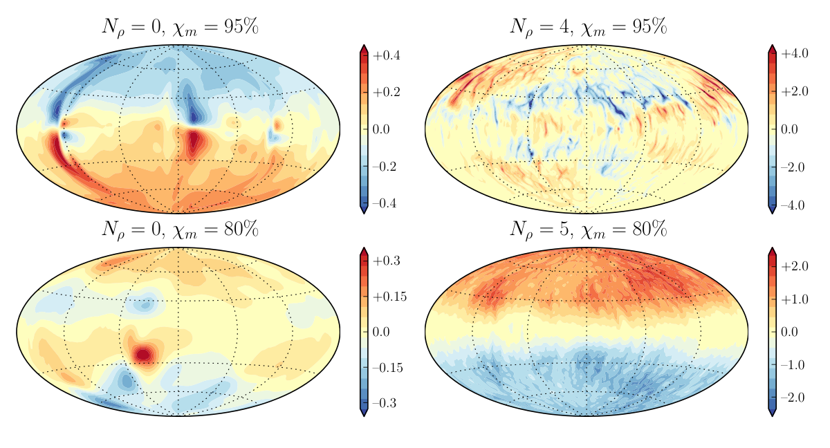
Figure 6 illustrates the different types of solutions with snapshots of the radial magnetic field at the outer boundary for . The top row shows cases at two different stratifications: a dipole-dominated Boussinesq case and a multipolar solution at . The latter shows a large scale wave number () structure similar to that reported for multipolar dynamos with homogeneous electrical conductivity and free-slip boundaries (Goudard and Dormy, 2008, GDW12). The bottom row of Fig. 6 depicts the two branches found for . The left panel shows a snapshot of a Boussinesq multipolar case and the right panel illustrates the dipolar configuration found at strong stratifications ().
The results by Heimpel and Gómez-Pérez (2011) prompted us to also conduct simulations at the lower Ekman number of used in their study. Tab. 2 lists the respective models with different Rayleigh numbers and stratifications. The thicker weakly conducting layer of % was generally chosen except for one model with %. The Boussinesq case 67 is identical to one of the models presented by Heimpel and Gómez-Pérez (2011) and has a larger aspect ratio of instead of . The outer grey line of the symbols in Figs. 2 and 3 corresponds to the twelve runs with .
While for and % we had to increase the stratification to to find strongly dipolar solutions, this is not the case any more at . Even the Boussinesq models now clearly have dipole-dominated magnetic fields. The only multipolar case, which seems to be of the highly time-dependent type, is found at and it has a local Rossby number of . Another model at but is strongly dipolar so that the critical local Rossby number can be estimated to . Note however, that may depend on stratification.
3.2 The role of zonal flows
The coexistence of dipolar and multipolar branches indicates a competition between zonal winds and dipolar magnetic fields already discussed by GDW12. The stronger Lorentz forces associated to the larger dipolar fields effectively compete with the Reynolds stresses responsible for driving the zonal winds. The zonal wind amplitude and the relative zonal wind energy thus remain typically small. Fierce zonal winds, on the other hand, seem to promote multipolar fields. This is at least the situation for and % or %. But why are stronger stratifications and/or larger magnetic Prandtl numbers required to yield dipole-dominated dynamo action for thicker weakly conducting outer layers?

Figure 7 illustrates the zonal flow structure and the poloidal magnetic field lines for different stratifications at % (middle row) and % (bottom row) for . The top row shows non-magnetic cases and demonstrates that the inner retrograde jet decreases in amplitude when the stratification intensifies. This reflects the progressive outward concentration of the convective motions and thus of the Reynolds stresses driving the zonal flows (GDW12).
The dominance of Coriolis forces at this relatively low Ekman number enforces the Taylor-Proudman theorem and the intense zonal jets remain strongly geostrophic, i.e. variations in the direction of the rotation axis are much smaller than variations perpendicular to it. For the thinner weakly conducting layer (middle row in Fig. 7), the Lorentz forces associated with the stronger dipolar field at mild stratifications effectively suppress the zonal flows in the whole shell. For , the weaker multipolar fields created by the thin-shell dynamo allow the outer prograde jet to survive, albeit with a significantly reduced amplitude and a restricted width than in the non-magnetic simulations. The thickness of the weakly conducting layer now determines the width of the outer jet, confirming previous work by Heimpel and Gómez-Pérez (2011).
At % (lower row in Fig. 7), the zonal flows generally remain more energetic than for %. Since these flows are largely geostrophic, the force balances on geostrophic cylinders (i.e. on cylinders aligned with the rotation axis) should be considered. The Lorentz forces now have a harder time to brake the zonal flows since they act in a significantly reduced volume. Dipole-dominated dynamo action only becomes possible when the retrograde inner zonal jet is already relatively weak in the non-magnetic simulations, which happens at stronger stratifications. The thin-shell dynamo mechanism generating the multipolar field for % does not apply here, since it would have to operate, at least partly, in the weakly conducting layer where the magnetic Reynolds number is now too low to support dynamo action. Instead, a strongly dipolar magnetic field is generated in the deeper interior where it does not interfere with the remaining prograde outer zonal jet.
The change in the depth of the poloidal dynamo action is further illustrated by the radial profiles of magnetic energy shown in Fig. 8. Up to a stratification of , poloidal and toroidal magnetic energies have similar profiles and peak in the outer part of the conducting region around . For , however, the profiles are different with a pronounced focus on deeper parts of the shell around . For , the toroidal magnetic field is larger than the poloidal, suggesting that the induction mechanism is different from the dipole-dominated case at where the poloidal field is stronger.
At %, the volume over which Lorentz forces can efficiently brake zonal winds is even further reduced. Dipolar solutions can only be found at even larger stratification than at % where the driving of the inner zonal jet is yet weaker.
The role of Lorentz forces in defeating zonal winds and thereby enabling dipole-dominated magnetic fields also offers an explanation why larger magnetic Prandtl numbers help. The reason likely is that larger values lead to stronger magnetic fields and thus stronger Lorentz forces. We can also now interpret the highly time-dependent solutions with intermediate mean dipolarities. Here, the balance seems to be undecided (Fig. 4). Stronger Lorentz forces successfully suppress the zonal winds at times but never enough to establish the solution on the highly dipolar more stable branch. At other times, Reynolds stresses succeed in driving stronger zonal flows that mostly create a weaker multipolar magnetic field.
To further test the theory that the zonal flows are decisive for the field geometry we ran a few cases with a no-slip outer boundary condition that largely prevents zonal flows from developing. The results are mixed and not entirely conclusive, which may have to do with the fact that other flow components are also affected by this change in boundary conditions. At %, and , the no-slip boundary conditions indeed promote a dipole-dominated solution with weak zonal flows where we only find multipolar solutions with strong zonal flows for a free-slip outer boundary condition (compare cases 3 and ). The same positive effect was found for %, and (cases 7 and ). At %, and , however, we find bistable cases for both type of boundary conditions (cases 22d/m and d/m). In the no-slip case, both the dipole-dominated and the multipolar solution have weak zonal flows. Free-slip outer boundary condition promotes dipolarity, but it is not a necessary condition to find this feature. Note that such a bistable case for no-slip conditions has already been reported by Christensen and Aubert (2006).
At %, and , the suppression of the zonal flows by the no-slip condition is not sufficient to yield a dipole-dominated solution and the same is true at %, and or (cases 17, 32 and 36). In the latter two examples, the particular thin shell dynamo described by GDW12, rather than the stronger zonal flows, may be the reason for the multipolarity which could explain why the no-slip condition has no effect.
We also varied the electrical conductivity profile in a few cases. Increasing the exponential decay rate from to for two simulations at % required a finer radial numerical grid and thus more expensive numerical simulations. The zonal flows in the weakly conducting layer were intensified in both cases, likely because of the further decreased weaker Lorentz forces there. The type of solution, however, remained unchanged (see cases 33/34 and 51/52).
We also tested a more realistic profile that models the approximately linear decrease of electrical conductivity in the metallic layer (see Fig. 1) and a steeper decrease at larger radii. At %, and the solution is bistable for our standard conductivity profile. For the more realistic profile we so far only found a clearly dipole-dominated at the same supercriticality but we cannot exclude that the multipolar case also exists. Figure 9 compares the radial profiles of the convective magnetic Reynolds number for both profiles (yellow lines and grey line). Being based on rms flows velocities that exclude zonal winds, is appropriate for characterizing poloidal magnetic field production. Numerical simulations suggest that a magnetic Reynolds number larger than is required to support dynamo action (Christensen and Aubert, 2006). For our standard electrical conductivity profiles, typically falls below this value for radii beyond or . The linear decrease in the metallic layer, however, further reduces the convective Reynolds number which is already very low at depth. values larger than are now restricted to the inner region of . A multipolar dynamo where the outer parts of the shell play a sizeable role thus becomes unlikely. In Jupiter, is generally significantly higher in the metallic region and only decreases below the critical value for dynamo action in the molecular envelope. We therefore refrained from further exploring this profile since the decrease in magnetic Reynolds number artificially limits the dynamo region.
Figure 10 shows zonal flows and axisymmetric poloidal field lines for the dipole-dominated solutions at with the modified electrical conductivity profile (first panel from the left) and the standard profile (second panel). The poloidal fields are very similar and produced at greater depth in both cases. This explains why the low convective magnetic Reynolds number in the outer part of the shell has little impact on the dynamo mechanism for dipolar dominated solutions. Once more, the weaker Lorentz force in the outer layer allows for more vigorous zonal winds for the more realistic conductivity profile.
How do the results at fit into the picture we outlined above? Figure 10 compares two cases at (third panel, case 60) and (fourth panel, case 66) with the dipole-dominated solutions for the more realistic profile (first panel, case 50) and for our standard profile at and (second panel, case 51, see also Fig. 7). The magnetic field and zonal flow structures are very similar in all cases. At both Ekman numbers, the relative amplitude of the retrograde jets decreases with increasing (see also Tab. 2). The absolute zonal flow amplitude, however, is significantly smaller in all lower Ekman number models. For example, the zonal flow Rossby number is in the / case (66) depicted in Fig. 10, but in the / simulation (51).
In non-magnetic free-slip simulations, the flow amplitude roughly scales with the modified Rayleigh number , as it has been shown by Christensen (2002) for Boussinesq and Gastine and Wicht (2012) for anelastic models. For example, Gastine and Wicht (2012) suggest the dependence . This scaling describes an asymptotic behaviour for larger Rayleigh numbers where zonal flows clearly dominate so that . For the smaller Rayleigh numbers typically examined here, it may only serve as a rough estimate for the zonal flow amplitude. For case 51 with , we have and the scaling predicts . For case 66 with and , it predicts . Both values are not too far from the numerical results and , respectively, which suggests that the difference in is indeed the main reason for the much weaker zonal flows at the lower Ekman number.
Because of the quadratic Ekman number dependence of , has to be increased by two orders of magnitude to reach the same zonal flow amplitudes in the as in the cases. This leads to larger values and thus possibly multipolar fields (Heimpel and Gómez-Pérez, 2011). The Rayleigh number increase from (case 61) to (case 62) at already leads to a multipolar field while only doubling the zonal flow amplitude.
The similar Elsasser numbers in the dipole-dominated cases at both Ekman numbers indicate that the Lorentz forces also have comparable amplitudes. These forces have a much easier job to brake the systematically weak zonal flows at , allowing a dipole-dominated field to develop even at mild stratifications. The more extensive parameter study at suggests that stronger stratifications should allow for more vigorous outer jets while retaining dipole-dominated dynamo action.
3.3 Dynamo Mechanism
GDW12 reported that the multipolar solutions with stronger zonal flows are dynamos of an or an type. Dynamos of the type, on the other hand, are known to produce dipole-dominated magnetic fields (Olson et al., 1999). The stands for poloidal and toroidal field production by local helical structures, while stands for the production of toroidal field by global zonal wind shear. Following Brown et al. (2011), the -effect is given by
| (26) |
and describes the production of the axisymmetric azimuthal magnetic field which is purely toroidal. The mean ohmic diffusion of is given by
| (27) |

Figure 11 compares , and MD for two % cases, a multipolar solution at (left) and dipole dominated solution at (right). Both cases were depicted previously in Figs. 7 and 8. For the multipolar solution, the -effect plays an important role, as demonstrated by the high degree of correlation with the azimuthal field over the shell. For the dipole-dominated solution, however, the -effect is only strong in the weakly conducting region where it is effectively balanced by the large ohmic diffusion. The change in field geometry is thus once more coupled to a switch from an or mechanism at weaker stratifications to an mechanism at stronger density stratifications.
4 Conclusions
We ran a suite of dynamo simulations with an electrical conductivity profile geared to combine the dynamics of the metallic and the molecular hydrogen layers of the gas giants in one integrated model. In most models, the conductivity is assumed to remain constant over the inner part of the shell representing the metallic hydrogen region. Beyond a relative radius of , it decays exponentially with radius, to model the molecular envelope. The use of the anelastic MHD code allowed us to also study the effects of density stratification. Free-slip outer boundary and no-slip inner boundary conditions seem appropriate for the gas giants and were used in the majority of our simulations.
In GDW12, we had explored the dynamo action for homogeneous electrical conductivity in an otherwise identical setup. Dipole-dominated solutions were only found for mild stratifications and local Rossby numbers below . The respective solution branch is characterized by weak zonal winds and coexists with a second branch with weaker multipolar magnetic fields but stronger zonal winds at identical parameters. This indicates a competition between zonal winds and dipolar magnetic fields (Simitev and Busse, 2009; Schrinner et al., 2012; Gastine et al., 2012). Translated to Jupiter and Saturn, these simulations would predict multipolar magnetic fields, should the observed zonal winds reach into the dynamo region. The strong stratification within the gas giants should also promote multipolar solutions.
We largely recover these results when the outer weakly conducting layer occupies only or percent in radius ( and ). However, the critical local Rossby number, below which dipole-dominated solutions are possible, decreases to . Gómez-Pérez et al. (2010) already showed that even very thin weakly conducting outer layers promote multipolar magnetic field configurations. They speculate that the separation of the Ekman and Hartmann boundary layers may play a role in their models with no-slip boundaries, although this explanation is difficult to apply for the free-slip models predominantly explored here. More research is required to clarify this point in the future, specially concerning no-slip boundaries.
For a thicker weakly conducting outer layer covering the outer 20 or 30% in radius (% or %), the volume over which the Lorentz forces can act to balance Reynolds stresses is more significantly reduced. The competition between zonal wind and stronger dipolar fields thus becomes even more of an issue. At an Ekman number of , the mean zonal winds tend to be relatively strong even at low Rayleigh numbers. Dipole-dominated dynamo action is nevertheless possible in the deeper interior of strongly stratified models, where the zonal flows remain relatively weak even in the non-magnetic case. Alternatively, dipole-dominated solutions are found for larger magnetic Prandtl numbers which help to keep zonal flows at bay by increasing Lorentz forces. In the dipole-dominated solutions, the zonal winds are then mainly restricted to a fierce prograde jet that resides within the weakly conducting outer envelope.
At the lower Ekman number of , dipole-dominated magnetic fields can even be maintained at weak stratifications because the zonal flow amplitudes are lower than at . The peak velocity of Jupiter’s equatorial jet is around (Vasavada and Showman, 2005) and about for Saturn (Choi et al., 2009). For example, the case illustrated in Fig. 10 (second panel from the left) reaches which is somewhat too high for Jupiter. The simulation depicted in the same figure has at the lower stratification of . The amplitude of the equatorial jet decreases with Ekman number and increases with density stratification. We speculate that the higher stratifications within the gas giants may allow to reach appropriate zonal jet amplitudes at the much lower realistic Ekman number, around (French et al., 2012), while retaining dipole-dominated dynamo action.
The number of zonal jets is much smaller in our simulations than for the gas giants. Also, the strong decrease in the zonal flow amplitude from the equatorial to the flanking jets, that is necessary to retain dipole-dominated dynamo action in our models, is not compatible with the observations for Jupiter. A dipolar configuration nevertheless seems possible should the higher latitude jets remain too shallow to interfere with the deeper dynamo process. The equatorial jet does not pose a problem in this respect because it can reside completely within the lower conductivity envelope.
An argument against deep reaching winds is that the associated strong -effect and Ohmic dissipation may not be compatible with Jupiter’s observed luminosity (Liu et al., 2008). A first analysis of our results confirms that the -effect and associated Ohmic dissipation can be significant. Glatzmaier (2008) argues that the magnetic field may assume a configuration where the poloidal field lines are aligned with the rotation axis in regions of strong zonal flow shear. Since the shear is perpendicular to the rotation axis, this would minimize the -effect and related Ohmic dissipation. Figure 10 illustrates that the field lines indeed approach such an alignment in the very outer part of the shell where the electrical conductivity is still important. The Ohmic dissipation nevertheless remains significant in all our simulations with strong zonal flows. Further investigation is necessary to quantify this effect and extrapolate it to the planetary situation.
Any problems related to ohmic dissipation and dipolar dynamo action would not be an issue when stronger zonal winds remain confined to a thin outer envelope with (), where the electrical conductivity remains small enough (Liu et al., 2008). In our simulations, however, all the stronger jets obey the Taylor-Proudman theorem and reach through the planet. Shallow jets have been found by Kaspi et al. (2009), who use a different anelastic approximation and a different internal heating mode. Further investigations are required to clarify which specific model features influence the depth on the zonal jets.
Acknowledgements
All the computations have been carried out in the GWDG computer facilities in Göttingen, in the Norddeutscher Verbund für Hoch- und Höchstleistungsrechnen (HLRN) in Hannover and in the Max-Planck-Institut für Sonnensystemforschung. The authors would like to specially thank the reviewers and editor for the much helpful comments and suggestions and also HLRN for providing the possibility of carrying out demanding "last minute" simulations that allowed improvement of the work. This work was supported by the Special Priority Program 1488 (PlanetMag, http://www.planetmag.de) of the German Science Foundation.
References
- Braginsky and Roberts (1995) Braginsky, S. I., Roberts, P. H., 1995. Equations governing convection in earth’s core and the geodynamo. Geophysical and Astrophysical Fluid Dynamics 79, 1–97.
- Brown et al. (2011) Brown, B. P., Miesch, M. S., Browning, M. K., Brun, A. S., Toomre, J., Apr. 2011. Magnetic Cycles in a Convective Dynamo Simulation of a Young Solar-type Star. ApJ 731, 69.
- Cao et al. (2012) Cao, H., Russell, C. T., Wicht, J., Christensen, U. C., Dougherty, M. K., Aug. 2012. Saturn’s High Degree Magnetic Moments: Evidence for a Unique Planetary Dynamo. Icarus, in press.
- Chabrier et al. (1992) Chabrier, G., Saumon, D., Hubbard, W. B., Lunine, J. I., Jun. 1992. The molecular-metallic transition of hydrogen and the structure of Jupiter and Saturn. ApJ 391, 817–826.
- Cho and Polvani (1996) Cho, J. Y.-K., Polvani, L. M., Jul. 1996. The Morphogenesis of Bands and Zonal Winds in the Atmospheres on the Giant Outer Planets. Science 273, 335–337.
- Choi et al. (2009) Choi, D. S., Showman, A. P., Brown, R. H., Apr. 2009. Cloud features and zonal wind measurements of Saturn’s atmosphere as observed by Cassini/VIMS. Journal of Geophysical Research (Planets) 114, 4007.
- Christensen (2002) Christensen, U. R., Nov. 2002. Zonal flow driven by strongly supercritical convection in rotating spherical shells. Journal of Fluid Mechanics 470, 115–133.
- Christensen and Aubert (2006) Christensen, U. R., Aubert, J., Jul. 2006. Scaling properties of convection-driven dynamos in rotating spherical shells and application to planetary magnetic fields. Geophysical Journal International 166, 97–114.
- Christensen and Wicht (2008) Christensen, U. R., Wicht, J., Jul. 2008. Models of magnetic field generation in partly stable planetary cores: Applications to Mercury and Saturn. Icarus 196, 16–34.
- Fortney and Nettelmann (2010) Fortney, J. J., Nettelmann, N., May 2010. The Interior Structure, Composition, and Evolution of Giant Planets. Space Sci. Rev. 152, 423–447.
- French et al. (2012) French, M., Becker, A., Lorenzen, W., Nettelmann, N., Bethkenhagen, M., Wicht, J., Redmer, R., Sep. 2012. Ab Initio Simulations for Material Properties along the Jupiter Adiabat. ApJS 202, 5.
- Gastine et al. (2012) Gastine, T., Duarte, L., Wicht, J., Oct. 2012. Dipolar versus multipolar dynamos: the influence of the background density stratification. A&A 546, A19.
- Gastine and Wicht (2012) Gastine, T., Wicht, J., May 2012. Effects of compressibility on driving zonal flow in gas giants. Icarus 219, 428–442.
- Gilman and Glatzmaier (1981) Gilman, P. A., Glatzmaier, G. A., Feb. 1981. Compressible convection in a rotating spherical shell. I - Anelastic equations. II - A linear anelastic model. III - Analytic model for compressible vorticity waves. ApJS 45, 335–388.
- Glatzmaier (2008) Glatzmaier, G. A., Aug. 2008. A note on “Constraints on deep-seated zonal winds inside Jupiter and Saturn”. Icarus 196, 665–666.
- Gómez-Pérez et al. (2010) Gómez-Pérez, N., Heimpel, M., Wicht, J., Jul. 2010. Effects of a radially varying electrical conductivity on 3D numerical dynamos. Physics of the Earth and Planetary Interiors 181, 42–53.
- Goudard and Dormy (2008) Goudard, L., Dormy, E., Sep. 2008. Relations between the dynamo region geometry and the magnetic behavior of stars and planets. EPL (Europhysics Letters) 83, 59001.
- Guillot (1999) Guillot, T., Oct. 1999. Interior of Giant Planets Inside and Outside the Solar System. Science 286, 72–77.
- Heimpel et al. (2005) Heimpel, M., Aurnou, J., Wicht, J., Nov. 2005. Simulation of equatorial and high-latitude jets on Jupiter in a deep convection model. Nature 438, 193–196.
- Heimpel and Gómez-Pérez (2011) Heimpel, M., Gómez-Pérez, N., Jul. 2011. On the relationship between zonal jets and dynamo action in giant planets. Geophys. Res. Lett. 38, 14201.
- Ingersoll et al. (1979) Ingersoll, A. P., Beebe, R. F., Collins, S. A., Mitchell, J. L., Terrile, R. J., Hunt, G. E., Muller, P., Smith, B. A., Aug. 1979. Zonal velocity and texture in the Jovian atmosphere inferred from Voyager images. Nature 280, 773–775.
- Jiang and Wang (2006) Jiang, J., Wang, J.-X., Apr. 2006. A Non-axisymmetric Spherical 2-Dynamo. Chinese J. Astron. Astrophys. 6, 227–236.
- Jones et al. (2011) Jones, C. A., Boronski, P., Brun, A. S., Glatzmaier, G. A., Gastine, T., Miesch, M. S., Wicht, J., Nov. 2011. Anelastic convection-driven dynamo benchmarks. Icarus 216, 120–135.
- Jones and Kuzanyan (2009) Jones, C. A., Kuzanyan, K. M., Nov. 2009. Compressible convection in the deep atmospheres of giant planets. Icarus 204, 227–238.
- Jones et al. (2009) Jones, C. A., Kuzanyan, K. M., Mitchell, R. H., Aug. 2009. Linear theory of compressible convection in rapidly rotating spherical shells, using the anelastic approximation. Journal of Fluid Mechanics 634, 291.
- Kaspi et al. (2009) Kaspi, Y., Flierl, G. R., Showman, A. P., Aug. 2009. The deep wind structure of the giant planets: Results from an anelastic general circulation model. Icarus 202, 525–542.
- Lantz and Fan (1999) Lantz, S. R., Fan, Y., Mar. 1999. Anelastic Magnetohydrodynamic Equations for Modeling Solar and Stellar Convection Zones. ApJS 121, 247–264.
- Lian and Showman (2008) Lian, Y., Showman, A. P., Apr. 2008. Deep jets on gas-giant planets. Icarus 194, 597–615.
- Liu et al. (2008) Liu, J., Goldreich, P. M., Stevenson, D. J., Aug. 2008. Constraints on deep-seated zonal winds inside Jupiter and Saturn. Icarus 196, 653–664.
- Lorenzen et al. (2011) Lorenzen, W., Holst, B., Redmer, R., Dec. 2011. Metallization in hydrogen-helium mixtures. Phys. Rev. B 84 (23), 235109.
- Olson et al. (1999) Olson, P., Christensen, U., Glatzmaier, G. A., May 1999. Numerical modeling of the geodynamo: Mechanisms of field generation and equilibration. J. Geophys. Res. 104, 10383–10404.
- Rüdiger et al. (2003) Rüdiger, G., Elstner, D., Ossendrijver, M., Jul. 2003. Do spherical 2-dynamos oscillate? A&A 406, 15–21.
- Sanchez Lavega (1982) Sanchez Lavega, A., Jan. 1982. Motions in Saturn’s atmosphere - Observations before Voyager encounters. Icarus 49, 1–16.
- Schrinner et al. (2012) Schrinner, M., Petitdemange, L., Dormy, E., Jun. 2012. Dipole Collapse and Dynamo Waves in Global Direct Numerical Simulations. ApJ 752, 121.
- Simitev and Busse (2009) Simitev, R. D., Busse, F. H., Jan. 2009. Bistability and hysteresis of dipolar dynamos generated by turbulent convection in rotating spherical shells. EPL (Europhysics Letters) 85, 19001.
- Stanley (2010) Stanley, S., Mar. 2010. A dynamo model for axisymmetrizing Saturn’s magnetic field. Geophys. Res. Lett. 37, 5201.
- Stanley and Glatzmaier (2010) Stanley, S., Glatzmaier, G. A., May 2010. Dynamo Models for Planets Other Than Earth. Space Sci. Rev. 152, 617–649.
- Vasavada and Showman (2005) Vasavada, A. R., Showman, A. P., Aug. 2005. Jovian atmospheric dynamics: an update after Galileo and Cassini. Reports on Progress in Physics 68, 1935–1996.
- Wicht (2002) Wicht, J., Oct. 2002. Inner-core conductivity in numerical dynamo simulations. Physics of the Earth and Planetary Interiors 132, 281–302.
- Williams (1978) Williams, G. P., Aug. 1978. Planetary circulations. I - Barotropic representation of Jovian and terrestrial turbulence. Journal of Atmospheric Sciences 35, 1399–1426.
| Model | ||||||||||||||
|---|---|---|---|---|---|---|---|---|---|---|---|---|---|---|
| 01d | 95 | 0.0 | 11.5 | 7385 | 0.04 | 130 | ||||||||
| 01m | 95 | 0.0 | 11.5 | 73106 | 0.36 | 157 | ||||||||
| 02 | 95 | 0.0 | 17.2 | 73106 | 0.37 | 236 | ||||||||
| 03 | 95 | 0.0 | 23.0 | 73106 | 0.35 | 290 | ||||||||
| 04∗ | 95 | 0.0 | 23.0 | 73106 | 0.04 | 239 | ||||||||
| 05 | 90 | 0.0 | 9.2 | 6164 | 0.07 | 242 | ||||||||
| 06 | 90 | 0.0 | 10.3 | 7385 | 0.57 | 130 | ||||||||
| 07 | 90 | 0.0 | 11.5 | 73106 | 0.50 | 153 | ||||||||
| 08∗ | 90 | 0.0 | 11.5 | 73106 | 0.04 | 114 | ||||||||
| 09 | 90 | 0.0 | 23.0 | 73106 | 0.38 | 270 | ||||||||
| 10∗ | 90 | 0.0 | 23.0 | 73106 | 0.10 | 241 | ||||||||
| 11 | 80 | 0.0 | 11.5 | 73106 | 0.65 | 140 | ||||||||
| 12 | 80 | 0.0 | 11.5 | 73106 | 0.09 | 403 | ||||||||
| 13∗ | 80 | 0.0 | 11.5 | 73106 | 0.03 | 395 | ||||||||
| 14 | 80 | 0.0 | 17.2 | 73106 | 0.64 | 206 | ||||||||
| 15∗ | 80 | 0.0 | 20.7 | 7385 | 0.11 | 162 | ||||||||
| 16 | 80 | 0.0 | 23.0 | 73106 | 0.62 | 276 | ||||||||
| 17∗ | 80 | 0.0 | 23.0 | 73106 | 0.09 | 177 | ||||||||
| 18 | 80 | 0.0 | 45.9 | 81170 | 0.62 | 454 | ||||||||
| 19d | 95 | 1.0 | 4.1 | 7385 | 0.05 | 90 | ||||||||
| 19m | 95 | 1.0 | 4.1 | 7385 | 0.21 | 103 | ||||||||
| 20d | 95 | 1.0 | 5.2 | 73106 | 0.04 | 121 | ||||||||
| 20m | 95 | 1.0 | 5.2 | 73106 | 0.18 | 145 | ||||||||
| 21 | 95 | 1.0 | 7.8 | 7385 | 0.21 | 234 | ||||||||
| 22d | 90 | 1.0 | 5.2 | 7385 | 0.06 | 103 | ||||||||
| 22m | 90 | 1.0 | 5.2 | 7385 | 0.26 | 126 | ||||||||
| 23d∗ | 90 | 1.0 | 5.2 | 7385 | 0.04 | 110 | ||||||||
| 23m∗ | 90 | 1.0 | 5.2 | 7385 | 0.05 | 131 | ||||||||
| 24 | 90 | 1.0 | 7.8 | 73106 | 0.30 | 204 | ||||||||
| 25 | 80 | 1.0 | 5.2 | 73106 | 0.58 | 95 | ||||||||
| 26 | 80 | 1.0 | 10.3 | 73106 | 0.65 | 224 | ||||||||
| 27 | 95 | 2.0 | 2.9 | 73106 | 0.28 | 107 | ||||||||
| 28 | 95 | 3.0 | 3.2 | 73106 | 0.29 | 158 | ||||||||
| 29 | 90 | 3.0 | 3.2 | 7385 | 0.45 | 124 | ||||||||
| 30 | 80 | 3.0 | 3.2 | 7385 | 0.72 | 76 | ||||||||
| 31 | 80 | 3.0 | 3.2 | 121106 | 0.52 | 215 | ||||||||
| 32∗ | 80 | 3.0 | 3.2 | 73106 | 0.23 | 90 | ||||||||
| 33 | 80 | 3.0 | 4.3 | 73106 | 0.67 | 134 | ||||||||
| 34(1) | 80 | 3.0 | 4.3 | 121106 | 0.71 | 128 | ||||||||
| 35 | 80 | 3.0 | 4.3 | 145106 | 0.45 | 341 | ||||||||
| 36∗ | 80 | 3.0 | 4.3 | 73106 | 0.19 | 137 | ||||||||
| 37 | 80 | 3.0 | 8.6 | 81170 | 0.55 | 258 | ||||||||
| 38 | 70 | 3.0 | 4.3 | 73106 | 0.77 | 90 | ||||||||
| 39 | 70 | 3.0 | 4.3 | 129106 | 0.71 | 241 | ||||||||
| 40 | 95 | 4.0 | 5.5 | 81170 | 0.27 | 168 | ||||||||
| 41 | 80 | 4.0 | 4.4 | 81170 | 0.71 | 69 | ||||||||
| 42 | 80 | 4.0 | 5.5 | 81170 | 0.66 | 102 | ||||||||
| 43 | 80 | 4.0 | 5.5 | 97170 | 0.43 | 156 | ||||||||
| 44 | 80 | 4.0 | 8.8 | 81170 | 0.61 | 184 | ||||||||
| 45 | 70 | 4.0 | 6.6 | 81170 | 0.78 | 93 | ||||||||
| 46 | 70 | 4.0 | 6.6 | 81170 | 0.61 | 118 | ||||||||
| 47 | 70 | 4.0 | 8.8 | 81170 | 0.79 | 129 | ||||||||
| 48 | 90 | 5.0 | 7.4 | 97170 | 0.31 | 140 | ||||||||
| 49 | 90 | 5.0 | 9.3 | 97170 | 0.28 | 181 | ||||||||
| 50(2) | 90 | 5.0 | 9.3 | 81192 | 0.57 | 50 | ||||||||
| 51 | 80 | 5.0 | 7.4 | 81170 | 0.38 | 69 | ||||||||
| 52d(1) | 80 | 5.0 | 7.4 | 97170 | 0.60 | 58 | ||||||||
| 52m(1) | 80 | 5.0 | 7.4 | 97170 | 0.72 | 100 | ||||||||
| 53d | 80 | 5.0 | 9.3 | 81170 | 0.37 | 94 | ||||||||
| 53m | 80 | 5.0 | 9.3 | 97170 | 0.56 | 111 | ||||||||
| 54 | 80 | 5.0 | 11.2 | 97170 | 0.49 | 128 | ||||||||
| 55 | 70 | 5.0 | 11.2 | 97170 | 0.72 | 95 | ||||||||
| 56 | 80 | 5.5 | 9.7 | 97170 | 0.30 | 76 | ||||||||
| 57 | 95 | 0.0 | 10.0 | 81133 | 0.06 | 98 | ||||||||
| 58 | 80 | 0.0 | 12.5 | 81170 | 0.11 | 90 | ||||||||
| 59 | 80 | 0.0 | 20.8 | 81170 | 0.17 | 138 | ||||||||
| 60 | 80 | 1.0 | 6.7 | 81170 | 0.40 | 101 | ||||||||
| 61 | 80 | 1.0 | 10.0 | 81170 | 0.41 | 158 | ||||||||
| 62 | 80 | 1.0 | 16.7 | 97170 | 0.60 | 329 | ||||||||
| 63 | 80 | 2.0 | 3.6 | 81170 | 0.54 | 84 | ||||||||
| 64 | 80 | 2.0 | 5.4 | 81170 | 0.73 | 151 | ||||||||
| 65 | 80 | 3.0 | 3.4 | 81170 | 0.81 | 102 | ||||||||
| 66 | 80 | 3.0 | 4.5 | 81170 | 0.61 | 141 | ||||||||
| 67∗∗ | 80 | 0.0 | 7.2 | 121170 | 0.50 | 306 |