Keywords: amoeba, cone, dual cone, Gårding-hyperbolicity, generating function, half-plane property, homogeneous polynomial, Laguerre–Pólya class, multiplier sequence, multi-affine, multivariate stability, negative dependence, negative association, Newton’s inequalities, Rayleigh property, real roots, semi-continuity, stochastic covering, stochastic domination, total positivity.

Subject classification: Primary: 26C10, 62H20; secondary: 30C15, 05A15.

1 Introduction

These lectures concern the development and uses of two properties, hyperbolicity and stability. Hyperbolicity has been used chiefly in geometric and analytic contexts, concerning wave-like partial differential equations, lacunas, and generalized Fourier transforms. Stability has its origins in control theory but has surfaced more recently in combinatorics and probability, where its algebraic properties, such as closure under various operations, are paramount. We begin with the definitions.

Definition 1.1 (hyperbolicity).

A homogeneous complex $d$ -variable polynomial $p(z_{1},\ldots,z_{d})$ is said to be hyperbolic in direction ${\bf x}\in{\mathbb{R}}^{d}$ if and only if

p({\bf x}+i{\bf y})\neq 0\mbox{ for all }{\bf y}\in{\mathbb{R}}^{d}\,.

(1.1)

A non-homogeneous $d$ -variable polynomial $q$ with leading homogeneous part $p$ is said to be hyperbolic if and only if $p({\bf x})\neq 0$ and there is some $t_{0}>0$ such that

q(it{\bf x}+{\bf y})\neq 0\mbox{ for all }{\bf y}\in{\mathbb{R}}^{d}\mbox{ and real }t<t_{0}\,.

(1.2)

A polynomial is said to be hyperbolic if it is hyperbolic in direction $\xi$ for some $\xi\in{\mathbb{R}}^{d}$ .

Definition 1.2 (stability).

The complex polynomial $q$ is said to be stable if and only if

\Im\{z_{j}\}>0\mbox{ for all }j=1,\ldots,d\mbox{ implies }q(z_{1},\ldots,z_{d})\neq 0\,.

(1.3)

A real stable polynomial is one that is both real and stable.

The following relation holds between these two definitions.

Proposition 1.3.

A real homogeneous polynomial $p$ is stable if and only if it is hyperbolic in direction $\xi$ for every $\xi$ in the positive orthant.

Hyperbolicity is a real geometric property, that is, it is invariant under the general linear group. It is not invariant under complex linear transformations, rather it distinguishes the real subspace of ${\mathbb{C}}^{d}$ . Stability is invariant under yet fewer maps than is hyperbolicity, due to the fact that it distinguishes positive from negative. Stability is invariant under coordinatewise transformations of the upper half-plane, such as inversion $z\mapsto-1/z$ and dilation $z\mapsto\lambda z$ , from which one can get a surprising amount of mileage.

The notion of hyperbolicity for polynomials has been around since its introduction by L. Gårding sixty years ago [Går51].³³ 3 Gårding credits many of the ideas to I. G. Petrovsky in his seminal paper [Pet45]. The notion of stability for real or complex polynomials in several variables goes back at least to multivariate versions of Hurwitz stability in the 1980’s, but appears to have become established as tools for combinatorialists only in the last five years [COSW04, Brä07, BBL09, Gur08]. These two related notions have now been applied in several seemingly unrelated fields.

Gårding’s original purpose was to find the right condition to guarantee analytic stability of a PDE as it evolves in time from an original condition in space; the notion of stability here is that small perturbations of the initial conditions should produce small perturbations of the solution at time $t$ . That Gårding found the right definition is undeniable because his result (Theorem 2.1 below) is an equivalence. His proof uses properties of hyperbolic functions and their cones that are derived directly from the definitions. Specfically, in order to construct solutions to boundary value problems via the Riesz kernel, an inverse Fourier transform is computed on a linear space $\{{\bf x}+i{\bf y}:{\bf y}\in{\mathbb{R}}^{d}\}$ ; hyperbolicity in the direction ${\bf x}$ is used to ensure that this space does not intersect the set $\{q=0\}$ where $q^{-a}$ is singular. Gårding developed some properties of hyperbolic polynomials in this paper and later devoted a separate paper to the further development of some inequalities [Går59].

Twenty years later, with Atiyah and Bott [ABG70], this work was extended considerably. They were able to compute inverse Fourier transforms more explicitly for a number of homogeneous hyperbolic functions. To do this, they developed semi-continuity properties of hyperbolic functions. These properties enable the construction of certain vector fields and deformations, which in turn are used to deform the plane $\{{\bf x}+i{\bf y}:{\bf y}\in{\mathbb{R}}^{d}\}$ into a cone on which the inverse Fourier transforms are directly integrable. Direct integrability provides useful estimates and also enables explicit computation via topological dimension reduction theorems of Leray and Petrovsky. My introduction to this exceptional body of work came in the early 2000’s when I needed to apply these deformations to multivariate analytic combinatorics; refining the relatively crude techniques in [PW02, PW04] led to [BP11].

In control theory, a continuous-time (respectively discrete-time) system whose transfer function is rational will be stable if its poles all lie in the open left half-plane (respectively the open unit disk). Accordingly, we say a univariate polynomial is Hurwitz stable (respectively Schur stable) if its zeros are all in the open left half-plane (respectively the open unit disk). Multivariate generalizations of Hurwitz and Schur stability have arisen in a variety of problems. The development of these generalizations splits into two veins. The review paper [Sok05] surveys a number of “hard” results on zero-free regions, meaning results that give good estimates on zero-free regions that depend on specific parameters of the models or graphs from which the polynomial is formed. Most relevant to the applications in Sections 6 and 7 are “soft” results, which give simple domains free of zeros (such as products of half planes), valid for all graphs or for wide classes of graphs.

The development of this vein of multivariate stable function theory took place mainly in the area of statistical physics and combinatorial extensions thereof. Multivariate Schur stability arises in the celebrated Lee–Yang Theorem for ferromagnetic Ising models [YL52, LY52], where it implies the absence of phase transitions at nonzero magnetic field. Likewise, multivariate Hurwitz stability arises in electrical circuit theory [FB85, COSW04, Sok11] and matroid generalizations thereof [COSW04, Brä07, WW09], and has applications to combinatorial enumeration [Wag06, Wag08]. It also arises in generalizations of the Lee–Yang Theorem [LS81] and in the Heilmann-Lieb Theorem for matching polynomials (also known as monomer-dimer models) [HL72, COSW04]. It should be noted that Hurwitz stability [Hur96], differs from the notion in Definition 1.2 in that the zero-free region is the right half-plane rather than the upper half-plane. For general complex polynomials the two notions are equivalent under a linear change of variables, but for real polynomials the two notions are very different. Except for brief portions of Sections 4 and 5, our concern will be with stability as defined in Definition 1.2

Multivariate stability behaves nicely under certain transformations. The closure properties were investigated further by Borcea and Brändén [BB09a]. These closure properties turn out to have powerful implications for systems of negatively dependent random variables, as worked out in 2009 by Borcea, Brändén and Liggett [BBL09]. My second brush with this subject was when I needed to apply some of their results to determinantal point processes [PP11].

These two encounters with hyperbolic/stable polynomials in seemingly dissimilar areas of mathematics prompted my search for a unified understanding. As pointed out at the end of the introduction of [BBL09], such a viewpoint was taken 25 years ago by Gian-Carlo Rota.

“The one contribution of mine that I hope will be remembered has consisted in just pointing out that all sorts of problems of combinatorics can be viewed as problems of the locations of zeros of certain polynomials…”

to which we would add “and also problems in differential equations, number theory, probability, and perhaps many more areas.”

Presently, the greatest interest in the subject of hyperbolic/stable polynomials seems to be its potential for unlocking some combinatorial conjectues concerning determinants such as the Bessis–Moussa–Villani conjecture, Lieb’s “permanent on top” conjecture and extensions of the van der Waerden conjecture, proved in 1979, but still an active subject (see, e.g., [Gur06]). The distances between areas of mathematics in which hyperbolicity plays a role are such that it was difficult to find a primary subject classification for these lectures. It also poses a unique challenge for me, as I am an expert in none of these, save for applications to analytic combinatorics. I therefore apologize in advance for any historical inaccuracies perpetrated here, or for idiosyncratic viewpoints arising from my personal history with the subject. Here follows an attempt to lay out its two main pillars, hyperbolicity and stability, and to follow their progress up to the present day.

Part I: Hyperbolicity

2 Origins, definitions and properties

2.1 Relation to the propagation of wave-like equations

Gårding’s objective was to prove stability results for wave-like partial differential equations. Endow the space of smooth complex valued functions of $d$ real variables, denoted $C^{\infty}({\mathbb{R}}^{d})$ , with the topology of uniform convergence on compact sets of all the partial derivatives. For any polynomial $q$ in $d$ variables, let $D[q]=q(\partial/\partial{\bf x})$ denote the linear differential operator obtained by formally substituting $(\partial/\partial x_{i})$ for $x_{i}$ in $q$ . If we consider ${\mathbb{R}}^{d}$ as spacetime with the positive time direction given by a vector $\xi$ , and denote by $H_{\xi}$ the hyperplane orthogonal to $\xi$ , then the boundary value equation

D[q](f)=0,\hskip 36.135ptf=g\mbox{ on }H_{\xi}

(2.1)

on the halfspace $\{{\bf x}:{\bf x}\cdot\xi\geq 0\}$ may be interpreted as the evolution of $g$ under the equation $D[q](f)=0$ with initial condition $g$ . One would expect $m-1$ further initial conditions, such as $(\partial^{j}/\partial x_{\xi}^{j})f=g_{j}$ for $1\leq j\leq m-1$ , where $(\partial/\partial x_{\xi})$ denotes a derivative in direction $\xi$ and $m$ is the degree of $q$ .

We consider (2.1) to be stable under perturbations (in time direction $\xi$ ) if for all sequences $\{f_{n}\}$ of functions in $C^{\infty}({\mathbb{R}}^{d})$ satisfying $D[q](f_{n})=0$ , convergence to zero of the restrictions of $f_{n}$ to $H_{\xi}$ implies convergence to zero of $f_{n}$ on the whole space. Intuitively, arbitrary small change in the initial conditions cannot lead to macroscopic changes in the evolution at a later time. The first of Gårding’s results can be stated as follows.

Theorem 2.1 ([Går51, Theorem III]).

The differential equation (2.1) is stable in direction $\xi$ if and only if $q$ is hyperbolic in direction $\xi$ .

It should be noted that the definition of hyperbolicity in direction ${\bf x}$ in Gårding’s 1951 paper is that $q(t{\bf x}+i{\bf y})\neq 0$ when ${\bf y}\in{\mathbb{R}}^{d}$ and $t>t_{0}$ . This does not appear to me to be equivalent to Definition 1.1, which appears in all later work including [ABG70]. The two definitions specialize to the same thing when $q$ is homogeneous. Although the primary focus of these notes is on later uses outside of PDE’s, I will give indications of the proof. Not only does this satisfy curiosity and a historical sense, but it promotes the goal of using some of the geometric understanding when dealing with contemporary, more algebraic problems.

To keep things simple, assume $q$ is homogeneous. Examples will be discussed shortly, but for now, a good mental picture is to keep in mind the example $d=3$ and $q(x,y,z)=z^{2}-x^{2}-y^{2}$ . Even though ${\mathbb{R}}^{d}$ and its dual are isomorphic, I find it useful to classify a vector as belonging to the dual space $({\mathbb{R}}^{d})^{*}$ rather than ${\mathbb{R}}^{d}$ if it plays the role of a linear functional on the original space. For example the frequency $\xi$ of a wave ${\bf x}\mapsto\exp(i\xi\cdot{\bf x})$ is thought of as living in $({\mathbb{R}}^{d})^{*}$ .

Forward direction: For any $\xi\in({\mathbb{R}}^{d})^{*}$ , let $f_{\xi}$ denote the function ${\bf x}\mapsto e^{i\xi\cdot{\bf x}}$ mapping ${\mathbb{R}}^{d}$ to ${\mathbb{C}}$ . Of course $({\mathbb{R}}^{d})^{*}$ is isomorphic to ${\mathbb{R}}^{d}$ but we call it $({\mathbb{R}}^{d})^{*}$ to remind ourselves that $\xi$ runs over frequency space. When ${\bf r}$ is real, the function $f_{\bf r}$ is a sinusoidal wave and is bounded, as in Figure 1.

Refer to caption — Figure 1: $f_{\bf r}$ when ${\bf r}$ is real

Let us assume without loss of generality that $\xi=(0,\ldots,0,1)$ . If $q(\xi)=0$ then $f_{\xi}$ is a solution to $D[q](f)=0$ . If $q$ is not hyperbolic in direction $\xi$ then there is some $(r_{1},\ldots,r_{d-1})$ such that the $d$ solutions to $q(r_{1},\ldots,r_{d-1},t)=0$ include at least one conjugate pair of values that are not real. Denoting by $r_{d}$ the one with the negative imaginary part, we see that $f_{\bf r}({\bf x})$ grows exponentially as $x_{d}$ increases. By homogeneity, $f_{\lambda{\bf r}}$ grows at $\lambda$ times the exponential rate. Choose $c_{\lambda}$ so that $c_{\lambda}f_{\lambda{\bf r}}(0,\ldots,0,1)=1$ . Then $f_{n{\bf r}}\to 0$ on the hyperplane $H_{\xi}$ in the topology of uniform convergence (due to periodicity, no compact set restriction is required), while $f_{n{\bf r}}\equiv 1$ at $(0,\ldots,0,1)$ , proving the contrapositive, namely that lack of hyperbolicity implies lack of stability. $\hfill\Box$

Backward direction, handwaving argument: For fixed $(r_{1},\ldots,r_{d-1})$ , the set $\{f_{\bf r}:{\bf r}\in({\mathbb{R}}^{d})^{*}\}$ of solutions to $D[q]f=0$ spans a vector space $V(r_{1},\ldots r_{d-1})$ of dimension $k$ . Since we are waving our hands, we have assumed strong hyperbolicity, namely that the $d$ values of $r_{d}$ are distinct. Any integral $\int c(r_{1},\ldots,r_{d-1})dr_{1}\cdots dr_{d-1}$ is also a solution, where $c(\cdot)$ is a section of $V(\cdot)$ . The handwaving part is that this gives all solutions of $D[q]f=0$ . Assuming this, we write a generic solution $f$ as such an integral. Each $f_{\xi}$ evolves unitarily, so more handwaving along the lines of a Parseval relation shows that if $f$ and its first $k$ derivatives are small at time zero then the time $t$ value is small as well. $\hfill\Box$

Removing all the handwaving takes considerable work, beyond our scope here. The key is the construction of the Riesz kernel, which is interesting enough to merit a brief digression. Suppose that $q$ is $m$ -homogeneous and hyperbolic in direction ${\bf x}$ and let $\alpha$ is any complex number. Define the Riesz kernel $Q_{\alpha}$ by

Q_{\alpha}({\bf y}):=(2\pi)^{-d}\int_{{\bf z}\in{\bf x}+i{\mathbb{R}}^{d}}q({\bf z})^{-\alpha}\exp({\bf y}\cdot{\bf z})\,d{\bf z}\,.

(2.2)

We have not yet defined cones of hyperbolicity, but let us nonetheless try to visualize why the Riesz kernel is well defined and supported on the dual cone. To explain the terminology, the convex dual of a cone $K\subseteq{\mathbb{R}}^{d}$ is the cone $K^{*}\subseteq({\mathbb{R}}^{d})^{*}$ consisting of vectors ${\bf y}$ such that ${\bf w}\cdot{\bf y}\geq 0$ for all ${\bf w}\in K$ . Duality maps fat cones to skinny cones and vice versa (see Figure 2).

The connected components of the open set $\{{\bf w}\in{\mathbb{R}}^{d}:q({\bf w})\neq 0\}$ are cones. If convex they have duals. Let $C$ be the component containing ${\bf x}$ . We will see later that hyperbolicity guarantees this is one of the convex ones. Hyperbolicity in direction ${\bf x}$ guarantees that $q$ is nonvanishing on the domain of integration ${\bf x}+i{\mathbb{R}}^{d}$ . This is illustrated in Figure 3, where the dashed lines signify that the contour of integration is varying in imaginary directions only and therefore does not hit the surface $\{q=0\}$ .

The magnitude of the exponential term is constant, whence the integral is convergent at infinity when $m\,{\rm Re\,}\{\alpha\}>1+d$ . Because the chain of integration avoids $\{q=0\}$ , integrability is assured as is a well defined branch of $q^{-\alpha}$ . It follows easily from Cauchy’s Theorem that the Riesz kernel is independent of the choice of ${\bf x}$ within the component $C$ . Furthermore, if ${\bf y}\in({\mathbb{R}}^{d})^{*}$ is a vector for which some ${\bf x}\in C$ has ${\bf x}\cdot{\bf y}<0$ , then it is clear that the integral defining $Q_{\alpha}({\bf y})$ can be deformed so as to be arbitrarily small, hence is equal to zero. In other words, $Q_{\alpha}$ is supported on the set of ${\bf y}$ for which there is no such ${\bf x}$ , which is precisely the dual cone $C^{*}$ . $\hfill\Box$

To complete the sketchy proof of the backward direction, convolving with the Riesz kernel gives an operator $I_{q}$ inverted by $D[q]$ . This constuction is stable under perturbations. If $D[q]f=0$ , one shows that $f$ is equal to $(I-I_{q}D[q])\tilde{f}$ , where $\tilde{f}$ is defined stably in terms of $f$ and its first $d-1$ normal derivatives on $H_{\xi}$ . Small changes in the initial conditions thus give rise to small changes in $\tilde{f}$ , which give rise to small changes in $f$ , proving the theorem.

The Riesz kernels with parameters $\alpha$ and $\alpha-1$ are related by a differential identity as long as $\alpha\neq 1$ . When $\alpha=1$ , the Riesz kernel is called the fundamental solution by reason of a result of Gårding. This is explained more fully in Theorem 2.8 below, but the short statement, found for instance in [Gül97, Theorem 2.2], is that the solution of

D[q]f({\bf x})=\delta({\bf x})

exists, is unique, and is supported on the dual cone, $C^{*}$ .

2.2 Homogeneous hyperbolic polynomials

Many of the properties of hyperbolic polynomials are easier to state, prove and understand in the homogeneous case. Throughout this section, therefore, we deal only with homogeneous polynomials. We will use $p$ rather than $q$ as a visual cue when speaking about homogeneous polynomials. Hyperbolicity is easily seen to be equivalent to the equivalent to the following “real root” property.

Proposition 2.2.

The homogeneous polynomial $p$ is hyperbolic in direction ${\bf x}$ if and only if for any ${\bf y}\in{\mathbb{R}}^{d}$ the univariate polynomial $t\mapsto p({\bf y}+t{\bf x})$ has only real roots.

Proof: Because $p$ is homogeneous, when $\lambda\neq 0$ , we have $p(\lambda{\bf z})=0$ if and only if $p({\bf z})=0$ . With $\lambda=is$ for some real nonzero value of $s$ we see that $p({\bf x}+i{\bf y})\neq 0$ for all ${\bf y}\in{\mathbb{R}}^{d}$ (the definition of hyperbolicity) is equivalent to $p({\bf y}+is{\bf x})\neq 0$ for all ${\bf y}\in{\mathbb{R}}^{d}$ and all nonzero real $s$ . This is equivalent to $p({\bf y}+t{\bf x}+is{\bf x})\neq 0$ for all ${\bf y}\in{\mathbb{R}}^{d}$ and real $s,t$ with $s\neq 0$ . Writing $z=t+is$ , this is equivalent to $p({\bf y}+z{\bf x})\neq 0$ when $z$ is not real. $\hfill\Box$

Denote by $t_{k}({\bf x},{\bf y})$ the roots of $t\mapsto p({\bf y}+t{\bf x})$ . Then

p({\bf y}+t{\bf x})=p({\bf x})\prod_{k=1}^{m}[t-t_{k}({\bf x},{\bf y})]\,.

(2.3)

By Proposition 2.2, when $p$ is hyperbolic in direction $\xi$ , all values $t_{k}({\bf x},{\bf y})$ are real, hence, setting $t=0$ , we see that $p/p({\bf x})$ is a real polynomial. We see that little generality is lost in restricting our discussion of homogeneous polynomials to those with real coefficients.

The two nontrivial examples of hyperbolic polynomials given in Gårding’s original paper, namely Lorentzian quadratics and the determinant, provide much of the intuition as to the meaning of hyperbolicity. We now discuss these. A preliminary observation is that, trivially, all real homogeneous polynomials of degree one are hyperbolic in all directions in which they do not vanish. Next, observe that hyperbolicity of the homogeneous polynomial $p$ in direction $\xi$ is preserved when $p$ and $\xi$ are transformed by the same invertible real linear map. This allows us to classify all nondegenerate quadratics: it suffices to consider all polynomials of the form $\sum_{j=1}^{d}\pm x_{j}^{2}$ , hyperbolicity evidently being determined by signature. A necessary and sufficient condition for hyperbolicity is Lorentzian signature, that is precisely one sign different from the others.

Example 2.3 (Lorentzian quadratics).

Let $p({\bf x}):=x_{1}^{2}-\sum_{j=2}^{d}x_{j}^{2}$ . Real vectors $\xi$ may be classified as time-like, light-like or space-like according to whether $p(\xi)$ is respectively positive, zero or negative. The time-like vectors form the open convex cone $\{{\bf x}:(x_{2}/x_{1})^{2}+\cdots+(x_{d}/x_{1})^{2}<1\}$ . Fix any time-like vector $\xi$ . If $\eta=\lambda\xi$ then the line $t\mapsto\eta+t\xi$ contains a doubled root of $p$ at the origin. For any other real $\eta$ , the line $\eta+t\xi$ intersects the hyperplane $H_{\xi}$ orthogonal to $\xi$ at some point other than the origin and $p$ takes a negative value there. On the other hand, the quadratic $p(\eta+t\xi)$ has positive leading term, so goes to $+\infty$ at $t=\pm\infty$ . Hence the line intersects the zero set of $p$ twice. The degree of $p$ is two, hence for any $\eta$ , the polynomial $t\mapsto p(\eta+t\xi)$ has all real roots. Hence $p$ is hyperbolic. Replacing $p$ by $-p$ does not affect hyperbolicity. Hence homogeneous quadratics with signature 1 or $d-1$ are hyperbolic in timelike directions.

For the converse, elliptic quadratics have lines in every direction with no real roots, hence are obviously not hyperbolic. If $d>4$ and there are at least two positive and two negative directions, the any line on which $p$ has a minimum may be translated in a positive direction not on the line so that the minimum becomes positive, and similarly any line on which $p$ has a maximum may be translated so that the maximum becomes negative. We conclude there are no directions of hyperbolicity.

The other classical example is as follows.

Example 2.4 (Determinants of Hermitian matrices).

An $n\times n$ matrix $M$ is Hermitian if $M_{ij}=\overline{M_{ji}}$ . The space of Hermitian matrices of size $n$ is parametrized by $n^{2}$ real parameters, these being the $\binom{n}{2}$ arbitrary complex numbers $\{M_{ij}:1\leq i<j\leq n\}$ and the $n$ real numbers $\{M_{ii}:1\leq i\leq n\}$ . Let $p$ be the homogeneous polynomial on ${\mathbb{R}}^{n^{2}}$ defined by the determinant as a function of these $n^{2}$ real numbers. Hyperbolicity of $p$ in the direction of any positive definite matrix $A$ is equivalent to the well known fact that the zeros of $M+zA$ are all real if $M$ is Hermitian and $A$ is positive definite. To see this, let $z=a+bi$ with $b>0$ and write

{\rm Det\,}(M+zA)={\rm Det\,}(bA){\rm Det\,}\left[(bA)^{-1/2}(aA+M)(bA)^{-1/2}+iI\right]\,,

where $(bA)^{1/2}$ is the Hermitian positive definite square root of $bA$ . If this quantity is equal to zero then $-i$ is an eigenvalue of $(bA)^{-1/2}(aA+M)(bA)^{-1/2}$ which is impossible because this matrix is Hermitian.

There are several ways to construct new hyperbolic functions from old ones. Note that the first does not require homogeneity.

Proposition 2.5 (products and polarization).

(i)

Let $q_{1}$ and $q_{2}$ be hyperbolic with respect to ${\bf x}$ . Then $q_{1}q_{2}$ is also hyperbolic with respect to ${\bf x}$ .
(ii)

Let $p$ be homogeneous of degree $m$ and hyperbolic with respect to ${\bf x}$ . Let $p_{0},\ldots,p_{m}$ be the coefficients of $p({\bf y}+t{\bf x})$ as a polynomial in $t$ :

$p({\bf y}+t{\bf x})=\sum_{k=0}^{m}p_{k}({\bf y})t^{k}\,.$ (2.4)

Then $p_{k}$ is hyperbolic with respect to ${\bf x}$ for all $0\leq k\leq m$ .

Proof: The fact for products is immediate from the definition. For polarization, we first observe that hyperbolicity of $p$ in direction ${\bf x}$ implies hyperbolicity of the directional derivative $D[{\bf x}][p]$ in direction ${\bf x}$ . To see this, observe that $f(t)$ having only real roots implies $f^{\prime}(t)$ has only real roots. Setting $f(t)=p({\bf y}+t{\bf x})$ , we see that $f^{\prime}(t)$ , namely $t\mapsto D_{\bf x}(p)({\bf y}+t{\bf x})$ , has only real roots for any ${\bf y}\in{\mathbb{R}}^{d}$ , which is hyperbolicity of $D_{\bf x}(p)$ in direction ${\bf x}$ .

Now consider the expansion (2.4) of $p({\bf y}+t{\bf x})$ into homogeneous parts. The parts are given by

p_{k}({\bf y})=\frac{1}{k!}\,\left.\left(\frac{d}{dt}\right)^{k}\right|_{t=0}p({\bf y}+t{\bf x})=\left(D_{\bf x}\right)^{k}(p)({\bf y})\,.

Hyperbolicity in direction ${\bf x}$ is stable under $D_{\bf x}$ , which shows that $p_{k}$ is hyperbolic in direction ${\bf x}$ . $\hfill\Box$

2.3 Cones of hyperbolicity for homogeneous polynomials

Hyperbolic polynomials have associated with them certain convex cones. In the homogeneous case the definition is simple and is contained in the following proposition. This was proved first in [Går51] and reproduced many times; the proof below follows [Gül97]. Let $p$ be a (complex) homogeneous hyperbolic polynomial, hyperbolic in direction $\xi$ . Dividing by a real multiple of $p(\xi)$ we may assume, cf. (2.3), that $p$ is real and $p(\xi)=1$ .

Proposition 2.6.

Let $K(p,\xi)$ denote the connected component of the set ${\mathbb{R}}^{d}\setminus\{{\bf x}:p({\bf x})=0\}$ that contains $\xi$ .

(i)

$p$ is hyperbolic in direction ${\bf x}$ for every ${\bf x}\in K(p,\xi)$ .
(ii)

The set $K(p,\xi)$ is an open convex cone; we call this a cone of hyperbolicity for $p$ .
(iii)

$K(p,\xi)$ is equal to the set $K$ of vectors ${\bf x}$ for which all roots of $t\mapsto p({\bf x}+t\xi)$ are real and negative, which (by hyperbolicity of $p$ in direction $\xi$ ) is the same as the set of vectors ${\bf x}$ for which no root of this polynomial is real and nonnegative.

Proof: By continuity of the roots of a polynomial with respect to its coefficients, the set $K$ is open. Also $\xi\in K$ because $p(\xi+t\xi)=(1+t)^{m}p(\xi)$ where $m$ is the degree of the homogeneous polynomial $p$ . If ${\bf x}$ is in the closure $\overline{K}$ then, again by continuity of the roots, $p({\bf x}+t\xi)\neq 0$ for $t>0$ ; in particular, $p({\bf x})\neq 0$ implies ${\bf x}\in K$ , which means that $K$ is closed in ${\mathbb{R}}^{d}\setminus\{p=0\}$ . Also $K$ is connected: by definition of $K$ , if ${\bf x}\in K$ then ${\bf x}+t\xi\in K$ for $t>0$ , and by homogeneity $s{\bf x}+t\xi\in K$ for $s,t>0$ , and sending $s$ to zero proves that $K$ is star-convex at $\xi$ (hence connected). Being connected and both closed and open in ${\mathbb{R}}^{d}\setminus\{p=0\}$ , $K$ is a component of ${\mathbb{R}}^{d}\setminus\{p=0\}$ and is thus equal to $K(p,\xi)$ .

Next we check that for ${\bf v}\in K$ , ${\bf x}$ real, and $s$ and $t$ complex,

p({\bf x}+t{\bf v}+s\xi)\neq 0\mbox{ whenever }\Im(s)\leq 0,\Im(t)\leq 0,\Im(s)+\Im(t)<0\,.

(2.5)

First, suppose $\Im(s)<0$ . If $u\geq 1$ then the polynomial

t\mapsto p\left[\frac{{\bf x}}{u}+t{\bf v}+\left(\frac{s}{u}+i\left(\frac{1}{u}-1\right)\right)\xi\right]

(2.6)

is nonvanishing for real $t$ because this is $p$ evaluated at the sum of a real vector and a complex multiple of $\xi$ with nonzero imaginary part. As $u\to\infty$ , the number of roots of (2.6) in the lower half-plane remains constant. The limit at $u=\infty$ is $t\mapsto p(t{\bf v}-i\xi)$ . This has roots in the upper half-plane because its roots are $-i$ divided by the roots of $t\mapsto p({\bf v}+t\xi)$ , the latter of which we have seen to be negative real. We conclude that for $u=1$ there are no roots in the lower half-plane, in other words,

p({\bf x}+t{\bf v}+s\xi)\neq 0\mbox{ whenever }\Im(s)<0,\Im(t)\leq 0\,.

(2.7)

To see that this also holds for $\Im(s)=0$ and $\Im(t)<0$ , note that $K$ is open, so ${\bf v}-\epsilon\xi\in K$ for some $\epsilon>0$ , whence

p({\bf x}+t{\bf v}+s\xi)=p({\bf x}+t({\bf v}-\epsilon\xi)+(s+\epsilon t)\xi)

which is nonzero by (2.7). This completes the verification of (2.5).

Setting $s=0$ in (2.5) shows that any root of $t\mapsto p({\bf x}+t{\bf v})$ satisfies $\Im(t)\geq 0$ . Because $p$ is real, complex conjugation may be applied to the entire argument, showing that also $\Im(t)\leq 0$ , and hence that all roots of $t\mapsto p({\bf x}+t{\bf v})$ are real. The vector ${\bf v}$ was chosen arbitrarily in $K$ . We conclude that $p$ is hyperbolic with respect to every ${\bf v}\in K$ . It follows that $K$ is star convex with respect to ${\bf v}$ as well, and since ${\bf v}\in K$ is arbitrary, that $K$ is convex. $\hfill\Box$

Because the cones of hyperbolicity are characterized as components of the nonzero set in real space, it follows that the cones of hyperbolicity of $pq$ are pairwise intersections of the cones of hyperbolicity of $p$ with the cones of hyperbolicity of $q$ .

Example 2.7 (coordinate planes).

Each coordinate function $z_{j}$ is homogeneous of degree 1, therefore hyperbolic in every direction not contained in the plane $\{z_{j}=0\}$ . The cones of hyperbolicity are the two half spaces bounded by this plane. It follows that the product $\prod_{j=1}^{d}z_{j}$ is hyperbolic in every direction in which no coordinate vanishes, and that the cones of hyperbolicity are the orthants. This is also obvious from Figure 5.

Returning briefly to the origins of hyperbolicity theory in the properties of wave-like partial differential equations, the following result was proved in [ABG70, Theorem 4.1]. It says roughly that cones of hyperbolicity are propagation cones for solutions to wave-like equations. Given any convex cone $K\subseteq{\mathbb{R}}^{d}$ over the origin, let $K^{*}$ denote the dual cone of vectors ${\bf v}^{*}\in({\mathbb{R}}^{d})^{*}$ such that $\langle{\bf v}^{*},{\bf x}\rangle\leq 0$ for all ${\bf x}\in K$ . Recall the linear partial differential operator $D[p]$ defined by substituting $\partial/\partial x_{i}$ for $x_{i}$ in $p$ . Let $E=E(p,{\bf x})$ be a solution to

D[p]E=\delta_{\bf x}

(2.8)

where $\delta_{\bf x}$ is a delta function at ${\bf x}$ .

Theorem 2.8.

Suppose the homogeneous polynomial $p$ is hyperbolic in direction $\xi$ . Then there exists a unique distribution $E$ solving (2.8) and its support is the cone $K(p,\xi)^{*}$ dual to the cone of hyperbolicity of $p$ containing $\xi$ . In fact $E$ is given as in inverse Fourier transform:

E(p,\xi)=(2\pi)^{-d}\int_{{\mathbb{R}}^{d}}p_{-}({\bf y})^{-1}e^{i\langle{\bf x},{\bf y}\rangle}\,d{\bf y}

where $p_{-}(y)^{-1}:=\lim_{t\downarrow 0}p({\bf y}-it\nu)^{-1}$ as distributions and $\nu$ is any element of $K(p,\xi)$ . $\hfill\Box$

Although there is no time here to explore the properties of hyperbolic polynomials as barrier functions, I will mention this example briefly, as it has proved to be of some importance to convex programming.

Example 2.9 (self-concordant barrier functions).

Let $Q\subseteq{\mathbb{R}}^{d}$ be an open convex set. A function $F:Q\to{\mathbb{R}}$ is a logarithmically homogeneous self-concordant barrier function for $Q$ if it is smooth, convex, and satisfies several properties:

$\displaystyle F({\bf x})\to\infty\mbox{ as }{\bf x}\to\partial Q$
$\displaystyle\left\|D^{3}F({\bf x})[u,u,u]\right\|$	$\displaystyle\leq$	$\displaystyle 2\left(D^{2}F({\bf x})[u,u]\right)^{3/2}$
$\displaystyle\|\left\|DF({\bf x})[u]\right\|^{2}$	$\displaystyle\leq$	$\displaystyle\theta D^{2}F({\bf x})[u,u]$
$\displaystyle F(t{\bf x})$	$\displaystyle=$	$\displaystyle F({\bf x})-\theta\log t\,.$

The interior point method for convex programming problems (see, e.g. [NN93]) is based on finding such a function for a given region, $Q$ . There is a universal construction but it is not always useful for computations. Also, properties beyond those satisfied by the universal construction are required for long term stability of the interior point method. Such properties will depend on the region $Q$ . When $Q$ is the cone of hyperbolicity for a homogeneous polynomial $p$ , it turns out that the function $F({\bf x}):=-\log p({\bf x})$ is a logarithmically homogeneous self-concordant barrier function with a number of other useful properties. These are detailed in [Gül97].

Hyperbolicity without homogeneity

Delving into the relation between hyperbolicity in the homogeneous and non-homogeneous cases, (definitions both given in Definition 1.1, we begin by looking at the homogeneous parts of a polynomial, $f$ . Sorting the terms of $f$ by total degree, the highest degree part will be denoted $LT(f)$ for “leading term(s)”. The lowest degree is called the localization and will be discussed further in the next section. If $f$ is hyperbolic, then both the leading term and the localization are hyperbolic as well (respectively [ABG70, Lemma 3.20] and [ABG70, Lemma 3.42]). By definition, the cones of hyperbolicity of a non-homogeneous polynomial $f$ are the cones of hyperbolicity of $LT(f)$ . When $f$ is hyperbolic, these cones still characterize the directions of stable propagation of PDE’s and supports of solutions to these.

Because hyperbolicity is easier to understand in the homogeneous case, Gårding looked for a converse to these and came up with a criterion for homogeneous polynomials called strong hyperbolicity. This is most naturally stated using the equivalent definition of hyperbolicity from Proposition 2.2: the roots of $p({\bf y}+t{\bf x})$ must not only be real but also distinct (except when ${\bf y}$ is a multiple of ${\bf x}$ , when all the zeros coincide perforce). We then have:

Theorem 2.10.

If $A$ is strongly hyperbolic then $f$ is hyperbolic for any $f$ such that $LT(f)=A$ .

This is proved as (3.9) of [ABG70] and in fact is already in [Går51] after the statement and proof of Lemma 2.5. Necessary and sufficient conditions for $f$ to be hyperbolic are given in [Hör83, Theorem 12.4.6]; these were conjectured by Gårding and proved first by Svensson [Sve68].

3 Semi-continuity and Morse deformations

3.1 Localization

Given a function $f$ analytic on a neighborhood of the origin, its order of vanishing is the least total degree of a nonvanishing term in its Taylor series. The sum of all such terms is called the homogeneous part of $f$ at the origin and denoted $\mbox{\elevenss hom}(f)$ . For any ${\bf x}$ we let

\mbox{\elevenss hom}(f,{\bf x}):=\mbox{\elevenss hom}(f({\bf x}+\cdot))

denote the homogeneous part of $f$ at ${\bf x}$ . When ${\bf x}\neq 0$ , Atiyah et al. [ABG70] define this by taking the $t=0$ term of $t^{m}f(t^{-1}{\bf x}+{\bf y})$ as a function of ${\bf y}$ , where $m-\deg(f)$ , and they refer to this as the localization of $f$ at ${\bf x}$ .

Proposition 3.1.

Let $p$ be any hyperbolic homogeneous polynomial, and let $m$ be its degree. Fix ${\bf x}$ with $p({\bf x})=0$ and let $\tilde{p}:=\mbox{\elevenss hom}(p,{\bf x})$ denote the leading homogeneous part of $p$ at ${\bf x}$ . If $p$ is hyperbolic in direction ${\bf u}$ then $\tilde{p}$ is also hyperbolic in direction ${\bf u}$ . Consequently, if $B$ is any cone of hyperbolicity for $p$ then there is some cone of hyperbolicity for $\tilde{p}$ containing $B$ .

Proof: This follows from the conclusion (3.45) of [ABG70, Lemma 3.42]. Because the development there is long and complicated, we give here a short, self-contained proof, provided by J. Borcea [BP11, Proposition 2.8]. If $Q$ is a polynomial whose degree at zero is $k$ , we may recover its leading homogeneous part $\mbox{\elevenss hom}(Q)$ by

\mbox{\elevenss hom}(Q)({\bf y})=\lim_{\lambda\to\infty}\lambda^{k}Q(\lambda^{-1}{\bf y})\,.

The limit is uniform as ${\bf y}$ varies over compact sets. Indeed, monomials of degree $k$ are invariant under the scaling on the right-hand side, while monomials of degree $k+j$ scale by $\lambda^{-j}$ , uniformly over compact sets.

Apply this with $Q(\cdot)=p({\bf x}+\cdot)$ and ${\bf y}+t{\bf u}$ in place of ${\bf y}$ to see that for fixed ${\bf x},{\bf y}$ and ${\bf u}$ ,

\tilde{p}({\bf y}+t{\bf u})=\lim_{\lambda\to\infty}\lambda^{k}p({\bf x}+\lambda^{-1}({\bf y}+t{\bf u}))

uniformly as $t$ varies over compact sub-intervals of ${\mathbb{R}}$ . Because $p$ is hyperbolic in direction ${\bf u}$ , for any fixed $\lambda$ , all the zeros of this polynomial in $t$ are real. Hurwitz’ theorem on the continuity of zeros [Con78, Corollary 2.6] says that a limit, uniformly on bounded intervals, of polynomials having all real zeros will either have all real zeros or vanish identically. The limit $\tilde{p}({\bf y}+t{\bf u})$ has degree $k\geq 1$ ; it does not vanish identically and therefore it has all real zeros. This shows $\tilde{p}$ to be hyperbolic in direction ${\bf u}$ . $\hfill\Box$

Definition 3.2 (family of cones in the homogeneous case).

Let $p$ be a hyperbolic homogeneous polynomial and let $B$ be a cone of hyperbolicity for $p$ . If $p({\bf x})=0$ , define

{\bf K}^{p,B}({\bf x})

to be the cone of hyperbolicity of $\mbox{\elevenss hom}(p,{\bf x})$ containing $B$ , whose existence we have just proved. If $p({\bf x})\neq 0$ we define ${\bf K}^{p,B}({\bf x})$ to be all of ${\mathbb{R}}^{d}$ .

Example 3.3 (strongly hyperbolic functions).

As mentioned in passing in Section 2, a homogeneous polynomial $p$ is said to be strongly hyperbolic if the roots of $p({\bf y}+t{\bf x})$ , in addition to being real, are distinct. Equivalently, the projective variety ${\cal V}:=\{{\bf x}:q({\bf x})=0\}$ is smooth. In this case, for each nonzero ${\bf x}$ , the localization $\mbox{\elevenss hom}(p,{\bf x})$ has degree one. The cones of hyperbolicity $K^{p,B}({\bf x})$ are halfspaces whose common tangent hyperplane is tangent to $B$ at ${\bf x}$ ; the convexity of $B$ implies that the tangent hyperplane is a support hyperplane to $B$ at ${\bf x}$ , and we see that indeed $K^{p,B}({\bf x})$ contains $B$ .

Suppose ${\bf x}_{n}\to{\bf x}$ . It is not in general true that $\mbox{\elevenss hom}(f,{\bf x}_{n})\to\mbox{\elevenss hom}(f,{\bf x})$ . However, it is true that

\mbox{\elevenss hom}(f,{\bf x}_{n})=\mbox{\elevenss hom}(\mbox{\elevenss hom}(f,{\bf x}),{\bf x}_{n})

for $n$ sufficiently large. This implies that if $p$ is homogeneous and hyperbolic with cone of hyperbolicity $B$ , then $K^{p,B}({\bf x})$ is semi-continuous in ${\bf x}$ :

K^{p,B}({\bf x})\subseteq\liminf K^{p,B}({\bf x}_{n})\mbox{ as }{\bf x}_{n}\to{\bf x}\,.

(3.1)

This is proved in [ABG70, Lemma 5.9]. We will want a version of this valid for polynomials that are not necessarily homogeneous. If $q$ is hyperbolic but not homogeneous, the cone $K^{q,B}({\bf x})$ has not been defined. To do this, at least for some points ${\bf x}$ , we need the notion of the amoeba of $q$ .

3.2 Amoeba boundaries

Definition 3.4 (amoeba).

The amoeba of any polynomial $q$ is defined to be the image of the zero set ${\cal V}:=\{{\bf z}:q=0\}$ of $q$ under the coordinatewise log modulus map ${\rm ReLog\,}({\bf z}):=(\log|z_{1}|,\ldots,\log|z_{d}|)$ . We denote this image by ${\mbox{\elevenss amoeba}}(q)$ .

The connected components of ${\mathbb{R}}^{d}\setminus{\mbox{\elevenss amoeba}}(q)$ are convex sets and are in one to one correspondence with the Laurent series expansions of $F$ , with each expansion converging on precisely the set $\{\exp({\bf x}+i{\bf y}):{\bf y}\in B\}$ for some component $B$ of ${\mathbb{R}}^{d}\setminus{\mbox{\elevenss amoeba}}(q)$ . This is well known and is presented, for instance, in Chapter 6 of [GKZ94]. For those who have not seen an amoeba before, one of the simplest nontrivial amoebas is shown in Figure 6.

The following result, proved in [BP11, Proposition 2.12], defines a family of cones via localizations on the boundary of an amoeba.

Proposition 3.5.

Let $q$ be any polynomial and let $B$ be a component of the complement of ${\mbox{\elevenss amoeba}}(q)$ . Denote the boundary of $B$ by $\partial B$ . Fix ${\bf x}\in\partial B$ and let $f=q\circ\exp$ so that $f$ vanishes at some point ${\bf x}+i{\bf y}$ . Let $f_{\bf y}:=\mbox{\elevenss hom}(f,{\bf x}+i{\bf y})$ . Then each $f_{\bf y}$ is hyperbolic (meaning hyperbolic in at least one direction) and one of its cones of hyperbolicity contains $B$ . We denote this cone by $K^{q,B}({\bf y})$ . (The point ${\bf x}$ is considered fixed and is suppressed from the notation.) $\hfill\Box$

One may extend semi-continuity for localizations beyond the homogeneous case, to the families in Proposition 3.5.

Theorem 3.6 ([BP11, Corollary 2.15]).

If $B$ is a component of ${\mbox{\elevenss amoeba}}(q)^{c}$ and ${\bf x}\in\partial B$ , then the family of cones $K^{q,B}({\bf y})$ defined in Proposition 3.5 satisfies

K^{q,B}({\bf y})\subseteq\liminf K^{q,B}({\bf y}_{n})\mbox{ whenever }{\bf y}_{n}\to{\bf y}\,.

(3.2)

$\hfill\Box$

The fact that localizations of any polynomial to points on the amoeba boundary are hyperbolic allows us to give numerous examples fo hyperbolic polynomials beyond the classic ones: planes, quadrics, and the determinant function. For example, the homogeneous polynomial variety shown in Figure 7 is a localization of the famous so-called fortress generating function denominator.

It is instructive to see what role hyperbolicity plays in Theorem 3.6 by considering the counterexample $f(x,y,z)=xy+z^{3}$ as in Figure 8. As ${\bf y}$ varies over a neighborhood $U$ of the origin, is it possible to choose open convex cones $\{K({\bf y}):{\bf y}\in U\}$ over ${\bf y}$ in such a way that $K({\bf y})$ varies semi-continuously with ${\bf y}$ and each $K({\bf y})$ is, locally, a subset of $\{{\bf y}:f({\bf y})\neq 0\}$ ?

The points ${\bf y}=(0,y,0)$ are forced to choose whether $K({\bf y})$ contains points with positive ${\bf x}$ components or negative ${\bf x}$ components. One of these violates semi-continuity with cones $K(0,y,\epsilon)$ as $\epsilon\downarrow 0$ while the other violates semi-continuity with cones $K(0,y,-\epsilon)$ as $-\epsilon\uparrow 0$ . The key to avoiding this in Theorem 3.6 is that $f_{\bf y}$ must be hyperbolic, and this cannot happen with hyperbolic functions.

3.3 Morse deformations

Suppose that $K({\bf y})$ is any family of convex cones in ${\mathbb{R}}^{d}$ varying semi-conintuously with ${\bf y}$ in the sense of (3.2). Let ${\bf r}$ be any vector such that each $K({\bf y})$ contains a vector ${\bf v}$ with ${\bf r}\cdot{\bf v}>0$ .

Proposition 3.7.

Over any compact set $S$ a section $\{{\bf v}({\bf y}):{\bf y}\in S\}$ may be chosen continuously with ${\bf v}({\bf y})>0$ for all ${\bf y}\in S$ .

Proof: Given ${\bf y}$ , we may choose ${\bf v}$ in the interior of $K({\bf y})$ with ${\bf v}\cdot{\bf r}>0$ , whence by semi-continuity, ${\bf v}\in K({\bf y}^{\prime})$ for all ${\bf y}^{\prime}$ in some neighborhood of ${\bf y}$ which we denote ${\cal N}({\bf y},{\bf v})$ . We may cover the compact set $S$ with finitely many of these neighborhoods, $\{{\cal N}({\bf y}^{(k)},{\bf v}^{(k)}):1\leq k\leq m\}$ . Let $\{\psi^{(k)}:1\leq k\leq m\}$ be a partition of unity subordinate to this cover and for any ${\bf y}\in S$ define

{\bf v}({\bf y}):=\sum_{k=1}^{m}\psi^{(k)}({\bf y}){\bf v}^{(k)}\,.

It is clear that ${\bf r}\cdot{\bf v}({\bf y})>0$ for all ${\bf y}\in S$ . For each ${\bf y}\in S$ , if $\psi^{(k)}({\bf y})>0$ then ${\bf v}^{(k)}\in K({\bf y})$ . By convexity of $K({\bf y})$ , it follows that ${\bf v}({\bf y})\in K({\bf y})$ . $\hfill\Box$

Two applications of this are as follows. Suppose $p$ is a homogeneous hyperbolic function and let $B$ be a cone of hyperbolicity for $p$ . Due to homogeneity, $K^{p,B}(\lambda{\bf y})=K^{p,B}({\bf y})$ , whence the family may be described as $\{K^{p,B}(\hat{{\bf y}}):\hat{{\bf y}}\in S^{d-1}\}$ . Suppose ${\bf r}$ is such that each $K({\bf y})$ contains a ${\bf v}$ with ${\bf r}\cdot{\bf v}>0$ . Because $S^{d-1}$ is compact, an application of Proposition 3.7 yields a continuous section $\{{\bf v}({\bf y}):{\bf y}\in S^{d-1}\}$ with ${\bf v}({\bf y})\in K^{p,B}({\bf y})$ and ${\bf r}\cdot{\bf v}({\bf y})>0$ . Extending to all of ${\mathbb{R}}^{d}\setminus\{{\bf 0}\}$ by ${\bf v}(\lambda{\bf y}):=\lambda{\bf v}({\bf y})$ , we arrive at:

Corollary 3.8.

There is a vector field ${\bf v}(\cdot)$ on ${\mathbb{R}}^{d}$ which is 1-homogeneous, vanishes only at ${\bf 0}$ , is a section of $K^{p,B}(\cdot)$ , and for some $\epsilon>0$ satisfies ${\bf r}\cdot{\bf v}({\bf y})\geq\epsilon|{\bf y}|$ . $\hfill\Box$

Example 3.9.

If the homogeneous polynomial $q$ is strongly hyperbolic then its zero set is the cone over a smooth projective hypersurface and each $K({\bf y})$ is a halfspace (see Example 3.3). The condition that every $K({\bf y})$ contain a vector ${\bf v}$ with ${\bf r}\cdot{\bf v}>0$ is the same as requiring that ${\bf r}$ not be the outward normal to the bounding hyperplane of $K({\bf y})$ . In other words, ${\bf r}$ may not be on the boundary of the dual cone to $B$ .

The second application is when $B$ is a component of ${\mbox{\elevenss amoeba}}(q)^{c}$ . In this case the family $\{f_{\bf y}\}$ is periodic with period $2\pi$ in each coordinate. Accordingly, the cones $K({\bf y})=K^{q,B}({\bf y})$ from Proposition 3.5 are indexed by a compact set, namely the torus ${\mathbb{R}}^{d}/(2\pi{\mathbb{Z}})^{d}$ . Applying Proposition 3.7 then yields:

Corollary 3.10.

If each cone $K^{q,B}({\bf y})$ in Proposition 3.5 contains a vector ${\bf v}$ with ${\bf r}\cdot{\bf v}>0$ then there is a continuously varying section $\{{\bf v}({\bf y}):{\bf y}\in{\mathbb{R}}^{d}\}$ with ${\bf v}({\bf y})\in K^{q,B}({\bf y})$ and ${\bf r}\cdot{\bf v}({\bf y})>0$ for all ${\bf y}$ . $\hfill\Box$

With these vector fields in hand we have enough to carry out the programs of [ABG70] and [BP11]. I will briefly describe the former, then go into a little more detail on the latter. Let $q$ be a homogeneous polynomial, strongly hyperbolic in the direction ${\bf x}$ . We wish to compute its inverse Fourier transform, which we have called the Riesz kernel, $Q_{\alpha}$ . We recall that its value at ${\bf y}$ is given by

Q_{\alpha}({\bf y}):=(2\pi)^{-d}\int_{{\bf z}\in{\bf x}+i{\mathbb{R}}^{d}}q({\bf z})^{-\alpha}\exp({\bf y}\cdot{\bf z})\,d{\bf z}\,.

(2.2)

We set ${\bf r}=-{\bf y}$ and assume ${\bf r}$ not to be on the boundary of $B^{*}$ , the dual cone of the cone $B$ of hyperbolicity of $q$ that contains ${\bf x}$ . As we have seen in Example 3.9, this guarantees the existence of the 1-homogeneous vector field ${\bf v}(\cdot)$ . The sets $K({\bf y})$ are convex and each contains both ${\bf x}$ and ${\bf v}({\bf y})$ . Therefore, each contains the line segment joining ${\bf x}$ to ${\bf v}({\bf y})$ . Define a homotopy by

H({\bf u},t):=i{\bf u}+(1-t){\bf x}+t{\bf v}({\bf u})\,.

This deforms the domain of integration ${\bf x}+i{\mathbb{R}}^{d}$ in (2.2) to the cone ${\cal C}:=\{i{\bf u}+{\bf v}({\bf u}):{\bf u}\in{\mathbb{R}}^{d}\}$ while avoiding the set ${\cal V}$ where $q$ vanishes. Cauchy’s theorem implies that deforming the contour does not change the integral and therefore that

Q_{\alpha}({\bf y})=\int_{{\cal C}}q({\bf z})^{-\alpha}\exp({\bf y}\cdot{\bf z})\,d{\bf z}\,.

Omitting pages of detail and skipping to the punch line, this representation allows us to factor the integral. Integrating radially reduces the integral to an integral over the leray cycle, which is a $(d-1)$ -dimensional homology class in the complement of $\{q=0\}$ in ${\mathbb{C}}{\mathbb{P}}^{d-1}$ . The dimension reduction allows a number of explicit computations which are carried out in [ABG70, Section 7].

3.4 Asymptotics of Taylor coefficients

Let $F=P/Q=\sum_{\bf r}a_{\bf r}{\bf Z}^{\bf r}$ be a Laurent series expansion converging on the component $B$ of ${\mbox{\elevenss amoeba}}(Q)^{c}$ . The coefficients $\{a_{\bf r}\}$ of $F$ may be recovered via Cauchy’s formula

a_{\bf r}=(2\pi i)^{-d}\int_{T}{\bf Z}^{-{\bf r}}F({\bf Z})\frac{d{\bf Z}}{{\bf Z}}

(3.3)

where $T$ is the torus $T({\bf x})=\{\exp({\bf x}+i{\bf y}):{\bf y}\in{\mathbb{R}}^{d}/(2\pi{\mathbb{Z}})^{d}\}$ for some ${\bf x}\in B$ and $d{\bf Z}/{\bf Z}:=dz_{1}\wedge\cdots\wedge dz_{d}/(z_{1}\cdots z_{d})$ . The motivation for the evaluation or asymptotic estimation of the coefficients $\{a_{\bf r}\}$ comes from analytic combinatorics, where the primary object of study is the array $\{a_{\bf r}\}$ , which counts something of interest. One constructs the generating function $F({\bf Z}):=\sum_{\bf r}a_{\bf r}{\bf Z}^{\bf r}$ and hopes to identify a closed form representation of $F$ . If $\{a_{\bf r}\}$ satisfy a recursion, then (depending on boundary values) this will usually succeed. A number of examples of combinatorial interest are surveyed in [PW08]. In most of the cases surveyed there, the generating function $F$ is rational. In [RW08], based on a result of [Saf00], it is shown how to embed any algebraic function of $d$ variables as a diagonal of a rational function of $(d+1)$ variables. Thus the evaluation of Taylor coefficients of rational functions solves the enumeration problem for any array of numbers whose generating function is rational or algebraic.

Exact evaluation of the Cauchy integral (3.3) is not easy but some methods are known for evaluating it asymptotically. In the case where the pole variety ${\cal V}:=\{{\bf z}:Q({\bf z})=0\}$ is smooth, a formula was given in [PW02]; a coordinate free version is given in [BBBP08]. Normal self-intersection in ${\cal V}$ can also be dealt with [PW04]. A number of examples from combinatorics and statistical physics have generating functions whose pole variety has a singularity with nontrivial monodromy. In the remainder of this section I will explain how hyperbolicity and the resulting deformations allow explicit asymptotic evaluation of some of these generating functions.

So as to keep the conversation more concrete, we consider as a running example the generating function for the probability of a Northgoing diamond in a uniform random tiling of the Aztec Diamond. This example is taken from [BP11, Section 4]. We have

F(X,Y,Z)=\frac{Z/2}{(1-(X+X^{-1}+Y+Y^{-1})Z+Z^{2})(1-YZ)}=\sum_{r,s,t}a_{r,s,t}X^{r}Y^{s}Z^{t}

where $a_{rst}$ is the probability that the domino covering the square $(r,s)$ in the order $t$ Aztec Diamond is oriented in a Northgoing direction. Figure 9 illustrates the Aztec Diamond shape of order 4 and the macroscopic features of a random tiling by dominoes of a larger Aztec Diamond (order 47).

Observe that $r$ and $s$ can be both positive and negative, while $t$ is always positive and at least $|r|+|s|$ . The denominator $Q({\bf Z})$ is a Laurent polynomial whose zero set in $({\mathbb{C}}^{*})^{d}$ has two isolated singularities at $\pm(1,1,1)$ . Near each of these, the zero sets of the two factors in the denominator look like a cone and a plane respectively: letting $Q=JH$ , where $J$ is the quadratic and $H=1-YZ$ is the log-linear term, we have

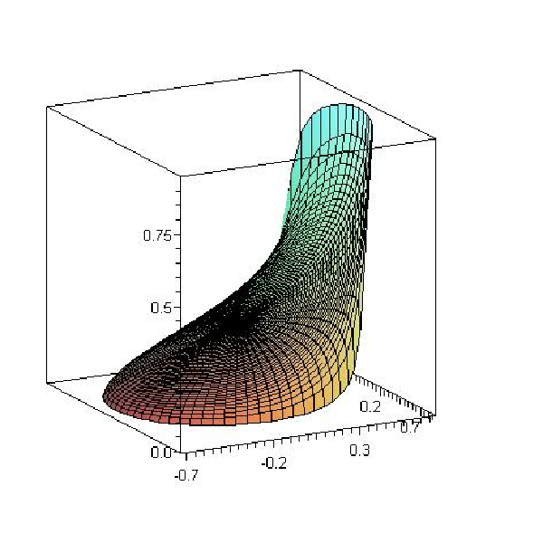
\mbox{\elevenss hom}(Q,(1,1,1))=(Z^{2}-\frac{1}{2}(U^{2}+V^{2}))(Y-Z)\,.

The zero set of this homogeneous polynomial is shown in Figure 10.

Let $T^{\prime}$ denote the flat torus ${\bf x}+{\mathbb{R}}^{d}/(2\pi{\mathbb{Z}})^{d}$ where ${\bf x}$ is any element of $B$ , the component of ${\mbox{\elevenss amoeba}}(Q)^{c}$ over which the series converges. Changing variables via ${\bf Z}=\exp({\bf z})=(e^{z_{1}},e^{z_{2}},e^{z_{3}})$ and $d{\bf z}=d{\bf Z}/{\bf Z}$ , then writing ${\bf z}={\bf x}+i{\bf y}$ and $f(\cdot)=F\circ\exp({\bf x}+i\cdot)$ , yields

a_{\bf r}=(2\pi)^{-d}e^{-{\bf r}\cdot{\bf x}}\int_{T^{\prime}}\exp(-i{\bf r}\cdot{\bf y})f({\bf y})\,d{\bf y}\,.

(3.4)

Up to this point the expression for $a_{\bf r}$ is exact. One can show that approximating $f$ by $\mbox{\elevenss hom}(f)$ and $T^{\prime}$ by ${\mathbb{R}}^{d}$ does not change the leading asymptotic term. This is a somewhat lengthy verification and it is here that the conical deformation of Corollary 3.10 is required. The upshot is that $a_{\bf r}=E({\bf r})$ where $E$ is the inverse Fourier transform of $\mbox{\elevenss hom}(f)$ . For quadratics, the inverse Fourier transform is the dual quadratic. For a product of a quadratic and a log-linear function, an explicit computation yields [BP11, Theorem 3.9]

C\arctan\left(\frac{\sqrt{A^{*}({\bf r},{\bf r})}\sqrt{-A^{*}(\ell,\ell)}}{A^{*}({\bf r},\ell)}\right)

where $A^{*}$ is the quadratic form dual to $\mbox{\elevenss hom}(f)$ and $\ell$ is the the log-linear factor viewed as an element of $({\mathbb{R}}^{d})^{*}$ in the logarithmic space. For example, when $F$ is the Aztec generating function one obtains the following result, a pictorial version of which is given in Figure 11.

Theorem 3.11 ([BP11, Theorem 3.7]).

The Northgoing placement probabilities $\{a_{rst}\}$ for the Aztec Diamond are asymptotically given by

a_{rst}\sim\frac{1}{\pi}\arctan\left(\frac{\sqrt{t^{2}-2r^{2}-2s^{2}}}{t-2s}\right)

when $(r,s,t)$ is in the cone $\{(r,s,t):t^{2}>2r^{2}+2s^{2}\}$ and $r+s+t$ is odd.

Remark.

The way the generating function is indexed, $a_{rst}=0$ when $r+s+t$ is even. Asymptotics in the corners of the diamond outside the inscribed circle are given by $a_{rst}\to 1$ in one corner and $a_{rst}\to 0$ in the other three, where convergence occurs at an exponential rate as $t\to\infty$ .

Part II: Stability

We now turn to the notion of stability. As we will see in Sections 4.3 and 5, the most useful properties of stability are closure properties: stability is preserved by a wealth of operations that are natural from an algebraic or probabilistic point of view. Stability is defined for general multivariate complex polynomials. Some of these properties or their proofs simplify when restricted to certain subclasses, such as polynomials whose coefficients are real or positive, or multi-affine polynomials, whose degrees in each variable never exceed 1. Even in these cases, however, some properties are proved only by going through the more general setting of complex coefficients.

4 Stability theory in one variable

As usual, the univariate theory is older and simpler. As with hyperbolicity, the origins of stability theory are in differential equations and control theory. After discussing this, we turn to combinatorial uses of the univariate theory. Stable generating polynomials produce coefficient sequences satisfying Newton’s inequalities, implying, among other things, log-concavity. We end the section on univariate stability with a discussion of stability preserving operations and the so-called Laguerre–Pólya class.

4.1 Stability over general regions

In this section we will begin by thinking more generally of polynomials that avoid roots in some region $\Omega$ . We will call these $\Omega$ -stable. Throughout the remainder of this paper we will let

{\cal H}:=\{z:\Im\{z\}>0\}\,.

denote the open upper half-plane. I will always use the term “stable” to mean ${\cal H}$ -stable, as in Definition 1.2, and will use “Hurwitz stable” or “ $\Omega$ -stable” for other notions of stability. Recalling G.-C. Rota’s philosophical observation, one might keep in mind that the Riemann Hypothesis is equivalent to $\Omega$ -stability where $\Omega=\{z:\Re\{z\}\neq 1/2\}$ . This may seem like a strained connection, but in fact some of the literature we review in Section 7 is explicitly motivated by the desire to understand the zeta function.

Statistical physicists have a different motive for understanding regions free of zeros. To explain this, we examine some graph theoretic models, paraphrasing the exposition in [Sok01]. Let $G=(V,E)$ be a finite graph and let $q$ be a positive integer. Define a polynomial in variables $\{x_{e}:e\in E\}$

Z(q,\{x_{e}:e\in E\}):=\sum_{\sigma}\prod_{e=\overline{vw}\in E}\left(1+x_{e}\delta_{\sigma(v),\sigma(w)}\right)

where $\sigma$ ranges over $q$ -colorings of the vertices, that is, all maps from $V$ to $\{1,\ldots,q\}$ . This is elementarily seen to be equivalent to the alternative definition

Z(q,\{x_{e}:e\in E\}):=\sum_{E^{\prime}\subseteq E}q^{k(E^{\prime})}\prod_{e\in E^{\prime}}x_{e}

where $k(E^{\prime})$ denotes the number of connected components in the subgraph $(V,E^{\prime})$ . The last formulation makes it obvious that $Z$ is a polynomial in $q$ as well as in $\{x_{e}\}$ . When $x_{e}=-1$ for all $e$ this specializes to the chromatic polynomial $\chi(q)$ ; more generally, taking $x_{e}=x$ for all $e$ gives the bivariate Tutte polynomial.

The polynomial $Z$ is also the partition function for the $q$ -state Potts model. Statistical physicists are interested in phase transitions where the behavior of the system depends non-analytically on its parameters. Being a polynomial, $Z$ is of course analytic in all its parameters. Typically though, one is interested in infinite-volume limits such as the free energy

f(q,x):=\lim_{n\to\infty}n^{-1}\log Z_{n}(q,x)

where $Z_{n}$ is taken on a graph $G_{n}$ in a family of graphs whose increasing limit is ${\mathbb{Z}}^{d}$ . The function $f$ may fail to be analytic at $(q,x)$ if the zeros of $Z_{n}(q,x)$ have a limit point at $(q,x)$ . Therefore, there is physical significance in keeping the zeros of the polynomial $Z_{n}$ out of specified regions. Such results are often known as Lee-Yang theorems, after [YL52, LY52] (see also [LS81]).

One such theorem was proved by D. Wagner in 2000. The reliability polynomial $R_{G}$ of the graph $G=(V,E)$ is the probability that the graph is connected when each edge is kept or deleted independently with probability $x$ , which is a polynomial in the parameter $x$ . Brown and Colbourn conjectured [BC92] that all zeros of $R_{G}(x)$ are in the closed disk $\{z:|z-1|\leq 1\}$ . In other words, $R_{G}$ is ${\cal D}^{c}$ -stable where ${\cal D}:=\{z:|z-1|\leq 1\}$ . This was proved for the class of series-parallel graphs in [Wag00, Theorem 0.2]. A simpler proof was found by Sokal [Sok01, Section 4.1, Remark 3], who actually proved the stronger multivariate stability result. On the other hand, Royle and Sokal [RS01] showed that the original univariate conjecture is false for general graphs; they also showed that multivariate ${\cal D}^{c}$ -stability of $R_{G}$ holds if and only if $G$ is series-parallel. Sokal [Sok11] has recently conjectured that $R_{G}$ is (univariate) ${\cal D}^{c}$ -stable for the complete graphs, $K_{n}$ .

Hurwitz stability

The association of zero-free regions with the term “stability” originated in ODE’s and control theory. Its use is attributed to Hurwitz. In fact, $\Omega$ -stability with $\Omega=\{z:\Re\{z\}\geq 0\}$ is sometimes called “Hurwitz stability”. In ODE’s, it is easy to see the physical significance of Hurwitz stability. Let $M$ be a matrix and consider the linear system ${\bf y}^{\prime}=M{\bf y}$ . Hurwitz stability is equivalent to all eigenvalues of $M$ having negative real parts, which is equivalent to all homogeneous solutions decaying, and hence good control over the system ${\bf y}^{\prime}-M{\bf y}={\bf v}(t)$ . One may also consider discrete-time analogues, such as the system ${\bf y}^{(n+1)}-Q{\bf y}^{(n)}={\bf v}^{(n)}$ where $Q$ would correspond to the exponential of $M$ in the previous system. Now decay of homogeneous solutions is equivalent to $\Omega$ -stability when $\Omega$ is the complement of the open unit disk; polynomials whose zeros are all in the open unit disk are said to be Schur-stable.

For a less trivial example we turn to control theory. Following [Hen91, Section 10.3], we consider systems which turn an input signal $f(t)$ into an output $u(t)$ . Many systems, and in particular those built from networks of impedances, are not only linear but also time homogeneous, that is, the map $f\mapsto u$ commutes with time translation. In terms of Laplace transforms, this means that the system acts multiplicatively, meaning that if ${\cal L}$ denotes the Laplace transform, then such systems obey the law

{\cal L}u=g\cdot{\cal L}f

(4.1)

for some function $g:[0,\infty)\to{\mathbb{R}}$ that is called the transfer function. For example an L-C-R circuit, with an input voltage function $f(t)$ between the inductor and the resistor producing an output $u(t)$ of current from the inductor to the capacitor, satisfies (4.1) with $g(s)=(R+Ls+C^{-1}/s)^{-1}$ . In impedance networks the transfer function is in fact always rational, $g(s)=p(s)/q(s)$ for some polynomials $p$ and $q$ . Generally, a system is said to be stable if bounded input produces bounded output.

To check whether the system with transfer function $g$ is stable, it suffices to test it on inputs of the form $f(t)=e^{i\omega t}$ , the Laplace transform of which is $({\cal L}f)(s)=1/(s-i\omega)$ . Let the poles of the rational function $g$ be $a_{1},\ldots,a_{r}$ . The ${\cal L}u=g\cdot{\cal L}f$ has poles $a_{1},\ldots,a_{r},i\omega$ . We may write ${\cal L}u$ in a partial fraction expansion resulting in $\sum_{j=0}^{r}p_{j}/(s-a_{j})$ for some polynomials $\{p_{j}\}$ ; here we have set $a_{0}:=i\omega$ . Inverting the Laplace transform gives a sum $\sum_{j=1}^{r}P_{j}(t)e^{a_{j}t}$ for some collection $\{P_{j}\}$ of polynomials. This is bounded if and only if each $a_{j}$ is either in the open left half-plane or is imaginary and a simple zero. But when $g$ has an imaginary zero $a_{j}$ , then setting $a_{0}=a_{j}$ (that is, taking the input to be $e^{ia_{j}t}$ ) produces a doubled root and an unbounded output. Hence, bounded inputs produce bounded outputs if and only if all poles of $g$ lie strictly in the left half-plane.

We conclude that stable behavior of the system corresponds to Hurwitz stability of the denominator of the transfer function $g$ . For example, in the L-C-R circuit above, the denominator of $g$ is a quadratic with positive coefficients. The real parts of the roots are always negative, whence such a system always behaves stably.

Differential equations of order $d$ may be transformed into first order systems in $d$ variables by the well known trick of representing the first $d-1$ derivatives as new variables. It is not surprising, therefore, that Hurwitz stability also arises in the stability analysis of order- $d$ linear differential equation with constant coefficients. Given $d$ initial conditions and an inhomogeneous term, we may write such an equation as

f^{(d)}+a_{d-1}f^{(d-1)}+\cdots+a_{0}f=H

(4.2)

with initial conditions $f^{(j)}(0)=b_{j}$ for $0\leq j\leq d-1$ . Assuming $H$ to grow at most exponentially, a Laplace transform exists near the origin. We may take the Laplace transfrom of both sides of (4.2). Using linearity and the rule ${\cal L}f^{\prime}(s)=s{\cal L}f(s)-f(0^{+})$ and denoting $g:={\cal L}f$ gives inductively

{\cal L}(f^{(d)})(s)=s^{d}g(s)-s^{d-1}f(0^{+})-s^{d-2}f^{\prime}(0^{+})-\cdots-f^{(d-1)}(0^{+})\,.

Plugging this and the boundary conditions into (4.2) yields the following equation for $g$ :

$\displaystyle s^{d}g(s)-s^{d-1}b_{0}-s^{d-2}b_{1}-\cdots-b_{d-1}$
$\displaystyle+\;a_{d-1}\left[s^{d-1}g(s)-s^{d-2}b_{0}-\cdots-b_{d-2}\right]$
$\displaystyle\vdots\hskip 36.135pt$
$\displaystyle+\;a_{1}\left[s^{1}g(s)-b_{0}\right]$
$\displaystyle+\;a_{0}g(s)$	$\displaystyle=$	$\displaystyle{\cal L}H(s)\,.$

Letting $p(s):=s^{d}+a_{d-1}s^{d-1}+\cdots+a_{0}$ denote the characteristic polynomial of the equation (4.2), and $p_{k}(s)$ denote the shifted polynomial $s^{k}+a_{d-1}s^{k-1}+\cdots+a_{d-k}$ , we may rewrite the equation for $g$ as

p\cdot g={\cal L}H+\sum_{j=0}^{d-1}b_{j}p_{d-1-j}

and hence

g(s)=\frac{{\cal L}H(s)+\sum_{j=0}^{d-1}b_{j}p_{d-1-j}(s)}{p(s)}\,.

(4.3)

Again, poles of $g$ with positive real part produce unbounded output, as do purely imaginary poles $i\omega$ when the driving term is taken to be $e^{i\omega t}$ , whose Laplace transform ${\cal L}H$ has a pole at $i\omega$ . Thus, again, Hurwitz stability is equivalent to bounded output on bounded input.

4.2 Real roots and Newton’s inequalities

I will now return, permanently, to upper half-plane stability, which will be called, simply, “stability”. In one variable, when the coefficients of $f$ are real, the zeros come in conjugate pairs. Stability, therefore, is equivalent to having only real zeros. When the coefficients are nonnegative, a strictly positive zero is impossible, whence stability is further equivalent to having all zeros on the negative half line.

Combinatorialists have long sought to exploit the properties of stable generating functions. The universal problem in combinatorial enumeration is to count a family of structures indexed by one or more positive integer parameters. In the case of one parameter, say $n$ , the sequence $\{a_{n}\}$ of counts and the corresponding generating function $f(z):=\sum_{n}a_{n}z^{n}$ are of fundamental interest. In the setting of probability generating functions, the coefficients $a_{n}$ are nonnegative and sum to one. In this case, if $f$ has only real roots, then the distribution which gives probability $a_{n}$ to the value $n$ is representable as the sum of independent random variables each taking the value 0 or 1 (Bernoulli random variables). There may or may not be a natural interpretation for these Bernoulli variables; see [HKPV09, Example 23] for an example in which there can be no natural interpretation.

Often it is intuitively plausible that the sequence $\{a_{n}\}$ is unimodal, meaning that for some $k$ , we have $a_{0}\leq\cdots\leq a_{k}\geq a_{k+1}\geq a_{k+2}\geq\cdots$ . The enumeration literature is littered with examples in which unimodality is conjectured (see for example the survey [Sta89] and the follow-up to this [Bre94]), but a proof is often elusive for the reason that there is no obvious theoretical framework within which to prove unimodality. There are, however some stronger properties for which natural avenues of proof exist.

Definition 4.1 (log-concavity).

A finite or infinite sequence $\{a_{k}\}$ of nonnegative numbers is said to have no internal zeros if the indices of the nonzero terms form an interval $[r,s]$ . The sequence is said to be log-concave if it has no internal zeros and if

a_{k-1}a_{k+1}\leq a_{k}^{2}

for $k\in[r+1,s-1]$ . The sequence $\{a_{r},\ldots,a_{r+k}\}$ with no internal zeros is said to be ultra log-concave if

\left(\frac{a_{j}}{\binom{k}{j}}\right)^{2}\geq\frac{a_{j+1}}{\binom{k}{j+1}}\;\frac{a_{j-1}}{\binom{k}{j-1}}\;.

It is immediate that ultra log-concavity implies log-concavity which implies unimodality. While ultra log-concavity appears to be the least natural of these properties, it was shown three centuries ago by Newton to follow from stability of the generating function.

Theorem 4.2 (Newton’s inequalities).

Suppose $f(z):=\sum_{k=0}^{n}a_{k}z^{k}$ is a real stable polynomial. Then for $1\leq k\leq n-1$ ,

\left(\frac{a_{k}}{\binom{n}{k}}\right)^{2}\geq\frac{a_{k+1}}{\binom{n}{k+1}}\;\frac{a_{k-1}}{\binom{n}{k-1}}\;.

(4.4)

If furthermore the coefficients $a_{k}$ are all nonnegative then the roots of $f$ are all nonpositive and the sequence is ultra log-concave.

Proof: By Rolle’s Theorem, if a univarite polynomial $f$ has only real zeros then so does its derivative. This observation will be useful many times below. We use it now to deduce that

Q(z):=\left(\frac{d}{dz}\right)^{k-1}f(z)

has only real zeros. Reversing a sequence of coefficients via $R(z):=z^{n-k+1}Q(1/z)$ also preserves the property of having all real roots. By Rolle’s Theorem again, $S(z):=(d/dz)^{n-k+1}R(z)$ has all real roots. But $S(z)$ is the trinomial

\frac{n!}{2}\left(\frac{a_{k-1}}{\binom{n}{k-1}}\;z^{2}+2\frac{a_{k}}{\binom{n}{k}}\;z+\frac{a_{k+1}}{\binom{n}{k+1}}\right)\,,

and the theorem follows from the discriminant test for quadratics. $\hfill\Box$

A curious result in a similar vein was proved by Gurvits [Gur08, Lemma 3.2]; the proof, which is a few lines of calculus, is omitted.

Proposition 4.3.

Let $f$ be a probability generating polynomial of degree $d$ and let $C:=\inf f(t)/t$ . If $f$ is stable then

a_{1}=f^{\prime}(0)\geq\left(\frac{d-1}{d}\right)^{d-1}\;C\,.

Equality holds if and only if $f=(1-q+qt)^{d}$ generates a binomial distribution. The value $[(d-1)/d]^{d-1}$ increases to $e^{-1}$ as $d\to\infty$ ; for infinite series, the bound $a_{1}\geq e^{-1}C$ holds with equality if and only if $f(t)=e^{\lambda(t-1)}$ is the generating function for a Poisson distribution. $\hfill\Box$

There are a number of techniques that can be used to establish stability (also known, in the univariate case, as the real root property). In some cases one has a sequence $\{f_{n}\}$ where $f_{n}$ has degree $n$ and the roots of $f_{n-1}$ interlace the roots of $f_{n}$ , meaning that each interval between roots of $f_{n}$ contains a root of $f_{n-1}$ . If this is true, then often it is possible to prove it by induction. The following example from [Sta89] illustrates this.

Example 4.4 (Hermite polynomials).

The Hermite polynomials are a sequence of polynomials defined by

H_{n}(z):=\sum_{k=0}^{\lfloor n/2\rfloor}\frac{(-1)^{k}n!(2z)^{n-2k}}{k!(n-2k)!}\,.

The are orthogonal with respect to the Gaussian measure $e^{-x^{2}}\,dx$ . They satisfy the recursion

H_{n}(z)=-e^{z^{2}}\frac{d}{dz}\left(e^{-z^{2}}H_{n-1}(z)\right)\,.

Assume for induction that $H_{n-1}(z)$ has $n-1$ real zeros. It is clear from this that $H_{n}$ has $n-2$ zeros interlacing the zeros of $H_{n-1}$ . To see that $H_{n}$ also has a zero less than all the zeros of $H_{n-1}$ , observe that $e^{-z^{2}}H_{n-1}$ tends to zero as $z\to-\infty$ , therefore $e^{-z^{2}}H_{n-1}$ has an extreme value to the left of its leftmost zero, which is a zero of $H_{n}$ . Similarly, $H_{n}$ has a zero greater than the greatest zero of $H_{n-1}$ , and the induction is established.

There is a more methodical way that often works to prove interlacing by induction. If $f$ and $g$ are real polynomials of respective degrees $n$ and $n-1$ having all real roots and the zeros of $g$ interlace the zeros of $f$ , it may be seen elementarily that $f+\lambda g$ has $n$ real zeros for any real $\lambda$ . A simple application of this idea is to the sequence $\{g_{n}\}$ defined by the three-term recurrence

g_{n+1}(x)=axg_{n}(x)+bg_{n-1}(x)\,,

which include the Chebyshev polynomials and Laguerre polynomials ( $a$ and $b$ depending on $n$ in the latter case). The same idea is the basis for a theorem independently proved by Heilmann and Lieb [HL72], by Gruber and Kunz [GK71] and, in part, by Nijenhuis [Nij76]. A matching on a finite weighted graph or multi-graph is a subset $M$ of the edge set such that any two edges in $M$ are disjoint (share no vertex). Fix a graph $G=(V,E)$ and let $\{W(e):e\in E\}$ be a set of nonnegative weights. Let $a_{j}$ denote the number of matchings with $j$ edges, counted by weight, where the weight of a matching is the product of the weights of the edges in the matching; by convention we take $a_{0}:-1$ . In the simplest case, $W(e)\equiv 1$ and $a_{j}$ simply counts matchings of size $j$ , size being the number of edges.

If we are allowed to set $W(e)=0$ for some edges, then the complete graph is universal. We therefore assume that $G=K_{n}$ for some $n$ .

Theorem 4.5 (matchings).

The number of weighted matchings of $K_{n}$ enumerated by size is ultra log-concave.

Proof: We show stability of a certain generating function, the most convenient being

Q_{n}(z):=\sum_{j=0}^{\lfloor n/2\rfloor}(-1)^{j}a_{j}z^{n-2j}\,.

(4.5)

This is monic, of degree $n$ , and is odd or even depending on $n$ . If we show $Q_{n}$ is stable and has $n$ distinct roots, then letting $Q_{n}(z)=R_{n}(z^{2})$ in the even case and $Q_{n}(z)=zR_{n}(z^{2})$ in the odd case, it follows that $R_{n}(-z)$ has $\lfloor n/2\rfloor$ negative real roots, hence is stable; it is also the generating function for matchings by size, hence the proof will be complete.

Taking limits at the end, we may assume without loss of generality that the weights $W(e)$ are all strictly positive. To see that $Q_{n}$ is stable, let $Q_{n}^{S}$ denote the generating function defined by (4.5) on the graph $K_{n}\setminus S$ . We use the recursion

Q_{n}(z)=zQ_{n}^{u}(z)-\sum_{v\neq u}W(u,v)Q_{n}^{u,v}(z)

(4.6)

which is obvious from the definition. The induction hypothesis is that $Q_{n}^{u}$ is stable with distinct roots, which are interlaced by the roots of $Q_{n}^{u,v}$ for any $v\neq u$ .

To verify the induction, we consider the sign of $Q_{n}$ at the $n-1$ zeros of $Q_{n}^{u}$ in decreasing order. By the interlacing property, the sign of each $Q_{n}^{u,v}$ alternates, starting out positive because $Q_{n}^{u,v}(+\infty)=+\infty$ . Therefore, $zQ_{n}^{u}-\sum_{v}W(u,v)Q_{n}^{u,v}$ alternates, starting out negative. This implies the existence of $n-2$ roots of $Q_{n}$ interlaced by the roots of $Q_{n}^{u}$ . But also there is one root of $Q_{n}$ to the right of every root of $Q_{n}^{u}$ because $Q_{n}$ is negative at the rightmost root of $Q_{n}^{u}$ and positive at $+\infty$ . Similarly there is one root of $Q_{n}$ to the left of every root of $Q_{n}^{u}$ . This completes the inductive proof. $\hfill\Box$

A second method by which one can establish univariate stability is via closure properties of the class of univariate stable polynomials. This topic will be expanded in the next section, but for now we mention a result from [Bre89], whose proof we will omit. Let $(x)_{i}$ denote the falling product $x(x-1)\cdots(x-i+1)$ and let $(x)^{i}$ denote the rising product $x(x+1)\cdots(x+i-1)$ .

Theorem 4.6 ([Bre89, Theorems 2.4.2–2.4.3]).

Let $f(x):=\sum_{k=0}^{n}a_{k}x^{k}$ be real stable with nonnegative coefficients. Then the polynomials $\sum_{k=0}^{n}a_{k}(x)_{k}$ and $\sum_{k=0}^{n}a_{k}(x)^{k}$ are real stable as well. $\hfill\Box$

In the following example, a function from the set $\{1,\ldots,n\}$ to itself is represented as a directed graph with an edge from $j$ to $f(j)$ for each $j$ .

Example 4.7 (functions enumerated by components).

Let $b(n,k)$ be the number of functions from the set $\{1,\ldots,n\}$ to itself whose directed graph has precisely $k$ components. It is elementary, cf. [GJ83, Example 3.3.28], that

b(n,k)=\sum_{i=1}^{n}\binom{n-1}{i-1}n^{n-i}c(i,k)

where $c(i,k)$ is a signless Stirling number of the first kind. Multiplying by $x^{k}$ and summing over $k$ gives

f_{n}(x):=\sum_{k=1}^{n}b(n,k)x^{k}=\sum_{i=1}^{n}\binom{n-1}{i-1}n^{n-i}(x)^{i}\,.

The corresponding sum replacing $(x)^{i}$ by $x^{i}$ has the short closed form

\sum_{i=1}^{n}\binom{n-1}{i-1}n^{n-i}x^{i}=x(x+n)^{n-1}\,.

Evidently this has only real zeros, so applying the conclusion of Theorem 4.6, we see that $f_{n}$ is stable as well.

A third method is an equivalent characterization for ultra log-concave that is due to Edrei [Edr53]. This relies on the notion of total positivity, a theme developed at length by Karlin [Kar68] and for which a number of combinatorial applications are given in [Bre95].

Definition 4.8 (Total positivity; Pólya frequency sequence).

$(i)$ An infinite matrix is said to be totally positive (TP) if all of its minors are nonnegative.

$(ii)$ A sequence $\{a_{n}\}$ is said to be a Pólya frequency sequence (PF-sequence) if the matrix $A_{nk}:=a_{n-k}$ is totally positive. Here we take $a_{i}:=0$ if $i<0$ or the sequence $\{a_{n}\}$ is finite and has length less than $i$ .

A proof of the following equivalence may be found in in [Kar68, Theorem 5.3].

Theorem 4.9 (Edrei’s equivalence theorem).

The nonnegative sequence $(a_{0},\ldots,a_{d})$ is a PF-sequence if and only if the generating polynomial $\sum_{k=0}^{d}a_{k}z^{k}$ is stable. $\hfill\Box$

Brenti [Bre94, Section 3] points out that only the $2\times 2$ minors are required for log-concavity, hence unimodality. Nevertheless, nonnegativity of all minors has a combinatorial interpretation which is given in [Bre95, Theorem 3.5]. This interpretation is somewhat abstract, but in special cases the interpretation can be more concrete.

Example 4.10 ( $r$ -derangements).

A permutation of $\{1,\ldots,n\}$ is said to be an $r$ -derangement if all its cycles have length at least $r$ . Thus a 1-derangement is any permutation, a 2-derangement is a classical derangement, and so forth. Let $b(n,r)$ count the number of $r$ -derangements of $\{1,\ldots,n\}$ . Brenti [Bre95, Corollary 5.9] shows that $f_{n}:=\sum_{r=1}^{n}b(n,r)z^{r}$ is stable. To do so, he shows that a related sequence $\{c_{r}(n)\}$ is a PF-sequence, hence stable, then applies Theorem 4.6 to recover the result with $b(n,r)$ in place of $c_{r}(n)$ .

We end this section with one more example of a stable generating polynomial, this one taken from [Sta89]. Recall from Example 2.4 that if $A$ is a real symmetric matrix and $B$ is real positive semi-definite then $f(z):={\rm Det\,}(A+zB)$ is a real stable polynomial.

Example 4.11 (spanning forests enumerated by component).

Let $G$ be a finite graph with possibly multiple edges and let

a_{k}(G):=\sum_{F}\gamma(F)

where the sum is over all spanning forests $F$ of $G$ such that $F$ has precisely $k$ components, where $\gamma(F)$ is the product of the cardinalities (numer of vertices) of the $k$ components. The factor of $\gamma$ changes the eumeration from forests to rooted forests. Following [Sta89, Proposition 4], let us see that the polynomial $f_{G}:=\sum_{k}a_{k}(G)z^{k}$ is stable. Let $A$ be the matrix whose rows and columns are indexed by the vertices of $G$ with entry $A_{ij}:=\deg(u)$ if $u=v$ and otherwise equal to $-N(i,j)$ where $N(i,j)$ is the number of edges between $i$ and $j$ . It is known that $f_{G}={\rm Det\,}(A+zI)$ . It follows that $f_{G}$ is stable. Therefore, the number of rooted forests enumerated by components is ultra log-concave, hence unimodal. Stanley attributes the identity $f_{G}={\rm Det\,}(A+zI)$ to Kelmans.

4.3 The Laguerre–Pólya class

Suppose we transform a polynomial $f(z)=\sum_{k=1}^{n}a_{k}z^{k}$ by multiplying each coefficient $a_{k}$ by a specified constant $\lambda_{k}$ . We may ask which sequences ${\boldsymbol{\lambda}}:=\{\lambda_{k}\}$ are multiplier sequences, meaning that the resulting operator $T_{\boldsymbol{\lambda}}$ preserves the class of real stable polynomials. A classical theorem due to Pólya and Schur [PS14] gives a complete and beautiful characterization of multiplier sequences.

Theorem 4.12 (Pólya-Schur 1914).

Let ${\boldsymbol{\lambda}}=\{\lambda_{n}:n\geq 0\}$ be a sequence of real numbers and let $T_{\boldsymbol{\lambda}}$ denote the linear operator defined by

T_{\boldsymbol{\lambda}}\left(\sum_{k=0}^{n}a_{k}z^{k}\right)=\sum_{k=0}^{n}\lambda_{k}a_{k}z^{k}\,.

Denote by $\Phi$ the formal power series

\Phi(z):=\sum_{k=0}^{\infty}\frac{\lambda_{k}}{k!}z^{k}\,.

Then the following are equivalent.

(i)

${\boldsymbol{\lambda}}$ is a multiplier sequence;
(ii)

$\Phi$ is an entire function and is the limit, uniformly on compact sets, of the polynomials with all zeros real and of the same sign;
(iii)

$\Phi$ is entire and either $\Phi(z)$ or $\Phi(-z)$ has a representation

$Cz^{n}e^{\alpha_{0}z}\prod_{k=1}^{\infty}(1+\alpha_{k}z)$

where $n$ is a nonnegative integer, $C$ is real, and $\alpha_{k}$ are real, nonnegative and summable.
(iv)

For all nonnegative integers $n$ , the polynomial $T_{\boldsymbol{\lambda}}[(1+z)^{n}]$ is real stable with all roots of the same sign.

We will not prove the general Pólya-Schur theorem here, proving only some special cases later as we need them. Some examples and remarks will clarify its meaning and possible uses. Condition $(iv)$ may be thought of as saying that the polynomials $(1+z)^{n}$ are universal test cases for stability preserving: a multiplier sequences preserving stability of these will preserve stability of all real stable polynomials.

Example 4.13 (dilation).

If $b$ is a nonnegative integer, setting $\lambda_{k}:=b^{k}$ produces the operator $T_{\boldsymbol{\lambda}}f(z)=f(bz)$ . Clearly this preserves stability. The representation in $(iii)$ is obvious because $\Phi(z)=e^{bz}$ .

Example 4.14 (factorials).

If $n\geq 1$ is an integer then the sequence $\lambda_{k}:=(n)_{k}:=n!/(n-k)!$ , defined to vanish when $k>n$ , produces the exponential generating function $\Phi(z)=(1+z)^{n}$ . By criterion $(iii)$ this is a multiplier sequence. Dividing by the constant $n!$ we see that $\lambda_{k}=1/(n-k)!$ for $k\leq n$ and zero for $k>n$ defines a multiplier sequence. For real polynomials of degree $n$ , stability of $f$ is equivalent to stability of the inversion $z^{n}f(1/z)$ , hence $\lambda_{k}=1/k!$ defines a multiplier sequence on polynomials of degree $n$ . This is true for every $n$ , whence $\{1/k!\}_{k=0}^{\infty}$ is a multiplier sequence. This result is due to Laguerre.

Example 4.15 (coefficientwise multiplication).

Applying the previous example to a polynomial $g(z)=\sum_{k=0}^{n}a_{k}z^{k}$ with negative real roots shows that $\sum_{k=0}^{n}(a_{k}/k!)z^{k}$ also has negative real roots. Setting $\lambda_{k}:=a_{k}$ for $k\leq n$ and zero for $k>n$ we see that its exponential generating function $\Phi(z)=\sum_{k=0}^{n}a_{k}z_{k}/k!$ is of the form in $(iii)$ with $\alpha_{0}=0$ . We conclude that $\{a_{k}\}$ is a multiplier sequence. In other words, if we multiply term by term the coefficient sequences of two real rooted polynomials, at least one of which has nonnegative coefficients, we get another real rooted coefficient sequence. Thus the real root property for polynomials with nonnegative coefficients is closed under Hadamard products.

Multiplier sequences are related to the so-called Laguerre–Pólya class. An entire function is said to be in the Laguerre–Pólya class, denoted ${\cal L}\hskip-3.0pt-\hskip-3.0pt{\cal P}$ , if it is the limit, uniformly on compact subsets of ${\mathbb{C}}$ , of polynomials with only real zeros; the terminology goes back at least to [Sch47]. It is said to belong to the subclass ${\cal L}\hskip-3.0pt-\hskip-3.0pt{\cal P}I$ if it is the limit of polynomials with only real zeros all of the same sign. Thus Theorem 4.12 asserts that generating functions of multiplier sequences are precisely the functions of class ${\cal L}\hskip-3.0pt-\hskip-3.0pt{\cal P}I$ .

A related notion to that of a multiplier sequence is the notion of a complex zero decreasing sequence (CZDS). Let $Z_{c}(f)$ denote the number of non-real zeros of $f$ . Say that a finite or infinite sequence $\{a_{k}\}$ is a CZDS if for any real polynomial $f(z)=\sum_{k=0}^{n}b_{k}z^{k}$ ,

Z_{c}\left(\sum_{k=0}^{n}a_{k}b_{k}z^{k}\right)\leq Z_{c}(f)\,.

(4.7)

In particular, in order for $\{a_{k}\}$ to be a CZDS, a value of zero on the right of (4.7) (no non-real zeros) implies no non-real zeros on the left, so any CZDS is a multiplier sequence. The converse, however, is not true.

To see that there is any nontrivial CZDS, we observe that the operator $z(d/dz)$ is represented by the sequence $a_{k}:=k$ and can never increase the number of non-real zeros. Although not every multiplier sequences is a CZDS, each multiplier sequence leads to a CZDS via the following result going back to Laguerre.

Proposition 4.16.

Let $\Phi\in{\cal L}\hskip-3.0pt-\hskip-3.0pt{\cal P}$ have zeros only in $(-\infty,0]$ . Then the sequence $\{\Phi(k):k\geq 0\}$ is a CZDS. $\hfill\Box$

Related to the notions of multiplier sequences and CZDS is the notion of a multiplier sequence for the property of being nonnegative on real inputs. Say that $\{c_{k}\}$ is a $\Lambda$ -sequence if multiplication of coefficients term by term preserves the property of being everywhere nonnegative:

\sum_{k=0}^{n}a_{k}x^{k}>0\mbox{ for all }x\in{\mathbb{R}}\Longrightarrow\sum_{k=0}^{n}c_{k}a_{k}x^{k}>0\mbox{ for all }x\in{\mathbb{R}}\,.

Note that negative values are allowed for the numbers $c_{k}$ . The following classical relationship is proved in [Wid41].

Proposition 4.17.

If $\{a_{k}\}$ is a CZDS then $\{a_{k}^{-1}\}$ is a $\Lambda$ -sequence. $\hfill\Box$

Connections abound between these notions: stability, multiplier sequences, the Laguerre–Pólya class, $\Lambda$ -sequences, etc., which we will not have time to survey here; the reader is referred to [CC95] for an introduction. $\Lambda$ -sequences, for example, are neatly characterized by a determinant condition and also by the so-called Hamburger moment problem: $\{c_{n}\}$ is a $\Lambda$ -sequence if and only if $c_{n}=\int_{-\infty}^{\infty}t^{n}\,d\mu(t)$ for some measure $\mu$ on ${\mathbb{R}}$ not supported on finitely many points. At the root of much of the present interest about these properties is their connection to the Riemann hypothesis. An account is given in [CV90, Cso03]. Finally, a small related literature on nonlinear transformations that preserve real stable polynomials may be of interest. It was conjectured independently by S. Fisk and R. Stanley that if the real polynomial $\sum_{k}a_{k}z^{k}$ has all real roots then so does the polynomial whose $z^{k}$ coefficient is $a_{k}^{2}-a_{k-1}a_{k+1}$ . Some progress was made by McNamara and Sagan in [MS10]; a proof of the conjecture and more was recently found by Brändén [Brä11].

5 Multivariate stability

Let ${\cal H}$ denote the open upper half-plane; thus stability is equivalent to having no zeros in the region ${\cal H}^{d}$ . We remark on some connections to other notions of stability. For homogeneous polynomials, the zero set is invariant under multiplication by $e^{i\theta}$ in each coordinate, therefore all notions of half-plane stability coincide. Any circular region (the interior or exterior of a circle) is transformed into ${\cal H}$ by a Möbius transformation, which allows the theory of $\Omega$ -stable functions to be mapped to the ordinary theory of stable functions via a bi-rational change of variables whenever $\Omega$ is the product of circular regions. This mapping acts nicely with respect to some aspects such as closure properties but not as nicely with respect to coefficient sequences. Thus, for example, it may shown that Schur-stability, where $\Omega={\cal D}^{d}$ and ${\cal D}$ is the open unit disk, has an unexpected closure property: if $f$ and $g$ are multi-affine Schur-stable polynomials then the Hadamard product $f\bullet g$ is Schur-stable as well; here the Hadamard product of $\sum_{S}a(S){\bf z}^{S}$ and $\sum_{S}b(S){\bf z}^{S}$ is defined to be $\sum_{S}a(S)b(S){\bf z}^{S}$ . Our principal interest is in ${\cal H}$ -stable polynomials and their coefficients. We will not henceforth consider notions of stability other than upper half-plane stability.

A number of the closure properties of the class of stable polynomials extend immediately from the univariate to the multivariate setting or are otherwise elementary. In particular, if $f\in{\mathbb{C}}[z_{1},\ldots,z_{d}]$ is stable then so are the polynomials obtained by the following operations:

(a)

dilation: replacing $f$ by $f(b_{1}z_{1},\ldots,b_{d}z_{d})$ , where $\{b_{j}\}$ are nonnegative constants;
(b)

permuting the names of the variables;
(c)

specialization: setting $z_{j}$ equal to a constant in ${\cal H}$ ;
(d)

diagonalization: setting $z_{j}$ equal to $z_{i}$ ;
(e)

inversion: replacing $f$ by $f(-1/z_{1},z_{2},\ldots,z_{d})$ ;
(f)

differentiation: replacing $f$ by $\partial f/\partial z_{j}$ ;
(g)

limits: $f_{n}\to f$ uniformly on compact sets and $f_{n}$ stable implies $f$ is stable;

see for example [Wag11, Lemma 2.4]; here, and after, in results such as the this one, we will take “stable” to include the zero polynomial in order not to have to make exceptions.

We also recall that Proposition 1.3 equates stability of a real homogeneous polynomial to hyperbolicity in all directions in the positive orthant. Although the definition of hyperbolicity is more complicated for non-homogeneous polynomials, the corresponding fact characterization of real stable polynomials is not.

Proposition 5.1.

A (non identically zero) real $d$ -variable polynomial $f$ is stable if and only if for all ${\bf v}\in{\mathbb{R}}^{d}$ and ${\bf u}\in{\mathbb{R}}^{d}_{+}$ , the polynomial $t\mapsto f({\bf v}+t{\bf u})$ has only real zeros.

Proof: If $f$ has a zero $(z_{1},\ldots,z_{d})$ in ${\cal H}^{d}$ , then writing $z_{j}=v_{j}+iu_{j}$ , we see that ${\bf u}\in{\mathbb{R}}^{d}_{+}$ and $i$ is a zero of $f({\bf v}+t{\bf u})$ . Conversely, if ${\bf u}\in{\mathbb{R}}^{d}_{+}$ and ${\bf v}\in{\mathbb{R}}^{d}$ such that $f({\bf v}+t{\bf u})$ has a root with nonvanishing imaginary part, we may conjugate if necessary to find a root $t=a+bi$ with $b>0$ ; then ${\bf v}+t{\bf u}$ is a zero of $f$ in ${\cal H}^{d}$ . $\hfill\Box$

There is one geometric feature of functions of two or more complex variables, absent from the univariate theory, that is worth noting because it strengthens closure property (c). Let $f$ be any function in $d$ variables, vanishing at ${\bf b}=(b_{1},\ldots,b_{d})$ and analytic in a neighborhood of ${\bf b}$ . Suppose that $f(\cdot,b_{2},\ldots,b_{d})$ is not the zero function. Then there is a continuous multi-valued function $\phi$ on a neighborhood $U$ of $(b_{2},\ldots,b_{d})$ in ${\mathbb{C}}^{d-1}$ such that $\phi({\bf z})\to b_{1}$ as ${\bf z}\to(b_{2},\ldots,b_{d})$ and such that $f(\phi({\bf z}),{\bf z})=0$ . This perturbation property follows from the fact that at least one multivariate Puiseux series solution exists for $z_{1}$ as a function of $z_{2},\ldots,z_{d}$ which converges to $b_{1}$ . This leads to the following lemma.

Lemma 5.2.

Let $B_{j},1\leq j\leq d$ be open subsets of ${\mathbb{C}}$ . Suppose a polynomial $f$ is nonvanishing on $\prod_{j=1}^{d}B_{j}$ . Then $f$ is nonvanishing on $\prod_{j=1}^{d}\overline{B_{j}}$ except possibly in two cases: $f$ can vanish on the product of boundaries $\prod_{j=1}^{d}\partial B_{j}$ , and $f$ can vanish at a point $(b_{1},\ldots,b_{d})$ with coordinates $\{b_{j}:j\in S\}$ in the interior of $B_{j}$ for some set $S\subseteq\{1,\ldots,d\}$ provided that $f$ vanishes identically for all values of those coordinates, that is, $f(b_{1}^{\prime},\ldots,b_{d}^{\prime})=0$ whenever $b_{j}^{\prime}=b_{j}$ for all $j\notin S$ .

In particular, taking $B_{j}={\cal H}$ for all $j$ , we see that stability implies no zeros in $\overline{{\cal H}}^{d}$ except for real zeros or degenerate cases.

A further consequence of this lemma is that (c) can be strengthened to include setting $z_{j}$ equal to a real constant.

Proof: Let $f$ vanish at ${\bf b}=(b_{1},\ldots,b_{d})$ where $b_{j}\in\partial B_{j}$ for $j\leq r$ and $b_{j}\in B_{j}$ for $j>r$ . We need to show that the hypotheses are contradicted if $k>r$ is a coordinate such that $f$ does not vanish identically when the remaining coordinates are fixed. This follows if we perturb each coordinates $b_{j},j\neq k$ so as to lie in the open region $B_{j}$ , by sufficiently small amounts so that the perturbation solution for $z_{k}$ lies in $B_{k}$ . $\hfill\Box$

The above facts are generally quite elementary. Before we get to the fun stuff, there is some serious overhead in deriving further closure properties. One route to developing properties of multivariate stable functions is via the notion of proper position. This is in some sense a multivariate version of interlacing of roots. The development here specifically avoids this because I do not find it intuitive and because we can do everything we need without it. For a development incorporating the notion of proper position, see [Wag11].

5.1 Equivalences

Recall from Proposition 1.3 the relation between stability and hyperbolicity: a real homogeneous polynomial is stable if and only if it has a cone of hyperbolicity containing the (strictly) positive orthant. A number of equivalent formulations of stability will prove useful. If $f\in{\mathbb{C}}[z_{1},\ldots,z_{d}]$ is any polynomial, let $m$ denote the maximum total degree of any monomial in $f$ and define the homogenization $f_{H}$ of $f$ to be the unique degree- $m$ homogeneous polynomial in the variables $z_{1},\ldots,z_{d+1}$ such that $f_{H}(z_{1},\ldots,z_{d},1)=f(z_{1},\ldots,z_{d})$ . We may write explicitly $f_{H}(z_{1},\ldots,z_{d+1})=z_{d+1}^{m}\,f(z_{1}/z_{d+1},\ldots,z_{d}/z_{d+1})$ . The following proposition is proved in [BBL09, Section 4].

Proposition 5.3 (homogenization).

The real polynomial $f\in{\mathbb{R}}[z_{1},\ldots,z_{d}]$ is stable if and only if the homogeneous polynomial $f_{H}$ is hyperbolic in all directions ${\bf v}$ such that $v_{j}>0$ for $1\leq j\leq d$ and $v_{d+1}=0$ .

If $f$ also has nonnegative coefficients then the four properties are all equivalent:

(i)

$f$ is stable;
(ii)

$f_{H}$ is stable;
(iii)

$f_{H}$ is hyperbolic with respect to some vector in the nonnegative orthant;
(iv)

$f_{H}$ is hyperbolic with respect to every vector in the positive orthant.

Proof: For one direction, assume $f_{H}$ to be hyperbolic in every direction ${\bf y}$ with $y_{j}$ positive when $j\leq d$ and $y_{d+1}=0$ . For any ${\bf x}\in{\mathbb{R}}^{d}$ and ${\bf y}\in{\mathbb{R}}_{+}^{d}$ , the polynomial

t\mapsto f({\bf x}+t{\bf y})=f_{H}(({\bf x},1)+t({\bf y},0))

is not identically zero because $\lim_{t\to\infty}t^{-m}f({\bf x}+t{\bf y})$ is equal to $f_{H}({\bf y},0)\neq 0$ . It has only real zeros, by hyperbolicity of $f_{H}$ in direction $({\bf y},0)$ , hence $i$ is not a root, hence $f({\bf x}+i{\bf y})\neq 0$ ; but ${\bf x}\in{\mathbb{R}}^{d}$ and ${\bf y}\in{\mathbb{R}}_{+}^{d}$ are arbitrary, so this is stability of $f$ .

For the other direction, suppose $f_{H}$ fails to be hyperbolic in a direction ${\bf v}$ for which $v_{j}>0,1\leq j\leq d$ , and $v_{d+1}=0$ . Then $f_{H}({\bf x}+t{\bf v})$ has a non-real zero $t=u$ for some ${\bf x}\in{\mathbb{R}}^{d+1}$ . The complex conjugate of $u$ is also a zero so we may assume without loss of generality that the imaginary part of $u$ is positive. The vector ${\bf y}:={\bf x}+u{\bf v}$ lies in ${\cal H}^{d}\times{\mathbb{R}}$ . There are three cases. First, if $y_{d+1}>0$ then dividing though by this gives a zero of $f$ in ${\cal H}^{d}$ , implying $f$ is not stable. Second, if $y_{d+1}<0$ , dividing yields a zero in $-{\cal H}^{d}$ and conjugating, we see again that $f$ is not stable. Finally, if $y_{d+1}=0$ , we may use perturbation to reduce to the case where $y_{d+1}\neq 0$ .

For the equivalence of the four properties in the case of nonnegative coefficients, recall that the cone of hyperbolicity of $f_{H}$ containing some vector ${\bf v}$ is the connected component in ${\mathbb{R}}^{d+1}$ that contains ${\bf v}$ of the set where $f_{H}$ is nonzero. By nonnegativity of the coefficients, if this cone contains any vector in the closed nonnegative orthant then it contains all vectors in the positive orthant. This establishes the equivalence of (iii) and (iv). Equivalence between (iii) and (ii) is Proposition 1.3. Finally, we note that (ii) implies (i) by setting $z_{d+1}=1$ (as is allowed by the last consequence of Lemma 5.2), while (i) implies (iii) by the first part of this proposition. $\hfill\Box$

Remark.

The perturbation argument also proves that stability of $f$ implies stability of $\mbox{\elevenss hom}(f)$ , where $\mbox{\elevenss hom}(f)(z_{1},\ldots,z_{d}):=f_{H}(z_{1},\ldots,z_{d},0)$ is the leading homogeneous part of $f$ ; see, e.g., [COSW04, Proposition 2.2].

The special case of multi-affine polynomials

Suppose $f$ is multi-affine, that is, no variable appears in any monomial with power two or higher. The following equivalence is taken by some to be the definition of stability in the multi-affine case. Its significance will become evident in the next section.

Theorem 5.4 ([Brä07, Theorem 5.6]).

Let $f$ be real and multi-affine. Then $f$ is stable if and only if the inequality

\frac{\partial f}{\partial x_{i}}({\bf x})\frac{\partial f}{\partial x_{j}}({\bf x})\geq f({\bf x})\frac{\partial^{2}f}{\partial x_{i}\partial x_{j}}({\bf x})

(5.1)

holds for all real ${\bf x}$ and distinct $i,j\leq n$ .

The proof given here is considerably simpler than the published proof, which is a “proper position” argument. It comes from the same source (P. Brändén, personal communication) and begins with the following lemma.

Lemma 5.5.

Let $Q,R\in{\mathbb{C}}[z_{1},\ldots,z_{n}]$ and define $P=Q+z_{n+1}R\in{\mathbb{C}}[z_{1},\ldots,z_{n+1}]$ . Let $\Omega\subseteq{\mathbb{C}}^{n}$ be any connected set and let $D_{1},D_{2}$ be closed subsets of ${\mathbb{C}}$ with disjoint interiors, such that $D_{1}\cup D_{2}={\mathbb{C}}$ and $J:=D_{1}\cap D_{2}$ a simple curve separating $D_{1}$ and $D_{2}$ .

If $P$ has no roots in $\Omega\times J$ and $R$ has no roots in $\Omega$ then $P$ either has no roots in $\Omega\times D_{1}$ or has no roots in $\Omega\times D_{2}$ .

Proof: $P$ having no roots in $\Omega\times J$ is equivalent to $-Q({\bf z})/R({\bf z})\notin J$ for all ${\bf z}\in\Omega$ . Hence $-Q/R$ maps $\Omega$ either to the interior of $D_{1}$ or the interior of $D_{2}$ , hence to $D_{2}^{c}$ or $D_{1}^{c}$ , and the result follows. $\hfill\Box$

Proof of theorem: For the forward implication, suppose $f$ is stable. Let $e_{i}$ denote the $i^{th}$ standard basis vector and define $G(s,t):=f({\bf x}+te_{i}+se_{j})$ . For any ${\bf x}\in{\mathbb{R}}^{d}$ , the function $G$ is stable in the variables $(s,t)$ . To see this, note that this is equivalent to $f$ having no zeros in $\overline{{\cal H}}^{d}$ with coordinates $i$ and $j$ in ${\cal H}$ ; this is ruled out by Lemma 5.2. By multi-affinity, we may express $G$ as $a+bs+ct+dst$ where $a,b,c,d$ are given by partial derivatives:

G(s,t)=f({\bf x})+\frac{\partial f}{\partial z_{i}}({\bf x})s+\frac{\partial f}{\partial z_{j}}({\bf x})t+\frac{\partial^{2}f}{\partial z_{i}\partial z_{j}}({\bf x})st\,.

For bivariate multi-affine polynomials $a+bs+ct+dst$ , stability is equivalent to $ad\leq bc$ , and the forward direction follows.

For the reverse direction, use induction on $n$ . When $n=1$ the result is true because all nonzero real polynomials $a+bx$ are stable. Assume the reverse result for $n$ and suppose $P=Q+z_{n+1}R$ satisfies (5.1). If $Q$ or $R$ is identically zero then we are done by induction, so assume not. For any real $x$ , it is clear that $P(z_{1},\ldots,z_{n},x)$ satisfies (5.1), hence, by induction, the polynomials $Q,R$ and $Q+xR$ are all stable or identically zero. If $Q+\alpha R\equiv 0$ for some real $\alpha$ then $P=(z_{n+1}-\alpha)R$ which is stable. We may assume, therefore, that there is no $\alpha$ for which $Q+\alpha R$ is identically zero. It follows that $P$ has no zeros in $H^{n}\times{\mathbb{R}}$ where $H$ is the open upper half-plane. By Lemma 5.5 this implies that either $P$ or $P(z_{1},\ldots,z_{n},-z_{n+1})$ is stable. In the latter case, by the forward direction, equation (5.1) holds with the signs reversed for $j=n+1$ and $i\leq n$ , and hence with equality for such $i$ and $j$ . This works out to $(\partial R/\partial x_{i})Q=(\partial Q/\partial x_{i})R$ for all $i\leq n$ , that is, $Q$ and $R$ are multiples of each other, which again implies that $P$ is stable. $\hfill\Box$

5.2 Operations preserving stability

In a brilliant series of papers [BB09a, BB09b, BB10], Borcea and Brändén finished off the problem of extending the Pólya-Schur Theorem to multivariate stability preserving maps. This work not only generalizes from one variable to several, but also from multiplier sequences to arbitrary ${\mathbb{C}}$ -linear maps. I will present here two of their results, one for multiplier sequences and one giving universal test functions for general linear maps, proving only those parts that will be of use later.

As before, if ${\boldsymbol{\lambda}}=\{\lambda_{\bf r}:{\bf r}\in{\mathbb{Z}}_{+}^{d}\}$ is an array of real numbers, we denote by $T_{\boldsymbol{\lambda}}$ the operator for which

T_{\boldsymbol{\lambda}}\left(\sum_{\bf r}a_{\bf r}{\bf z}^{\bf r}\right)=\sum_{\bf r}\lambda_{\bf r}a_{\bf r}{\bf z}^{\bf r}\,.

Also generalizing from before, we say that ${\boldsymbol{\lambda}}$ is a multivariate multiplier sequence if $T_{\boldsymbol{\lambda}}$ preserves the class of real stable polynomials. The following theorem is proved in [BB10, Theorem 1.8].

Theorem 5.6 (multivariate multiplier sequences).

The array ${\boldsymbol{\lambda}}$ is a $d$ -variate multiplier sequence if and only if there are $d$ univariate multiplier sequences ${\boldsymbol{\lambda}}^{(1)},\ldots,{\boldsymbol{\lambda}}^{(d)}$ such that

\lambda_{\bf r}=\lambda^{(1)}_{r_{1}}\cdots\lambda^{(d)}_{r_{d}}

and satisfying a further sign condition: either every $\lambda_{\bf r}$ is nonnegative, or every $\lambda_{\bf r}$ is nonpositive, or the same holds for $(-1)^{|{\bf r}|}{\boldsymbol{\lambda}}$ .

Proof in one direction: The easy direction, and all we will need below, is to see that the product of univariate nonnegative multiplier sequences is a multiplier sequence (also that nonnegative multiplier sequences preserve complex stability, not just real stability). Let $\lambda_{\bf r}=\prod_{j=1}^{d}\lambda^{(j)}_{r_{j}}$ where each sequence ${\boldsymbol{\lambda}}^{(j)}$ is a univariate multiplier sequence. First assume that $\lambda^{(j)}$ is identically 1 for $j\geq 2$ . Let $f$ be a real stable polynomial of $d$ variables. Fixing $z_{2},\ldots,z_{d}$ in the upper half-plane, the polynomial $f_{1}:=f(\cdot,z_{2},\ldots,z_{d})$ is univariate stable, and by the stability preserving assumption on ${\boldsymbol{\lambda}}^{(i)}$ , we see that $T_{{\boldsymbol{\lambda}}_{1}}(f_{1})$ is univariate stable. This polynomial having no zeros in the upper half-plane is equivalent to $T_{\boldsymbol{\lambda}}f$ having no zeros with $z_{1}$ in the upper half-plane and the specified values of $z_{2},\ldots,z_{d}$ . Because these values were arbitrary values in the upper half-plane, this finishes the proof in this special case. For the general case, write $T_{\boldsymbol{\lambda}}$ as the composition of operators of this form in each coordinate. $\hfill\Box$

One consequence of this is that the multi-affine part of a stable polynomial is stable.

Corollary 5.7.

Let $f$ be a stable polynomial in $d$ variables and let $f_{\rm ma}$ denote the multi-affine part of $f$ , that is, the sum of the square-free monomials in $f$ . Then $f_{\rm ma}$ is stable.

Proof: The sequence $a_{0}=1,a_{1}=1,a_{n}=0$ for $n\geq 2$ is a multiplier sequence. By Theorem 5.6, the multivariate sequence defined by ${\boldsymbol{\lambda}}_{\bf r}=1$ if ${\bf r}_{j}=0$ or 1 for all $j\leq d$ and ${\boldsymbol{\lambda}}_{\bf r}=0$ otherwise is a multiplier sequence. This multiplier sequence extracts the multi-affine part. $\hfill\Box$

A complete characterization of linear operators preserving stability of complex polynomials was proved in [BB09a, Theorem 2.3]. We will discuss here only the version of this result concerning operators preserving stability of multi-affine functions. We need to define what Borcea and Brändén call the algebraic symbol $G_{T}$ of a linear operator $T$ . Their definition requires a degree bound on each variable. We consider here only the multi-affine case; if you compare to the original text, you should set the degree bound vector $\kappa$ to $(1,\ldots,1)$ . Let ${\mathbb{C}}_{\rm ma}[z_{1},\ldots,z_{d}]$ denote the space of complex multiaffine polynomials in $d$ variables. For a linear operator $T:{\mathbb{C}}_{\rm ma}[z_{1},\ldots,z_{d}]\to{\mathbb{C}}[z_{1},\ldots,z_{d}]$ define its algebraic symbol to be the element $G_{T}\in{\mathbb{C}}[z_{1},\ldots,z_{d},w_{1},\ldots,w_{d}]$ satisfying

G_{T}(z_{1},\ldots,z_{d},w_{1},\ldots,w_{d})=\sum_{S\subseteq\{1,\ldots,d\}}\prod_{j\notin S}w_{j}T\left(\prod_{j\in S}z_{j}\right)\,.

(5.2)

In other words, $G$ applies $T$ to $\prod_{j=1}^{d}(z_{j}+w_{j})$ by treating $\{w_{j}\}$ as constants and applying $T$ to the resulting monomials in $\{z_{j}\}$ .

Theorem 5.8 ([BB09a, Lemma 3.2]).

Let $T:{\mathbb{C}}_{\rm ma}[z_{1},\ldots,z_{d}]\to C[z_{1},\ldots,z_{d}]$ be any ${\mathbb{C}}$ -linear operator. Then $T$ preserves stability if and only one of the two following conditions hold:

(a)

There is a stable polynomial $P$ and a linear functional $\alpha:{\mathbb{C}}_{\rm ma}[z_{1},\ldots,z_{d}]\to{\mathbb{C}}$ such that $T(f)=\alpha(f)P$ ;
(b)

The polynomial $G_{T}(z_{1},\ldots,z_{d},w_{1},\ldots,w_{d})$ is stable as a complex polynomial in $2d$ variables.

Remark.

This is a very powerful theorem and it is worth asking what part of it one needs to understand in order to understand the Borcea–Brändén–Liggett theory of negatively dependent random variables surveyed in Section 6. The answer is that we only use one direction (sufficiency) and this is only to prove Proposition 6.17, which could be proved elementarily as it concerns only bivariate functions. Nevertheless, because this would be messy and unenlightening, we will prove the sufficiency direction of Theorem 5.8 here, which we will then use to prove Proposition 6.17. The proof relies on a lemma proved thirty years ago by Lieb and Sokal [LS81], which we will not prove here (the proof is half a page in [Wag11]).

Lemma 5.9 ([LS81, Lemma 2.3]).

Let $P({\bf z})+wQ({\bf z})$ be stable in ${\mathbb{C}}[z_{1},\ldots,z_{d},w]$ . If the degree of the variable $z_{j}$ is at most 1 then the polynomial

P({\bf z})-\frac{\partial Q({\bf z})}{\partial z_{j}}

is either identically zero or is stable. $\hfill\Box$

Proof of sufficiency: If $T$ satisfies $(a)$ the result is immediate, so assume $T$ satisfies (b). Because $w\mapsto-w^{-1}$ preserves ${\cal H}$ , we see that $G_{T}({\bf z},{\bf w})$ is stable if and only if $w_{1}\cdots w_{d}G_{T}({\bf z},-{\bf w}^{-1})$ is stable; here $-{\bf w}^{-1}$ denotes $(-w_{1}^{-1},\ldots,-w_{d}^{-1})$ . From this, we see that if $f\in{\mathbb{C}}[v_{1},\ldots,v_{d}]$ is stable and multi-affine, then

(w_{1}\cdots w_{d})\cdot G_{T}({\bf z},-{\bf w}^{-1})\cdot f({\bf v})=\sum_{S\subseteq\{1,\ldots,n\}}T[{\bf z}^{S}](-{\bf w})^{S}f({\bf v})

(5.3)

is stable in ${\mathbb{C}}[{\bf z},{\bf w},{\bf v}]$ . We now apply the Lieb-Sokal lemma $d$ times: the $j^{th}$ time we take $w=w_{j}$ and $z_{j}=v_{j}$ . Each time, the Lieb Sokal lemma replaces $w_{j}$ in (5.3) by $-(\partial/\partial v_{j})$ . The final result is that

\sum_{S\subseteq\{1,\ldots,n\}}T[{\bf z}^{S}]f^{(S)}({\bf v})

(5.4)

is stable in ${\mathbb{C}}[{\bf z},{\bf v}]$ . Specializing each $v_{j}$ to zero preserves stability. But this specialization yields $\sum_{S}f^{(S)}(0)T[z^{S}]$ , which is another name for $Tf({\bf z})$ . Thus stability of $f$ implies stability of $Tf$ , proving the theorem. $\hfill\Box$

5.3 More closure properties

The multivariate Pólya-Schur theorems of Borcea and Brändén are powerful but there are yet more closure properties that are useful in probabilistic settings because they have specific probabilistic meanings. We state these now but defer the proofs to the next section.

Let $n_{j},1\leq j\leq d$ be the maximum degree of the variable $z_{j}$ in a given polynomial $f\in{\mathbb{C}}[z_{1},\ldots,z_{d}]$ . One natural way to create a multi-affine polynomials out of $f$ is to replace each occurrence of each power $z_{j}^{r}$ by $\binom{n_{j}}{r}^{-1}e_{r}(z_{j,1},\ldots,z_{j,n_{j}})$ , where $e_{r}$ is the $r^{th}$ elementary symmetric function. Here $\{z_{j,s}:1\leq j\leq d,1\leq s\leq n_{j}\}$ are a collection of clone variables. Formally, define the polarization $f_{p}$ of $f$ to be the unique polynomial symmetric separately in each set of clone variables $z_{j,1},\ldots,z_{j,n_{j}}$ such that substituting the value $z_{j}$ for all the clones $z_{j,s}$ yields the original function $f$ . In Section 6.4 we will show that stability is closed under polarization.

One final useful closure result is the following. The proof will be given after a probabilistic interpretation is given in Section 6.4.3.

Theorem 5.10 (partial symmetrization).

Let $f$ be a $d$ -variate complex poynomial. Fix $1\leq i<j\leq d$ and define $\tau f$ to be $f$ with the roles of $z_{i}$ and $z_{j}$ swapped:

\tau f(z_{1},\ldots,z_{d})=f(z_{1},\ldots z_{i-1},z_{j},z_{i+1},\ldots,z_{j-1},z_{i},z_{j+1},\ldots,z_{d})\,.

Fix $\theta\in[0,1]$ and define $f_{\theta;i,j}:=(1-\theta)f+\theta\tau(f)$ . If $f$ is stable, so is $f_{\theta;i,j}$ .

6 Negative dependence

6.1 A brief history of negative dependence

When random variables in a collection influence each other in a consistent direction, this can be very useful for obtaining one-sided bounds on moments and probabilities of natural events. For example, when all pairwise correlations are negative, the variance of the sum is bounded above by the sum of the variances. For this reason, the literature is sprinkled with definitions of various properties of positive and negative dependence, that hold in examples of interest and which imply useful consequences. Some of these apply to random variables taking values in ${\mathbb{R}},{\mathbb{R}}^{+},{\mathbb{Z}}$ or ${\mathbb{Z}}^{+}$ . To keep matters simple and coherent, we will discuss only the case where the variables are binary valued, that is, take values in the set $\{0,1\}$ . The joint law of $d$ binary variables is a probability measure on ${\cal B}_{d}:=\{0,1\}^{d}$ .

The simplest and one of the weakest conditions is pairwise positive (respectively negative) correlation: ${\mathbb{E}}X_{i}X_{j}\geq({\mathbb{E}}X_{i})({\mathbb{E}}X_{j})$ (respectively $\leq$ ), which may also be written as ${\mathbb{P}}(X_{i}=X_{j}=1)\geq{\mathbb{P}}(X_{i}=1){\mathbb{P}}(X_{j}=1)$ (respectively $\leq$ ). As we have just seen, this condition is strong enough to imply one-sided bounds on the variance of $\sum_{j}X_{j}$ . It is not strong enough to give bounds on the moments. For this, one requires at least positive or negative cylinder dependence. Positive cylinder dependence is said to hold if

{\mathbb{E}}\prod_{j\in S}X_{j}\geq\prod_{j\in S}{\mathbb{E}}X_{j}

(6.1)

for all subsets $S\subseteq\{1,\ldots,n\}$ . Negative cylinder dependence is the reverse inequality. Sometimes this is strengthened to require as well that

{\mathbb{E}}\prod_{j\in S}(1-X_{j})\geq\prod_{j\in S}(1-{\mathbb{E}}X_{j})\,.

(6.2)

The equation (6.1) immediately implies that the moments of $Z:=\sum_{j}X_{j}$ are at least what they would be for independent Bernoullis with the same marginals, while negative cylinder dependence implies the moments are at most what they would be in the independent case. Expanding the moment generating function $\phi(\lambda):={\mathbb{E}}e^{\lambda Z}$ in powers of $Z$ , and then into monomials in the variables $X_{j}$ shows that positive (respectively negative) cylinder dependence implies that for $\lambda\geq 0$ , the moment generating function $\phi(\lambda)$ is at least (respectively at most) what it would be for independent Bernoullis of the same marginal; including the inequality for complementary cylinders (6.2) extends the inequality for moment generating functions to $\lambda<0$ . The bounds on moment generating functions transfer to concentration inequalities (see, e.g., [PS97, Theorem3.4]).

A yet stronger property is association. Say that the collection of random variables $\{X_{1},\ldots,X_{d}\}$ is positively associated if

{\mathbb{E}}f(X_{1},\ldots,X_{d})g(X_{1},\ldots,X_{d})\geq{\mathbb{E}}f(X_{1},\ldots,X_{d})({\mathbb{E}}g(X_{1},\ldots,X_{d})

whenever $f,g:{\cal B}_{d}\to{\mathbb{R}}$ are nondecreasing functions (with respect to the coordinatewise partial order on ${\cal B}_{d}$ ). Negative association cannot be defined by simply reversing the inequality because any function $f$ is always nonnegatively correlated with itself. Therefore, we amend the definition to say that $\{X_{1},\ldots,X_{d}\}$ are negatively associated if ${\mathbb{E}}fg\leq{\mathbb{E}}f\;{\mathbb{E}}g$ whenever $f,g:{\cal B}_{d}\to{\mathbb{R}}$ are nondecreasing and there is a set $S\subseteq\{1,\ldots,n\}$ such that $f$ depends only on $\{X_{j}:j\in S\}$ while $g$ depends only on $\{X_{j}:j\notin S\}$ .

One of the most useful results on positive association is a result of Fortuin, Kasteleyn and Ginibre [FKG71]. Say that $y$ covers $z$ in the Boolean lattice ${\cal B}_{d}$ if $y>z$ in the coordinatewise partial order but there is no element strictly between $y$ and $z$ ; we denote this relation by

y\;\cdot\kern-5.0pt>z\,,

If $x$ and $y$ both cover $z$ and $w$ covers $x$ and $y$ , we call this configuration a face of the lattice ${\cal B}_{d}$ . Say that the probability measure $\mu$ satisfies the positive lattice condition if whenever $x,y,z,w$ form a face of ${\cal B}_{d}$ (with $z$ and $w$ at the bottom and top), $\mu(x)\mu(y)\leq\mu(z)\mu(w)$ . It is immediate to see that this property for faces implies $\mu(x\wedge y)\mu(x\vee y)\geq\mu(x)\mu(y)$ for every pair $x,y$ , hence we also call in (multiplicative) submodularity. What is not so obvious is the theorem now known as the FKG Theorem.

Theorem 6.1 (FKG).

If $\mu$ satisfies the positive lattice condition then $\mu$ is positively associated. $\hfill\Box$

The power of this theorem is that its hypotheses are easy to check while its conclusions are quite strong. In many statistical mechanical systems, ratios of probabilities over a face of ${\cal B}_{d}$ are easy to compute even if the absolute probabilities are not. The FKG theorem immediately implies positive association for ferro-magnetic Ising models, the random cluster model with $q\geq 1$ , and a number of other models from physics, many of which are surveyed in [Lig85].

For negative dependence the situation is not as nice. The negative lattice condition (reverse the inequality on each face) does not imply negative association, or seemingly anything of value. Unlike the positive lattice condition it is not closed under the most natural of operations, namely integrating out one variable (probabilistically this means ignoring this variable and viewing $\mu$ as a measure on ${\cal B}_{n-1}$ ). As a result, it has been difficult to identify negatively dependent laws and to establish properties such as negative association.

6.2 Search for a theory

For some time now, a more satisfying theory of negative dependence has been sought. The goal was to find a property of laws $\mu$ on ${\cal B}_{d}$ which would be:

•

checkable for a handful of known or conjectured examples;
•

shown to imply consequences such as negative association;
•

closed under natural operations.

This goal was popularized in the article [Pem00] which posed several challenges and stated many conjectures but contained few concrete results. Spoiler alert: for binary valued random variables, the property is that the probability generating function is stable; such a probability distribution is called strong Rayleigh; see Theorem 6.9 below. In the forthcoming lists of examples, consequences and closure properties, only in two cases are they not known to hold for the class of strong Rayleigh measures: Example 6.4 (the random cluster measure) is conjectured to be Rayleigh but known not to be strong Rayleigh, and the proposed closure property (d) from Section 6.2.3 (restriction to an interval) is known to fail.

One open question remaining from [Pem00] is whether the property known there as h-NLC⁺ implies negative association. To define h-NLC⁺, let us first define an external field. Let $\mu$ be a probability measure on ${\cal B}_{n}$ and let ${\boldsymbol{\lambda}}_{j}>0$ be positive real numbers, for $1\leq j\leq d$ . Define a measure $\mu^{\prime}$ by

\mu^{\prime}(x_{1},\ldots,x_{d})=\frac{\prod_{j=1}^{d}\lambda_{j}^{x_{j}}}{Z}\mu(x_{1},\ldots,x_{d})

where $Z:=\sum_{{\bf x}}{\boldsymbol{\lambda}}^{\bf x}\mu({\bf x})$ is the normalizing constant. We call $\mu^{\prime}$ the perturbation of $\mu$ by the external field ${\boldsymbol{\lambda}}$ . The negative lattice condition is not closed under integrating out a variable; we say that the hereditary negative lattice condition plus external fields holds (h-NLC⁺) if the negative lattice condition holds for all measures obtained from $\mu$ by imposing an external field and integrating out some of the variables. This was later shown to be equivalent to Wagner’s Rayleigh condition [Wag08], which will discuss further in Section 6.3. We now survey the proposed examples, consequences and closure properties for the desired class of negatively dependent laws.

6.2.1 Proposed examples

Example 6.2 (conditioned Bernoullis).

Let $\mu$ be the law of independent Bernoulli variables $\{X_{1},\ldots,X_{d}\}$ with means $p_{1},\ldots,p_{d}$ , let $k$ be an integer between 1 and $d$ and let $\mu^{\prime}:=(\mu|\sum_{j=1}^{d}X_{j}=k)$ be the conditional law of $\{X_{j}\}$ given that they sum to $k$ . This should be negatively dependent. Note that this is equal to the uniform measure on $k$ -subsets of $\{1,\ldots,n\}$ under the external field $\lambda_{j}=p_{j}/(1-p_{j})$ .

Example 6.3 (spanning trees).

Let $G=(V,E)$ be a finite connected simple graph and let $\{\lambda_{e}:e\in E\}$ be nonnegative weights. Let $W$ be the set of subsets $T\subseteq E$ such that the resulting $(V,T)$ is connected and has no cycles. Each $T\in W$ will have cardinality exactly $|V|-1$ . Such subgraphs are called spanning trees of $G$ . Let $w(T):=\prod_{e\in T}\lambda_{e}$ denote the weight of $T$ under the multiplicative weighting scheme determined by ${\boldsymbol{\lambda}}$ . We define the weighted spanning measure $\mu$ (depending on $G$ and ${\boldsymbol{\lambda}}$ ) by

\mu(T)=\frac{w(T)}{\sum_{T\in W}w(T)}\,.

This was proven in [Pem91] to have negative correlations and in [FM92] to have negative association, and we would hope it to included under any reasonable definition of “negatively dependent”.

Example 6.4 (random cluster measure).

The random cluster model on a graph $G=(V,E)$ with parameters $q>0$ and $\{\lambda_{e}:e\in E\}$ is the probability measure $\mu$ on $\{0,1\}^{E}$ obtained by normalizing the weights

w(T)=\prod_{e}\lambda_{e}^{T(e)}q^{N(T)}

where $T\subseteq E$ and $N(T)$ is the number of connected components of the subgraph $(V,T)$ of $G$ . When $q=2$ this is equivalent to the Ising model for ferromagnetism and for integers $q\geq 2$ it is equivalent to the Potts model, also from statistical physics (see, e.g. [Wu88]). When $q\geq 1$ , the FKG Theorem immediately shows $\mu$ to be positively associated. When $0<q<1$ , the measure is conjectured but not known to be negatively associated. We would hope that the right definition of negative dependence would settle this conjecture.

Example 6.5 (exclusion measures).

The exclusion process is a continuous time Markov chain on ${\cal B}_{d}$ as follows. The state ${\bf x}\in B_{d}$ is interpreted as a collection of particles at the sites $j\in\{1,\ldots,d\}$ for which $x_{j}=1$ ; the sites $j$ for which $x_{j}=0$ are considered vacant. Let $\lambda_{\{i,j\}}$ be nonnegative real numbers, and independently at rate $\lambda_{\{i,j\}}$ , let the values $x_{i}$ and $x_{j}$ swap. This is interpreted as a particle at one site $i$ or $j$ jumping to the other site. If both sites or neither site is occupied, then nothing happens. The exclusion process is a special case of the more general exchange process, where the labels of the sites are arbitrary, and in particular might be distinct rather than being drawn from the two element set $\{0,1\}$ . Let $\mu_{t}$ be the law of the exclusion process at time $t$ , starting from some deterministic state $\eta$ at time 0. It was conjectured that $\mu_{t}$ is always negatively associated. We would like the definition of negatively dependent measures to include $\mu$ .

Example 6.6 (determinantal measures with Hermitian kernels).

Let $K$ be a $d\times d$ Hermitian matrix with spectrum in $[0,1]$ . For $S\subseteq\{1,\ldots,d\}$ , let $w(S)$ denote the determinant of the submatrix $K_{S}$ of $K$ when restricted to rows and columns in the set $S$ . There is a unique probability measure $\mu$ on subsets of $\{1,\ldots,d\}$ such that

\mu\{T:T\supseteq S\}=|K_{S}|

for each $S$ . This is called the determinantal measure with kernel $K$ . Such measures were proved in [Lyo03] to be negatively associated. We would hope these measures satifsy our definition of negative dependence.

6.2.2 Proposed consequences

It was proposed in [Pem00] that the right definition of negative dependence for binary variables would imply the following properties, with definitions immediately to follow.

(a)

negative association
(b)

stochastically increasing levels
(c)

stochastic covering property
(d)

log-concave rank sequence

Recall that a probability measure $\mu$ on a lattice $W$ is said to stochastically dominate a law $\nu$ , written $\mu\succeq\nu$ , if $\mu(A)\geq\nu(A)$ for every upwardly closed set $A$ (the set $A$ is upwardly closed if $x\in A$ and $y>x$ implies $y\in A$ ). An equivalent condition is stated in terms of coupling: $\mu\succeq\nu$ if and only if there is a measure $Q$ on $W\times W$ whose first marginal is $\mu$ , whose second marginal is $\nu$ , and which is supported on $\{(x,y)\in W^{2}:x\geq y\}$ . In other words, we may simultaneously sample from $\mu$ and $\nu$ in such a way that the sample from $\mu$ is always greater than or equal to the sample from $\nu$ .

Given a measure $\mu$ on ${\cal B}_{d}$ and an event $G\subseteq{\cal B}_{d}$ with nonzero measure, denote by $(\mu|G)$ the measure $\mu(\cdot)/\mu(\cdot\cap G)$ obtained by conditioning on $G$ . The conditional measure $(\mu|X_{j}=1)$ may be identified with a measure on ${\cal B}_{d-1}$ by ignoring the $j^{th}$ coordinate.

Property 6.1 (stochastically increasing levels).

Say that a measure $\mu$ on ${\cal B}_{d}$ has stochastically increasing levels if $(\mu|\sum_{j}x_{j}=k)\preceq(\mu|\sum_{j}x_{j}=k+1)$ for each $k$ such that $\mu(\sum_{j}x_{j}=k)$ and $\mu(\sum_{j}x_{j}=k+1)$ are both nonzero.

The property of having stochastically increasing levels is not implied by negative association, as was hoped in [Pem00], but is a desired consequence of the right definition of negative dependence.

Property 6.2 (stochastic covering).

Say that a measure $\nu$ on a lattice $W$ stochastically covers the measure $\mu$ , and denote this by $\nu\triangleright\mu$ , if there is a coupling measure $Q$ on $W^{2}$ with marginals $\nu$ and $\mu$ , such that $Q$ is supported on the set $\{(x,y)\in W^{2}:x=y\mbox{ or }x\;\cdot\kern-5.0pt>y\}$ . In other words, $\nu$ stochastically dominates $\mu$ but “only by one”, in the sense that you can sample from $\mu$ by sampling from $\nu$ and then flipping at most one one to a zero.

Negative association of a measure $\mu$ implies that $(\mu|X_{j}=0)\succeq(\mu|X_{j}=1)$ when viewed as a measure on ${\cal B}_{d-1}$ . The stochastic covering property is defined in [PP11] to hold when $(\mu|X_{j}=0)\triangleright(\mu|X_{j}=1)$ , viewed as measures on ${\cal B}_{d-1}$ . This property was wrongly conjectured in [Pem00] to follow from negative association. We would hope for it to follow from the right definition of negative dependence.

Property 6.3 ((ultra) log-concave rank sequence).

The rank sequence for the measure $\mu$ on ${\cal B}_{d}$ is the sequence $(a_{k}:=\mu\{\sum_{j}X_{j}=k\})_{0\leq k\leq d}$ . It was wrongly conjectured to follow from negative association that the rank sequence is log-concave. The right definition of negative dependence turns out to imply not only log-concavity but ultra log-concavity, namely that for $0\leq k\leq d$ , equation (4.4) holds, which I repeat here for convenience.

\frac{a_{k}^{2}}{\displaystyle{\binom{d}{k}^{2}}}\geq\frac{a_{k-1}}{\displaystyle{\binom{d}{k-1}}}\,\frac{a_{k+1}}{\displaystyle{\binom{d}{k+1}}}\,.

(6.3)

6.2.3 Proposed closure properties

In addition to negative association, it was thought that the right negative dependence property would imply the following closure properties.

(a)

closure under products, projections (integrating out a variable), and limits;
(b)

closure under external fields;
(c)

conditioning on the event $\{\sum_{j}X_{j}=k\}$ ;
(d)

more generally, conditioning on the event $k_{1}\leq\sum_{j}X_{j}\leq k_{2}$ ;
(e)

total symmetrization: replacing $\mu({\bf x})$ by $(1/n!)\sum_{\pi\in S_{d}}\mu(\pi{\bf x})$ where $\pi$ acts by permuting the coordinates;
(f)

more generally, evolution via the symmetric exclusion process for any finite time.

It turns out that (c) is too strong, but that the class of strong Rayleigh measures is indeed closed under rank rescaling, (see the upcoming definition) when the rank sequence ${\bf b}$ is ultra log-concave.

Definition 6.7 (rank rescaling).

Let $\mu$ be a measure on ${\cal B}_{d}$ and let ${\bf b}:=(b_{0},\ldots,b_{d})$ be a vector of nonnegative real numbers. For ${\bf x}=(x_{1},\ldots,x_{d})\in{\cal B}_{d}$ let $N({\bf x}):=\sum_{j=1}^{d}x_{j}$ denote the sum of the coordinates. For nontriviality assume that $Z:=\sum_{i=0}^{d}b_{i}\mu\{N=i\}>0$ . The rank rescaling of $\mu$ by ${\bf b}$ is the measure $\mu_{\bf b}$ defined by

\mu_{\bf b}({\bf x})=\frac{N({\bf x})}{Z}\,\mu({\bf x})\,.

6.3 The grail is found: application of stability theory to joint laws of binary random variables

It is now acknowledged that the “correct” definition of negative dependence for binary random variables is the following definition due to [BBL09].

Definition 6.8 (strong Rayleigh).

Say that the probability measure $\mu$ on ${\cal B}_{d}$ is strongly Rayleigh (also “strong Rayleigh”) if its generating polynomial $f\in{\mathbb{C}}[z_{1},\ldots,z_{d}]$ defined by

f({\bf z}):=\sum_{\omega\in{\cal B}_{d}}\mu(\omega){\bf z}^{\omega}

is a real stable polynomial.

As a generating polynomial, $f$ is automatically multi-affine, with real nonnegative coefficients. Recalling Theorem 5.4, we see that strong Rayleigh is equivalent to the inequality (5.1) on the mixed partial derivatives of $f$ holding for all real ${\bf x}$ . This is sometimes taken as the definition of strong Rayleigh.

The origin of the name comes from Wagner’s Rayleigh property. This is the mixed partial inequality (5.1) but only required to hold for nonnegative real arguments. As was mentioned before, this is equivalent to h-NLC⁺, which is not hard to believe because varying ${\bf x}$ over ${\mathbb{R}}_{+}^{d}$ corresponds to varying the external field arbitrarily. Strangely, when this is required to hold for negative values of the external field as well, the property becomes more natural and robust. Because the Rayleigh property is equivalent to h-NLC⁺ and is obviously a consequence of the strong Rayleigh property, we see immediately that strong Rayleigh implies pairwise negative correlations. This is, of course, just the tip of the iceberg.

Theorem 6.9 (properties of strong Rayleigh measures).

$(i)$ Strong Rayleigh measures are negatively associated.

$(ii)$ Strong Rayleigh measures have stochastically increasing levels, satisfy the stochastic covering property 6.2, and have ultra log-concave rank sequences as in (6.3). The class of strong Rayleigh measures is also closed under rank rescaling by sequences $(b_{0},\ldots,b_{d})$ when the nonzero values $b_{i}$ are the coefficient sequence of a stable univariate polynomial $\sum_{i=0}^{d}b_{i}z^{i}$ . In particular, this implies closure of the class of strong Rayleigh measures under conditioning on $\{\sum_{j}X_{j}=k\}$ or $\{k\leq\sum_{j}X_{j}\leq k+1\}$ .

$(iii)$ The class of strong Rayleigh measures is closed under products, projections, external fields, total symmetrization and the symmetric exclusion dynamics.

As an example of the utility of this theorem, here is one of the two applications that brought the theory to my attention.

Example 6.10 (concentration inequalities for Lipschitz functions).

Let $\mu$ be a measure on ${\cal B}_{d}$ and let $f:{\cal B}_{d}\to{\mathbb{R}}$ be Lipschitz with constant 1. When $\mu$ is a product measure, the martingale $W_{k}:={\mathbb{E}}(f{\,|\,}\omega_{1},\ldots,\omega_{k})$ has bounded increments $|W_{k}-W_{k-1}|\leq 1$ . It follows from Azuma’s inequality (see, e.g, [AS08]) that $f$ satisfies the Gaussian concentration inequality

{\mathbb{P}}(f-{\mathbb{E}}f\geq a)\leq e^{-a^{2}/(2n)}\,.

(6.4)

In fact independence is not needed. The stochastic covering property was defined in [PP11] precisely to imply $|W_{k}-W_{k-1}|\leq 1$ . It follows that (6.4) holds for any strong Rayleigh measure.

6.4 Proof of Theorem 6.9

6.4.1 Proof of part $(i)$ : negative association

“Strong Rayleigh implies negative association” was the result of Borcea–Brändén–Liggett that pointed the way to application of stable polynomial theory to the probabilistic setting. We follow their proof, which begins by paving the way for a reduction to the case of homogeneous measures.

Lemma 6.11 (homogenization).

Let $\{X_{1},\ldots,X_{d}\}$ be a collection of random variables whose law is strong Rayleigh and define $X_{d+1}:=d-\sum_{j=1}^{d}X_{j}$ . Then the collection $\{X_{1},\ldots,X_{d+1}\}$ is strong Rayleigh.

Proof: The generating function for the collection $\{X_{1},\ldots,X_{d+1}\}$ is just the homogenization of the generating function for $\{X_{1},\ldots,X_{d}\}$ . Therefore, what we need to check is that the homogenization of a stable generating function is stable. This is not true for all polynomials⁴⁴ 4 Indeed $f(x)=x-1$ is a trivial example of a stable polynomial whose homogenization $f_{H}(x,y)=x-y$ fails to be stable. but for probability generating functions, or more generally any stable polynomial with nonnegative coefficients, this follows from $(i)\Rightarrow(ii)$ of Proposition 5.3. $\hfill\Box$

Next we recall the definition of polarization via clone variables from Section 5.3: it is the unique polynomial symmetric separately in each set of clone variables $\{z_{j,1},\ldots,z_{j,n_{j}}\}$ such that substituting in $z_{j}$ for all the clones $z_{j,s}$ yields the original function $f$ . The following result does not rely on $f$ having nonnegative, or even real coefficients.

Theorem 6.12 (polarization).

The complex polynomial $f$ is stable if and only if its polarization $f_{p}$ is stable.

To prove this we require the Grace–Walsh–Szegő theorem. This result may be derived from the theory of stable polynomials, as shown in [BB09b] and streamlined in [Wag11, Section 4]. We will be content here to quote this century old result; for a proof, see [COSW04, Theorem 2.12] or Section 4 of [Wag11].

Lemma 6.13 (GraceWalsh-Szegő Theorem).

Let $f\in{\mathbb{C}}[z_{1},\ldots,z_{d}]$ be symmetric and multi-affine and let ${\cal C}$ be a convex circular region containing the points $\zeta_{1},\ldots,\zeta_{d}$ , for instance the upper half-plane ${\cal H}$ . Then there exists at least one point $\zeta\in{\cal C}$ such that $f(\zeta_{1},\ldots,\zeta_{d})=f(\zeta,\ldots,\zeta)$ . $\hfill\Box$

Proof of Theorem 6.12: One direction is elementary: if $f_{p}$ is stable then the diagonalization property allows us to set $z_{j,s}=z_{j}$ for all $j$ and we deduce stability of $f$ . For the nontrivial direction, suppose $f_{p}$ is not stable and let ${\bf a}:=\{a_{j,s}\}$ be numbers in the upper half-plane such that $f_{p}({\bf a})=0$ . Fixing the numbers $\{a_{j,s}:j>1\}$ , the Grace-Walsh-Szegő Theorem implies the existence of a number $a_{1}$ in the upper half-plane such that $f(a_{1},\ldots,a_{1},{\bf a}^{\prime})=0$ , where ${\bf a^{\prime}}$ are the numbers $a_{j,s}$ for $j>1$ . Iterating, we arrive at numbers $a_{2},\ldots,a_{n}\in{\cal H}$ for which $f(a_{1},\ldots,a_{n})=0$ , showing that $f$ is not stable. $\hfill\Box$

A measure $\mu$ on ${\cal B}_{d}$ is called Projected Homogeneous Rayleigh (PHR) if there is a measure $\nu$ on ${\cal B}_{m}$ for some $m\geq d$ such that $\nu$ is a homogeneous measure with the Rayleigh property and the projection of $\nu$ to the law of the first $d$ variables gives $\mu$ . If, furthermore, the law $\nu$ is strong Rayleigh, we say that $\mu$ is PHSR.

Corollary 6.14.

Strong Rayleigh measures are PHSR.

Proof: First extend the law $\mu$ of the binary variables $\{X_{1},\ldots,X_{d}\}$ by homogenization to a law $\mu_{H}$ on variables $\{X_{1},\ldots,X_{d+1}\}$ , the last of which takes integer values. By Lemma 6.11 this is still in the class of strong Rayleigh measures. Next replace the integer variable $X_{d+1}$ by clones $\{X_{d+1,1},\ldots,X_{d+1,d}\}$ by polarization; the resulting measure $\nu$ on ${\cal B}_{2d}$ is strong Rayleigh by Theorem 6.12 and its projection onto the first $d$ coordinates is $\mu$ . $\hfill\Box$

Proof of negative association: To prove negative association, we use an argument due to Feder and Mihail [FM92]. This argument shows that homogeneous strong Rayleigh measures (thus by Corollary 6.14, all strong Rayleigh measures) are negatively associated. All that is needed in the Feder–Mihail lemma is for this class to be closed under conditioning on $\{X_{j}=x\}$ (which is obvious) and have pairwise negative correlations, which we have seen in (5.1). In short, negative association for strong Rayleigh measures is reduced to the following lemma.

Lemma 6.15 (Feder–Mihail).

Let ${\cal S}$ be a class of homogeneous measures on finite Boolean algebras (of differing sizes) which is closed uner conditioning and each of which has pairwise negative correlations. Then all measures in ${\cal S}$ are negatively associated.

Assuming this lemma, the proof of negative association finishes as follows. The class of homogeneous strong Rayleigh measures is closed under conditioning on the value of any variable. We have noted that strong Rayleigh implies negative pairwise correlations, so we conclude from the Feder–Mihail lemma that homogeneous strong Rayleigh measures are negatively associated. Any strong Rayleigh measure is a projection of a homogeneous strong Rayleigh measure, hence inherits the negative association property. It remains only to prove the lemma.

Proof of Feder–Mihail Lemma: Any increasing function on ${\cal B}_{d}$ is a positive linear combination of increasing indicator functions, that is, indicator functions ${\bf 1}_{A}$ of upwardly closed events $A$ . It therefore suffices to prove negative correlation for upwardly closed events $A$ and $B$ depending on disjoint sets of variables. (Note: throughout the proof, the phrase “negatively correlated” includes the case of zero correlation.)

We first prove this in the special case where $A$ is the event $\{X_{j}=1\}$ . We use induction on the number of variables, $m$ . When $m=2$ , the only nontrivial case is ${\bf 1}_{A}=X_{1}$ and ${\bf 1}_{B}=X_{2}$ , which are negatively correlated by hypothesis. Now assume for induction that for all measures $\nu\in{\cal S}$ on Boolean lattices ${\cal B}_{d}$ for $d\leq m$ , for all $j$ , and for all upwardly closed events $B$ not depending on $X_{j}$ , the functions $X_{j}$ and ${\bf 1}_{B}$ are negatively correlated. Let $\mu$ be a law on ${\cal B}_{m+1}$ , and let $j\leq m+1$ and $B\subseteq{\cal B}_{m+1}$ not depending on $X_{j}$ be given. We will use the inequality

pa+(1-p)b\leq p^{\prime}c+(1-p^{\prime})d

holding when $p,p^{\prime},a,b,c,d\in[0,1]$ with $p\leq p^{\prime},a\leq c,b\leq d$ and $a\geq b$ . To use this inequality, fix $i\leq m+1$ to be determined later. Let $p:=\mu(X_{i}=1{\,|\,}X_{j}=1)$ and $p^{\prime}:=\mu(X_{i}=1{\,|\,}X_{j}=0)$ , the inequality $p\leq p^{\prime}$ holds because it is equivalent to pairwise negative correlation of $X_{i}$ and $X_{j}$ . We let

$\displaystyle a$	$\displaystyle:=$	$\displaystyle\mu(B{\,\|\,}X_{i}=1,X_{j}=1)\,;$
$\displaystyle b$	$\displaystyle:=$	$\displaystyle\mu(B{\,\|\,}X_{i}=0,X_{j}=1)\,;$
$\displaystyle c$	$\displaystyle:=$	$\displaystyle\mu(B{\,\|\,}X_{i}=1,X_{j}=0)\,;$
$\displaystyle d$	$\displaystyle:=$	$\displaystyle\mu(B{\,\|\,}X_{i}=0,X_{j}=0)\,.$

The inequalities $a\leq c$ and $b\leq d$ follow because the conditional measures $(\mu{\,|\,}X_{j}=1)$ , $(\mu{\,|\,}X_{i}=1)$ and $(\mu{\,|\,}X_{i}=0)$ are all subject to the induction hypothesis. Finally, to ensure that $a\geq b$ , we now choose $i$ judiciously. Equivalent conditions for the inequality $a\geq b$ are

$\displaystyle\frac{\mu(B,X_{i}=1,X_{j}=1)}{\mu(B^{c},X_{i}=1,X_{j}=1)}$	$\displaystyle\geq$	$\displaystyle\frac{\mu(B,X_{i}=0,X_{j}=1)}{\mu(B^{c},X_{i}=0,X_{j}=1)}$
	$\displaystyle\Updownarrow$
$\displaystyle\frac{\mu(B,X_{i}=1,X_{j}=1)}{\mu(B,X_{i}=0,X_{j}=1)}$	$\displaystyle\geq$	$\displaystyle\frac{\mu(B^{c},X_{i}=1,X_{j}=1)}{\mu(B^{c},X_{i}=0,X_{j}=1)}$
	$\displaystyle\Updownarrow$
$\displaystyle{\mathbb{E}}(X_{i}{\,\|\,}B\,,X_{j}=1)$	$\displaystyle\geq$	$\displaystyle{\mathbb{E}}(X_{i}{\,\|\,}B^{c}\,,X_{j}=1)\,.$

Homogeneity of the measure $\mu$ implies that the sum over $i$ of the left and right-hand sides of the last inequality are both equal to the deterministic value $\sum_{i=1}^{m+1}X_{i}$ . Therefore the inequality must hold for at least one $i\leq m+1$ . We conclude that

\mu(B{\,|\,}X_{j}=1)=pa+(1-p)b\leq p^{\prime}c+(1-p^{\prime})d=\mu(B{\,|\,}X_{j}=0)\,.

Having established that single variables are negatively correlated with upwardly closed events for all measures in ${\cal S}$ , we consider the general case where $A$ and $B$ are upwardly closed events depending on disjoint sets of variables. Again we use induction, assuming the result for all measures on fewer variables and also already possessing the result in the special case. We run the argument with ${\bf 1}_{A}$ in place of $X_{j}$ , thus $p:=\mu(X_{i}=1{\,|\,}A)$ , $p^{\prime}:=\mu(X_{i}=1{\,|\,}A^{c})$ , and so forth. The inequality $p\leq p^{\prime}$ is a consequence of the special case. The inequalities $a\leq c$ and $b\leq d$ come from the induction hypothesis applied to the conditional measures $(\mu{\,|\,}X_{i}=1)$ and $(\mu{\,|\,}X_{i}=0)$ respectively. Again, constancy of $\sum_{i=1}^{m+1}X_{i}$ forces the inequality ${\mathbb{E}}(X_{i}{\,|\,}B,A)\geq{\mathbb{E}}(X_{i}{\,|\,}B^{c},A)$ to hold for some $i$ , finishing the proof. $\hfill\Box$

6.4.2 Proof of part $(ii)$ : stochastic inequalities

We begin with the stochastic covering property, which follows directly from Corollary 6.14 and the following lemma, first proved in [PP11].

Lemma 6.16 ([PP11, Proposition 2.2]).

If a measure is projected homogeneous strong Rayleigh then it has the stochastic covering property.

Proof: Let $\mu$ be a projection of a homogeneous strong Rayleigh measure $\nu$ . Without loss of generality, we assume that the projection is onto the last $d$ out of $m$ coordinates. Let $\nu_{0}$ denote the probability measure on ${\cal B}_{m-1}$ which is the $\nu$ -law of $(X_{1},\ldots,X_{m-1})$ conditioned on $X_{m}=0$ ; similarly, let $\nu_{1}$ denote the probability measure on ${\cal B}_{m-1}$ which is the $\nu$ -law of $(X_{1},\ldots,X_{m-1})$ conditioned on $X_{m}=1$ . Negative association of $\nu$ implies that $\nu_{0}$ stochastically dominates $\nu_{1}$ : let $B\subseteq{\cal B}_{m}$ be any event not depending on the $m^{th}$ coordinate then $B$ , that is $B=B_{*}\times\{0,1\}$ for some $B_{*}\in{\cal B}_{m-1}$ ; then negative correlation of $B$ and $X_{m}$ implies that $\nu_{0}(B_{*})\geq\nu_{1}(B_{*})$ . The equivalent coupling formulation of stochastic domination (see the beginning of Subsection 6.2.2) shows there is a random variable $(X,Y)$ such that $X$ has law $\nu_{0}$ , $Y$ has law $\nu_{1}$ and $X\geq Y$ . By homogeneity of $\nu$ , we see in fact that $X$ always covers $Y$ . Projecting back to ${\cal B}_{d}$ , this yields a random pair $(\overline{X},\overline{Y})$ such that $\overline{X}$ has law $(\mu{\,|\,}X_{m}=0)$ , $\overline{Y}$ has law $(\mu{\,|\,}X_{m}=1)$ , and $\overline{X}$ is always equal to or covering $\overline{Y}$ . $\hfill\Box$

Proof of ultra log-concavity of the rank sequence: Next we examine the rank function. Let $\mu$ be a strong Rayleigh measure on ${\cal B}_{d}$ . The rank sequence $a_{k}:=\mu(N=k)$ has generating function $g(z):=\sum_{k=0}^{d}a_{k}z^{k}=f_{\mu}(x,\ldots,x)$ . This is a stable polynomial because it is a diagonalization of the stable polynomial $f_{\mu}$ , recalling property (d) at the beginning of Section 5. Newton’s inequalities (Theorem 4.2) for univariate real stable polynomials then yield ultra log-concavity of the coefficients of the rank sequence. $\hfill\Box$

Proof of rescaling by a stable coefficient sequence: Let $b_{0},\ldots,b_{d}$ be a sequence of nonnegative real numbers whose nonzero elements are an interval $b_{r},b_{r+1},\ldots,b_{s}$ and are the coefficients of a stable polynoimal. We have seen in Example 4.15 that the sequence $\{b_{k}\}$ is a multiplier sequence. It follows from Theorem 5.6 that if $f({\bf z})=\sum_{\bf r}a_{\bf r}{\bf z}^{\bf r}$ is a real stable function of $d+1$ variables then $g(z):=\sum_{\bf r}a_{\bf r}b_{r_{d+1}}{\bf z}^{\bf r}$ is also stable.

Now let $\mu$ be a strong Rayleigh measure on ${\cal B}_{d}$ with probability generating function $f_{\mu}$ . By Lemma 6.11, the measure $\nu$ whose generating function is the homogenization $f_{\nu}=(f_{\mu})_{H}$ is also stable (recall that $\nu$ is the law of $(X_{1},\ldots,X_{d},d-\sum_{j=1}^{d}X_{j})$ when $(X_{1},\ldots,X_{d})$ has law $\mu$ ). With $\{b_{k}:0\leq k\leq d\}$ any ultra log-concave sequence as above, we have seen that $g({\bf z}):=\sum_{\bf r}a_{\bf r}b_{r_{d+1}}{\bf z}^{\bf r}$ is stable. Setting $z_{d+1}$ equal to 1, we see that $g({\bf z})/g(1,\ldots,1)$ is a real stable probability generating function, whence the measure described at the end of part $(ii)$ of Theorem 6.9 is strong Rayleigh. $\hfill\Box$

Proof of stochastically increasing levels: If the interval of support $[r,s]$ of the ultra log-concave sequence ${\bf b}$ satisfies $s-r=0$ or 1, then it is automatically ultra log-concave. Taking $s=r$ , we see that if the law $\mu$ of $(X_{1},\ldots,X_{d})$ is strong Rayleigh then so is $(\mu{\,|\,}N=k)$ as long as $\mu(N=k)>0$ ; here again $N:=\sum_{j=1}^{d}X_{j}$ . Taking $s=r+1$ we see that $(\mu{\,|\,}k\leq N\leq k+1)$ is strong Rayleigh, provided that the event conditioned on is not null.

Fix $k$ such that $\mu(N=k)$ and $\mu(N=k+1)$ are both nonzero, and let $\mu_{k}:=(\mu{\,|\,}N=k)$ and $\mu_{k+1}:=(\mu{\,|\,}N=k+1)$ . The measure $(\mu{\,|\,}k\leq N\leq k+1)$ is strong Rayleigh. Homogenizing by adding the check bit $x_{d+1}:=k+1-\sum_{j=1}^{d}x_{j}$ gives a measure $\nu$ on ${\cal B}_{d+1}$ that is also strong Rayleigh. Let $A\subseteq{\cal B}_{d}$ be any upwardly closed set and let $A_{*}:=A\times\{0,1\}$ . By negative association, the event $A_{*}$ is negatively correlated with $X_{d+1}$ . Thus $\nu(A_{*}{\,|\,}X_{d+1}=1)\leq\nu(A_{*}{\,|\,}X_{d+1}=0)$ , which is equivalent to $\mu_{k}(A)\leq\mu_{k+1}(A)$ . Because $A$ was an arbitrary upwardly closed event, this proves that $\mu_{k}\preceq\mu_{k+1}$ . $\hfill\Box$

6.4.3 Proof of part $(iii)$ : exclusion and other closure properties

Most of the closure properties in part $(iii)$ of Theorem 6.9 are easy, following from the closure properties of the class of stable polynomials listed at the beginning of Section 5. The generating function for the product measure $f_{\mu\times\nu}$ is the product of functions $f_{\mu}\cdot f_{\nu}$ , whence the strong Rayleigh property for products of strong Rayleigh measures follows from stability of the product of stable polynomials. Projection corresponds to setting some variables equal to 1, whence closure under projections follows from specialization to real values (Lemma 5.2). External fields correspond to replacing $f$ by $cf(a_{1}z_{1},\ldots,a_{d}z_{d})$ for positive real values of the $a_{j}$ , which follows from the closure of stable polynomials under dilations. To prove closure of the class of strong Rayleigh measures under total symmetrization, there are two avenues. One is to deduce this from the more difficult result for partial symmetrization (see below), observing that total symmetrization may be achieved by repeated partial symmetrization. As pointed out in [BBL09, Remark 4.5], a more direct argument is as follows. Let $\mu$ be a strong Rayleigh measure on ${\cal B}_{d}$ . The sum $N:=\sum_{j=1}^{d}X_{j}$ has generating function $f_{N}(z):=f_{\mu}(z,\ldots,z)$ , which is stable because it is a diagonalization of $f_{\mu}$ . The generating function of the total symmetrization $\overline{\mu}$ is the polarization of $f_{N}(z)$ , hence is stable by Theorem 6.12.

The key to proving closure of the class of strong Rayleigh measures under exclusion dynamics is to prove that a single step of partial symmetrization preserves the strong Rayleigh property. Let $\mu$ be a probability measure on ${\cal B}_{d}$ , let $1\leq i<j\leq d$ be indices and fix $0<\theta<1$ . The $\theta$ -partial symmetrization of $\mu$ with respect to indices $i$ and $j$ is defined to be the measure $\mu_{\theta;i,j}$ whose verbal description is as follows.

To sample from $\mu_{\theta;i,j}$ , first sample from $\mu$ , then flip an independent $\theta$ -coin to decide whether to transpose the $i$ and $j$ coordinates.

At the level of generating functions, this is Theorem 5.10, which we now recall and prove. The generating polynomial $f_{\mu,\theta;i,j}$ is the one described in Theorem 5.10 by

f_{\mu,\theta;i,j}=(1-\theta)f_{\mu}+\theta\tau(f_{\mu})

where $\tau$ operates by switching arguments $i$ and $j$ . The theorem states that if $f$ is stable then so is $(1-\theta)f+\theta\tau(f)$ , which when applied to $f=f_{\mu}$ yields closure of strong Rayleigh measures under partial symmetrization. We now prove the theorem.

Proof of Theorem 5.10: Let $\mu$ be a strong Rayleigh measure. Assume without loss of generality that $i=1$ and $j=2$ . We need to show that $f_{\mu,\theta,1,2}$ is stable. For every choice of complex numbers $a_{3},a_{4},\ldots,a_{d}\in{\cal H}$ , we know that $f_{\mu}(\cdot,\cdot,a_{3},\ldots,a_{d})$ is multi-affine and stable and we need to show that $f_{\mu,\theta,1,2}(\cdot,\cdot,a_{3},\ldots,a_{d})$ is stable. Therefore it suffices to show:

Proposition 6.17.

For all multi-affine stable functions $f:{\mathbb{C}}^{2}\to{\mathbb{C}}$ , the function $(1-\theta)f(x,y)+\theta f(y,x)$ is stable.

Remark.

Because of the restriction to the multi-affine case, we know that $f(x,y)=a+bx+cy+dxy$ , so it cannot be too hard to prove this! We observe that if we needed this only for real stable functions, it would follow immediately from the characterization that $f$ is stable if and only if $ad\leq bc$ , which follows from the mixed partial derivative criterion (5.1). Indeed, the proof of Theorem 5.10 appearing in [BBL09, Section 4.4] begins with this and extends via the multivariate Obreschkoff theorem. To keep things self-contained, we will instead derive this from the portion of Theorem 5.8 that we have proved; another self-contained proof is given in [Lig09, Theorem 7]; and exhaustive description of this four parameter family is yet another way to finish this.

Proof of Proposition 6.17: The operator $T$ on ${\mathbb{C}}_{\rm ma}[x,y]$ corresponding to partial symmetrization is defined by its action on the four basis elements $1,x,y$ and $xy$ :

T(1)=1;\;T(x)=(1-\theta)x+\theta y;\;T(y)=(1-\theta)y+\theta x;\;T(xy)=xy\,.

Plugging into the definition (5.2) of $G_{T}$ gives

G_{T}(x,y,u,v)=xy+[(1-\theta)x+\theta y]u+[(1-\theta)y+\theta x]v+uv\,.

We need to show this is stable. It is multi-affine and has real coefficients, so we may apply the mixed partial derivative test (5.1). There are six unordered pairs of variables. In each case we easily verify that the left side of (5.1) minus the right side is equal to a nonnegative multiple of a square when $0\leq\theta\leq 1$ . For example, for the pair $(x,u)$ , we evaluate $(\partial^{2}f/\partial x\partial u)\,f-(\partial f/\partial x)(\partial f/\partial u)$ to obtain $\theta(y+v)^{2}$ , while for the pair $(x,y)$ we obtain $(\partial^{2}f/\partial x\partial y)\,f-(\partial f/\partial x)(\partial f/\partial y)=\theta(1-\theta)(u-v)^{2}$ ; up to the symmetries of $f$ , these are the only two cases, therefore the proposition is proved. $\hfill\Box$

The final step, from partial symmetrization to exclusion dynamics, is a small one. The operators $T_{\theta;i,j}$ defined by $\mu\mapsto\mu_{\theta;i,j}$ generated a semigroup $S$ of operators on the space of probability measures on ${\cal B}_{d}$ . For any set $\{\lambda_{\{i,j\}}\}$ of swap rates and any $t\geq 0$ , the operator mapping $\mu$ to the time $t$ law of the exclusion process with swap rates $\lambda$ started from the measure $\mu$ is in the closure of $S$ . This is more or less self-evident; for a more formal proof, note that when only one swap rate is nonzero, the exclusion evolution operator is already equal to an operator $T_{\theta;i,j}$ , after which one can use the Trotter product formula (see [BBL09, Proposition 5.1]) to write the general exclusion evolution operator as a limit of products of those with only one nonvanishing swap rate. This completes the proof of Theorem 6.9. $\hfill\Box$

To finish the discussion of probabilistic applications, we discuss examples. The theorem explicitly addresses exclusion measures (Example 6.5). Conditioned Bernoullis (Example 6.2) are strong Rayleigh due stability of $1-p+pz$ for $0\leq p\leq 1$ , closure under products, (yielding all measures with independent coordinates), and closure under conditioning on $N=k$ . Random cluster measures with $q<1$ are conjectured to be Rayleigh and known not to be strong Rayleigh and spanning trees are a special case of determinantal measures, so among the examples 6.2–6.6 it remains only to show that determinantal measures are strong Rayleigh. We will require a result which is the analogue of Example 2.4 but for stability instead of hyperbolicity. The exposition is taken from [BBL09, Proposition 3.2] though the result itself has been know for a long time.

Proposition 6.18.

Let $A_{1},\ldots A_{d}$ be (complex) positive semi-definite $n\times n$ matrices and let $B$ be a Hermitian matrix, also $n\times n$ .

1.

The polynomial

$(z_{1},\ldots,z_{d})\mapsto f(z_{1},\ldots,z_{d}):={\rm Det\,}\left(z_{1}A_{1}+\cdots+z_{d}A_{d}+B\right)$

is either identically zero or it is real stable.
2.

If $B$ is also positive semi-definite then the $f$ has all nonnegative coefficients.
3.

It follows that if $Z:={\rm diag}\,(z_{1},\ldots,z_{d})$ and $B$ is any positive semi-definite $d\times d$ matrix, then ${\rm Det\,}(B+Z)$ is a multi-affine real stable polynomial with all nonnegative coefficients, hence equal to $cf_{\mu}$ for some strong Rayleigh measure $\mu$ .

Proof: Stability is closed under limits, so it suffices to prove the proposition in the case where the matrices $A_{1},\ldots,A_{d}$ are positive definite. The polynomial $f$ is real on real inputs because the determinant of a complex Hermitian matrix is real. Pick a vector ${\bf u}\in{\mathbb{R}}^{d}_{+}$ and ${\bf v}\in{\mathbb{R}}^{d}$ . Define a function ${\bf z}$ by ${\bf z}(t):={\bf v}+t{\bf u}$ . The matrix $P:=\sum_{j=1}^{d}v_{j}A_{j}$ is positive definite, hence invertible with a positive definite square root, call it $Q$ . We may write

f({\bf z}(t))={\rm Det\,}(P)\;{\rm Det\,}\left(tI+QHQ^{*}\right)

where $H:=B+\sum_{j=1}^{d}u_{j}A_{j}$ is Hermitian. Thus $f({\bf z}(t))$ is a polynomial in $t$ that is a constant multiple of the characteristic polynomial of a Hermitian matrix, hence has all real zeros. Because ${\bf v}\in{\mathbb{R}}^{d}$ and ${\bf u}\in{\mathbb{R}}^{+}_{d}$ are arbitrary, the criterion for stability in Proposition 5.1 is satisfied, proving the first statement of the theorem.

Expanding the determinant, we find that the coefficients of $f$ are products of principal minors of the matrices $A_{1},\ldots,A_{d}$ and $B$ . When these are all positive semi-definite, the principal minors are positive, proving the second statement. The last statement follows immediately from setting $A_{i}$ to the matrix with a 1 in the $(i,i)$ -entry and zeros elsewhere, noting that this matrix is positive semi-definite. $\hfill\Box$

Proof that determinantal measures are strong Rayleigh: Assume first that the Hermitian kernel $K$ is invertible. It is easily seen that the generating polynomial $f_{\mu}$ is given by

f_{\mu}(z_{1},\ldots,z_{d})={\rm Det\,}(I-K+KZ)={\rm Det\,}(K)\;{\rm Det\,}(K^{-1}-I+Z)\,,

where $Z:={\rm diag}\,(z_{1},\ldots,z_{d})$ . Because $K$ is also a contraction, $K^{-1}-I$ is positive semi-definite. The constant ${\rm Det\,}(K)$ is positive, so it follows from Example 2.4 that $f_{\mu}$ is stable. The general case may be obtained by taking limits because positive definite kernels are dense in the space of positive semi-definite kernels. $\hfill\Box$

7 Further applications of stability: determinants, permanents and moments

From the outset, determinants have been prominent in the theory of hyperbolic polynomials. Already in [Går51, Example 2], the determinant function on the space of Hermitian matrices was given as an example of a hyperbolic polynomial, with the nonnegative definite matrices being a cone of hyperbolicity (see Example 2.4 above). Related to the determinant but more enigmatic is the permanent. The definition of the permanent,

{\rm Per\,}(A):=\sum_{\sigma\in S_{n}}\prod_{i=1}^{n}a_{i,\sigma(i)}\,,

differs from that of the determinant only in that there is no alternating sign factor $(-1)^{{\rm parity}\,(\sigma)}$ in the summand. This makes the permanent much less tractable than the determinant. For example, it is #P-hard to compute the permanent of a zero-one matrix, while determinants may be evaluated in polynomial time. In this section we discuss two results on permanents and one on determinants. The first of these is a lower bound on the permanent, conjectured by van der Waerden in 1926, proved independently by Egorychev and Falikman in 1981, and re-proved in a simpler and more general way by Gurvits in 2009 using the theory of stable functions. The second of these results, the Monotone Column Permanent Conjecture asserts the stability of a certain polynomial obtained as a permanent. It was conjectured in 1999 and proved in 2009. The third result, the so-called BMV conjecture, is only tangentially related to stability theory, but has garnered enough attention to mandate its inclusion here. It was conjectured in 1975. A proof posted recently to the arXiv is believed to be correct.

7.1 The van der Waerden conjecture

One prolific area of research in understanding the permanent has been to identify extremal cases for various families of matrices. Some motivation for understanding permanents comes from graph theory. If $A$ is the incidence matrix of a bipartite graph $G$ , then ${\rm Per\,}(A)$ is the number of perfect matchings of $G$ . This interpretation has led to an emphasis on extrema over zero-one matrices. For example, one might consider matrices of zeros and ones with prescribed row sums. An upper bound, conjectured by Minc and proved by Brégman [Bré73] is as follows.

Theorem 7.1 (Brégman’s Theorem).

Let $A$ be a nonnegative $n\times n$ matrix of zeros and ones and let $r_{1},\ldots,r_{n}$ denote the row sums of $A$ . Then

{\rm Per\,}(A)\leq\prod_{j=1}^{n}(r_{j}!)^{1/r_{j}}\,.

$\hfill\Box$

The lower bound is of course zero because there could be a column of zeros. If we prescribe the column sums as well as the row sums, can we find a nontrivial lower bound? Removing the restriction to zero-one matrices, this question was posed by van der Waerden in 1926 for doubly stochastic matrices. A matrix $A=(a_{ij})_{1\leq i,j\leq n}$ is said to be stochastic if it has nonnegative entries and all row sums $\sum_{j}a_{ij}$ are equal to 1. The terminology comes from the fact that these matrices are precisely the transition kernels for Markov chains. The matrix $A$ is said to be doubly stochastic if all column sums $\sum_{i}a_{ij}$ are equal to 1 as well. One might not see at first that the permanent of a doubly stochastic matrix must be nonzero, but this follows from the well known fact that doubly stochastic matrices are positive linear combinations of permutation matrices (and such matrices have permanent equal to 1).

Intuition may suggest that the minimum occurs when all entries are equal to $1/n$ . Indeed, van der Waerden conjectured in 1926 that if $A$ is doubly stochastic then

{\rm Per\,}(A)\geq\frac{n!}{n^{n}}

(7.1)

with equality if and only if $a_{ij}=1/n$ for all $i,j$ . This theorem was proved thirty years ago, independently by Egorychev [Ego81] and Falikman [Fal81]. Recently, Gurvits [Gur08] gave a different proof using stability. Not only does this represent a considerable simplification, but the result is general enough to imply several other well known results. Gurvits begins by identifying the permanent as a coefficient of a polynomial, as follows. If $A=(a_{ij})$ is any $n\times n$ matrix, we may define a homogeneous polynomial $p$ by

p({\bf x})=p_{A}({\bf x}):=\prod_{i=1}^{n}\sum_{j=1}^{n}a_{ij}x_{j}\,.

The permanent of $A$ is then the $(1,\ldots,1)$ coefficient of $p$ . Thus,

{\rm Per\,}(A)=\frac{\partial^{n}}{\partial x_{1}\cdots\partial x_{n}}p(0,\ldots,0)\,.

(7.2)

When $A$ is stochastic, each factor in the product evaluates to 1 at $(1,\ldots,1)$ . Taking the derivative with respect to $x_{j}$ and evaluating at $(1,\ldots,1)$ gives the $j^{th}$ column sum, hence if $A$ is doubly stochastic then

\frac{\partial}{\partial x_{j}}p_{A}(1,\ldots,1)=1,\;\;1\leq j\leq n\,.

(7.3)

Let ${\cal C}_{n}$ be the class of homogeneous polynomials of degree $n$ in $n$ variables with all coefficients nonnegative. Following Gurvits, we extend the definition of the term “doubly stochastic” from matrices to ${\cal C}_{n}$ by saying that $p$ is doubly stochastic if (7.3) holds.

To prove the van der Waerden result, we need to derive ${\rm Per\,}(A)\geq n!/n^{n}$ from (7.3). This will not be true for every $p\in{\cal C}_{n}$ satisfying (7.3) but Gurvits’ idea was that it should hold for all stable $p\in{\cal C}_{n}$ . Because stability is closed under product and each linear polynomial with positive coefficients is stable, we see immediately that $p_{A}$ is always stable. The other ingredient in Gurvits’ proof is to strengthen the induction, replacing the lower bound of $n!/n^{n}$ by $(n!/n^{n}){\rm Cap\,}(p)$ , where ${\rm Cap\,}(p)$ is a constant that evaluates to 1 when $p=p_{A}$ for a doubly stochastic matrix $A$ .

Definition 7.2.

Let ${\cal C}_{n}$ be the class of homogeneous polynomials of degree $n$ in $n$ variables with all coefficients nonnegative. For $p\in{\cal C}_{n}$ , define the capacity of $p$ by

{\rm Cap\,}(p):=\inf\frac{p(x_{1},\ldots,x_{n})}{\prod_{i=1}^{n}x_{i}}

where the infimum is over nonnegative values of the variables $x_{i}$ .

Proposition 7.3 ([Gur08, Fact 2.2]).

If $p$ is doubly stochastic then ${\rm Cap\,}(p)=1$ .

Proof: We may view $p\in{\cal C}_{n}$ as a generating function for a probability distribution $\mu$ supported on $\Delta_{n}:=\{\omega\in{\mathbb{Z}}_{+}^{n}:|\omega|=n\}$ . Letting ${\mathbb{E}}$ denote expectation with respect to $\mu$ we see that (7.3) is equivalent to ${\mathbb{E}}\omega_{j}=1$ for all $j$ .

For ${\bf x}\in{\mathbb{R}}_{+}^{n}$ , we may evaluate $p({\bf x})=\log{\mathbb{E}}\prod_{j}x_{j}^{\omega_{j}}$ . Applying Jensen’s inequality to the concave function $\log(x)$ gives

$\displaystyle\log p(x_{1},\ldots,x_{n})$	$\displaystyle=$	$\displaystyle\log{\mathbb{E}}\prod_{j=1}^{n}x_{j}^{\omega_{j}}$
	$\displaystyle\geq$	$\displaystyle{\mathbb{E}}\log\prod_{j=1}^{n}x_{j}^{\omega_{j}}$
	$\displaystyle=$	$\displaystyle{\mathbb{E}}\sum_{j}\omega_{j}\log x_{j}\,.$

Because ${\mathbb{E}}\omega_{j}=1$ for all $j$ , this last quantity is just $\log\prod_{j}x_{j}$ . Thus, on the positive orthant, $p({\bf x})\geq\prod_{j=1}^{n}x_{j}$ showing that ${\rm Cap\,}(p)\geq 1$ . Setting $x_{j}=1$ for all $j$ shows that ${\rm Cap\,}(p)\leq 1$ . $\hfill\Box$

Recalling the lower bound on $f^{\prime}(0)$ for univariate stable polynomials with nonnegative coefficients from Proposition 4.3 it is not hard to envision some kind of induction. The engine of Gurvits’ proof, used in the induction step, is the following inequality.

Lemma 7.4 ([Gur08, Theorem 4.10]).

Let $p\in{\cal C}_{n}$ be stable and define

q(x_{1},\ldots,x_{n-1}):=\frac{\partial}{\partial x_{n}}p(x_{1},\ldots,x_{n-1},0)\,.

Then

{\rm Cap\,}(q)\geq{\rm Cap\,}(p)\cdot\left(\frac{d-1}{d}\right)^{d-1}

(7.4)

where $d$ is the maximum degree of $x_{n}$ in $p$ .

Proof: Letting $x_{1},\ldots,x_{n-1}$ range over positive numbers whose product is 1, we need to show that

q(x_{1},\ldots,x_{n-1})\geq{\rm Cap\,}(p)G(d)

where $d\leq n$ is the maximum degree of $x_{n}$ in $p$ and $G(m):=[(m-1)/m]^{m-1}$ . Fix $x_{1},\ldots,x_{n-1}$ . The specialization property implies that the univariate polynomial $R(t):=p(x_{1},\ldots,x_{n-1},t)$ is stable. By definition of capacity, ${\rm Cap\,}(p)\leq\inf_{t>0}R(t)/t$ . The degree of $R$ is equal to $d$ , whence it follows from Proposition 4.3 that

q(x_{1},\ldots,x_{n-1})=R^{\prime}(0)\geq{\rm Cap\,}(p)G(d)\,.

$\hfill\Box$

We may now give Gurvits’ result implying the van der Waerden conjecture.

Theorem 7.5.

Let $p$ be stable with nonnegative coefficients. Then

\frac{\partial^{n}}{\partial x_{1}\cdots\partial x_{n}}p(0,\ldots,0)\geq{\rm Cap\,}(p)\frac{n!}{n^{n}}\,.

Proof: Let $q_{n}=p$ and in general define

q_{i}(x_{1},\ldots,x_{i}):=\frac{\partial^{n-i}}{\partial x_{i+1}\cdots\partial x_{n}}p(x_{1},\ldots,x_{i},0\ldots,0)\,.

Stability is closed under differentiation and specializing to real values, hence by induction on $n-i$ , each $q_{i}$ is stable. Also, $q_{i}\in{\cal C}_{i}$ for each $i$ . Applying Lemma 7.4 with $q_{i}$ in place of $p$ and $i$ in place of $n$ shows that

{\rm Cap\,}(q_{i+1})\geq{\rm Cap\,}(q_{i})G(i)

because $i$ is an upper bound for the degree of $x_{i}$ in $q_{i}$ . Inductively, we see that

{\rm Cap\,}(q_{1})\geq{\rm Cap\,}(p)\prod_{i=2}^{n}G(i)\,.

(7.5)

The right-hand side may be identified as

\prod_{i=2}^{n}G(i)=n!/n^{n}\,.

(7.6)

To identify the left-hand side, observe that $q_{1}(x_{1})$ is homogeneous of degree 1 in $x_{1}$ , that is, $q_{1}=cx_{1}$ . Thus

{\rm Cap\,}(q_{1})=c=q_{1}^{\prime}(0)=\frac{\partial^{n}}{\partial x_{1}\cdots\partial x_{n}}p(0,\ldots,0)\,.

(7.7)

Plugging (7.7) and (7.6) into (7.5) proves the theorem. $\hfill\Box$

Another result that succumbs to this method is the Schrijver–Valiant conjecture, proved in 1998. This concerns an integer version of doubly stochastic matrices. Let $\Lambda(k,n)$ denote the collection of $n\times n$ matrices whose entries are nonnegative integers and whose rows and columns all sum to $k$ . Define

\lambda(k,n)=k^{-n}\min\{{\rm Per\,}(A):A\in\Lambda(k,n)\}

and

\theta(k)=\lim_{n\to\infty}\lambda(k,n)^{1/n}\,.

In 1980 it was proved [SV80] that $\theta(k)\leq G(k)$ and equality was conjectured. The proof by Schrijver [Sch98] was difficult. This result is a corollary of Theorem 7.5. For details on this, as well as a separate application of Theorem 7.5 to prove a lower bound on the mixed discriminant, see [Gur08].

7.2 The Monotone Column Permanent Conjecture

Say that the $n\times n$ matrix $A$ is a monotone column matrix if its entries are real and weakly decreasing down each column, that is, $a_{i,j}\geq a_{i+1,j}$ for $1\leq i\leq n-1$ and $1\leq j\leq n$ . Let $J_{n}$ denote the $n\times n$ matrix of all ones. It was conjectured in [HOW99] that whenever $A$ is a monotone column matrix, the univariate polynomial ${\rm Per\,}(zJ_{n}+A)$ has only real roots. A proof was given there for the case where $A$ is a zero-one matrix.

Although there was strong intuition already present, the proof had to wait for the development of multivariate stable function theory. In 2009, Brändén, Haglund, Visontai and Wagner [BHVW09] were able to prove this conjecture by proving something stronger, namely multivariate stability.

Theorem 7.6 (Multivariate Monotone Column Permanent Theorem (MMCPT)).

Let $Z_{n}$ be the diagonal matrix whose entries are the $n$ indeterminates $z_{1},\ldots,z_{n}$ . Let $A$ by an $n\times n$ monotone column matrix. Then ${\rm Per\,}(J_{n}Z_{n}+A)$ is a stable polynomial in the variables $z_{1},\ldots,z_{n}$ . Specializing to $z_{j}\equiv z$ for all $j$ preserves stability, hence the original conjecture follows.

I will give only a brief sketch of the proof, which relies on two results proved by Borcea and Brändén. One of these is the criterion, Theorem 5.8 for a linear operator on multi-affine polynomials to be stability preserving. They use the sufficiency direction, namely that stability of the $(2n)$ -variable “algebraic symbol” $G_{T}({\bf z},{\bf w})$ implies that $T$ is a stability preserving operator on ${\mathbb{C}}_{\rm ma}[z_{1},\ldots,z_{d}]$ ; this is the direction for which a proof was included above. The other lemma they require is the following result.

Lemma 7.7 ([BHVW09, Proposition 2.5]).

Let $V$ be a real vector space and let $\phi:V^{n}\to{\mathbb{R}}$ be a multilinear form. Let $e_{1},\ldots,e_{n},v_{2},\ldots,v_{n}$ be fixed vectors in $V$ and suppose that the polynomial

\phi(e_{1},v_{2}+z_{2}e_{2},\ldots,v_{n}+z_{n}e_{n})

is not identically zero in ${\mathbb{R}}[z_{2},\ldots,z_{n}]$ . Then the set of all $v_{1}\in V$ for which the polynomial

\phi(v_{1}+z_{1}e_{1},\ldots,v_{n}+z_{n}e_{n})

is stable is either empty or a convex cone over the origin containing $\pm e_{1}$ . $\hfill\Box$

By means of this lemma, the MMCPT may be reduced to the special case where the entries of $A$ are all zero or one. I will not reproduce this reduction here, but the main idea is an induction. If we have proved the result in the case where $k$ columns are real monotone and $n-k$ are zero-one monotone, then applying the lemma to one of the $n-k$ columns shows that stability is achieved over a convex cone containing all zero-one monotone columns, and such a cone necessarily contains all real monotone columns.

After a change of variables to $y_{j}=1+1/z_{j}$ and the introduction of new variables $x_{1},\ldots,x_{n}$ , stability of ${\rm Per\,}(z_{j}+a_{ij})$ will follow if we show stability of ${\rm Per\,}(a_{ij}y_{j}+(1-a_{ij}x_{i})$ for monotone zero-one matrices. Denote this last permanent as ${\rm Per\,}(B(A))$ . Expanding the permanent on the last row gives a differential recurrence relation which may be written in form $f_{j}=Tf_{j-1}$ where $f_{j}$ is the permanent of the upper $j\times j$ submatrix of $B(A)$ . Here $T$ is an operator of the form $k+z_{j}\sum_{i=1}^{j-1}\partial/\partial z_{j}$ . The sufficiency criterion reduces the task to checking stability of the algebraic symbol, $G_{T}$ , which may be accomplished by a simple computation.

7.3 The BMV conjecture

In 1975, Bessis, Moussa and Villani [BMV75] formulated what is now know as the BMV conjecture.

Conjecture 7.8 (BMV).

Let $A$ and $B$ be Hermitian $n\times n$ matrices with $B$ positive semi-definite. Then the function

\lambda\mapsto{\rm Tr\,}\exp\left(A-\lambda B\right)

is the Laplace transform of a positive measure on $[0,\infty)$ ; here, ${\rm Tr\,}(\cdot)$ denotes the trace.

This seems vaguely tied to a number of the themes we have been discussing, but not necessarily related in a direct way to the theory of stable functions. In fact, both the conclusion and the hypotheses will reveal more upon further scrutiny. Beginning with the obvious, we recall that the linear cone of positive semi-definite matrices is a cone of hyperbolicity for the determinant function on the space of Hermitian matrices. Thus if we take the determinant instead of the trace of the exponential, the resulting function $\lambda\mapsto{\rm Det\,}(A-\lambda B)$ is stable.

Recall from Edrei’s Equivalence Theorem (Theorem 4.9) that stability of the polynomial $f:=\sum_{j=0}^{k}a_{j}z^{j}$ is equivalent to a sequence of inequalities, which can be summed up by saying that $\{a_{k}\}$ is a Pólya frequency sequence. Similarly, a function $\phi$ on $[0,\infty)$ is a Laplace transform of a positive measure on ${\mathbb{R}}^{+}$ if and only $\phi$ is a completely monotone function, meaning that the derivatives of $\phi$ do not change sign on $[0,\infty)$ and alternate in sign: for each nonnegative integer $n$ and positive real $t$ ,

(-1)^{n}\frac{d^{n}}{dt^{n}}\phi(t)\geq 0\,.

This result is the Bernstein–Widder Theorem [Ber28]. Evidently the conclusion is a property whose definition has features in common with stability, a property we know to be true for $\lambda\mapsto{\rm Det\,}(A-\lambda B)$ .

In 2004, Lieb and Seiringer [LS04] found an equivalent formulation of the BMV conjecture that looks even more similar to stability theory.

Theorem 7.9.

The BMV conjecture is equivalent to the polynomials

{\rm Tr\,}\left(A+\lambda B\right)^{n}

having nonnegative coefficients for all integers $n\geq 1$ and all pairs of matrices $A,B$ that are both positive semi-definite.

The exponential is gone, the coefficient on $\lambda$ is positive, only integer powers are involved, and what is needed is a countable sequence of inequalities: all coefficients in a sequence of polynomials must be nonnegative. Another equivalence brings the BMV conjecture directly into the realm of stable function theory. Let $p(x,y)$ be any stable bivariate polynomial with nonnegative coefficients and nonzero constant term. Let $a_{mn}$ be the Taylor coefficients of $(\partial p/\partial x)/p$ . The BMV conjecture is equivalent to the proposition that $(-1)^{m+n}a_{mn}\geq 0$ for all $m,n$ .

In July, 2011, a proof of the BMV conjecture by H. Stahl [Sta11] was posted on arXiv. At the time of writing, the refereed publication has not appeared, but word on the street is that the proof should be correct. The proof is sufficiently complicated that understanding its specialization to the $3\times 3$ case is considered a good project, perhaps for a dissertation. There is a sense that there may be a simpler proof out there, and that the “book proof” of the BMV-Stahl Theorem is likely to involve stable polynomials.

Acknowledgements

I owe a huge debt to Yuliy Baryshnikov for helping me to understand the material in Part I and to Petter Brändén for helping me to understand the material in Part II. Without their help, this survey could not have been written. Thanks are also due to Mirkó Visontai for his careful reading and comments, to Alan Sokal for crucial help and corrections on the development of multivariate stability, and to David Wagner for helpful discussions.

References

[ABG70] M. Atiyah, R. Bott, and L. Gårding. Lacunas for hyperbolic differential operators with constant coefficients, I. Acta Mathematica, 124:109–189, 1970.
[AS08] N. Alon and J. Spencer. The probabilistic method. John Wiley & Sons, Hoboken, New Jersey, third edition, 2008.
[BB09a] J. Borcea and P. Brändén. The Lee-Yang and Pólya-Schur programs, I: Linear operators preserving stability. Invent. Math., 177:541–569, 2009.
[BB09b] J. Borcea and P. Brändén. The Lee-Yang and Pólya-Schur programs, II: Theory of stable polynomials and applications. Comm. Pure Appl. Math., 62:1595–1631, 2009.
[BB10] J. Borcea and P. Brändén. Multivariate Pólya-Schur classification problems in the Weyl algebra. Proc. London Math. Soc., 101:73–104, 2010.
[BBBP08] Y. Baryshnikov, W. Brady, A. Bressler, and R. Pemantle. Two-dimensional quantum random walk. arXiv, http://front.math.ucdavis.edu/0810.5495: 34 pages, 2008.
[BBL09] J. Borcea, P. Brändén, and T. Liggett. Negative dependence and the geometry of polynomials. J. AMS, 22:521–567, 2009.
[BC92] J. Brown and C. Colbourn. Roots of the reliability polynomial. SIAM J. Disc. Math., 5:571–585, 1992.
[Ber28] S. Bernstein. Sur les fonctions absolument monotones. Acta Math., 52:1–66, 1928.
[BHVW09] P. Brändén, J. Haglund, M. Visontai, and D. Wagner. Proof of the monotone column permanent conjecture. In FPSAC 2009, volume AK, pages 443–454, Nancy, 2009. Assoc. Discrete Math. Theor. Comput. Sci.
[BMV75] D. Bessis, P. Moussa, and M. Villani. Monotonic converging variational approximations to the functional integrals in quantum statistical mechanics. J. Math. Phys., 16:2318–2325, 1975.
[BP11] Y. Baryshnikov and R. Pemantle. Asymptotics of multivariate sequences, part iii: quadratic points. Adv. Math., 228:3127–3206, 2011.
[Brä07] P. Brändén. Polynomials with the half-plane property and matroid theory. Adv. Math., 216:302–320, 2007.
[Brä11] P. Brändén. Iterated sequences and the geometry of zeros. J. Reine Angew. Math., 658:115–131, 2011.
[Bré73] L. Brégman. Some properties of nonnegative matrices and their permanents. Sov. Math. Dokl., 14:945–949, 1973.
[Bre89] F. Brenti. Unimodal, log-concave and Pólya frequency sequences in combinatorics. Memoirs of the AMS, 413:106+viii, 1989.
[Bre94] F. Brenti. Log-concanve and unimodal sequences in algebra, combinatorics and geometry: an update. In Jerusalem Combinatorics ’93, volume 178, pages 71–89, Providence, 1994. AMS.
[Bre95] F. Brenti. Combinatorics and total positivity. J. Comb. Theory, ser. A, 71:175–218, 1995.
[CC95] T. Craven and G. Csordas. Complex zero decreasing sequences. Meth. Appl. Anal., 2:420–441, 1995.
[Con78] John B. Conway. Functions of One Complex Variable. Springer-Verlag, New York, second edition, 1978.
[COSW04] Y.-B. Choe, J. Oxley, A. Sokal, and D Wagner. Homogeneous multivariate polynomials with the half-plane property. Adv. Appl. Math., 32:88–187, 2004.
[Cso03] G. Csordas. Complex zero decreasing sequences and the Riemann hypothesis, II. In ISSAC 2001, volume 10, pages 121–134, Dordrecht, 2003. Kluwer Academic Publishers.
[CV90] G. Csordas and R. Varga. Necessary and sufficient conditions and the Riemann hypothesis. Adv. Appl. Math, 11:328–357, 1990.
[Edr53] A. Edrei. Proof of a conjecture on Schoenberg on the generating function of a totally positive sequence. Canadian J. Math., 5:86–94, 1953.
[Ego81] G. Egorychev. The solution of van der Waerden’s problem for permanents. Adv. Math., 42:299–305, 1981.
[Fal81] D. Falikman. Proof of the van der Waerden’s conjecture on the permanent of a doubly stochastic matrix. Mat. Zametki, 29:931–938, 1981. (in Russian).
[FB85] A. Fettweis and S. Basu. On discrete scattering Hurwitz polynoimals. International J. Circuit Theory Appl., 13:47–59, 1985.
[FKG71] C. Fortuin, P. Kasteleyn, and P. Ginibre. Correlation inequalities on some partially ordered sets. Comm. Math. Phys., 22:89–103, 1971.
[FM92] T. Feder and M. Mihail. Balanced matroids. Annual ACM Symposium on Theory of Computing, pages 26–38, 1992.
[Går51] L. Gårding. Linear hyperbolic partial differential equations with constant coefficients. Acta Math., 85:1–62, 1951.
[Går59] L. Gårding. An inequality for hyperbolic polynomials. J. Math. Mech., 8:957–965, 1959.
[GJ83] I. P. Goulden and D. M. Jackson. Combinatorial enumeration. A Wiley-Interscience Publication. John Wiley & Sons Inc., New York, 1983. With a foreword by Gian-Carlo Rota, Wiley-Interscience Series in Discrete Mathematics.
[GK71] C. Gruber and H. Kunz. General properties of polymer systems. Comm. Math. Phys., 22:133–161, 1971.
[GKZ94] I. Gelfand, M. Kapranov, and A. Zelevinsky. Discriminants, Resultants and Multidimensional Determinants. Birkhäuser, Boston-Basel-Berlin, 1994.
[Gül97] O. Güler. Hyperbolic polynomials and interior point methods for convex programming. Math. Oper. Res., 22:350–377, 1997.
[Gur06] L. Gurvits. The van der Waerden conjecture for mixed discriminants. Adv. Math., 200:435–454, 2006.
[Gur08] L. Gurvits. Van der Waerden/Schrijver-Valiant like conjectures and stable (aka hyperbolic) homogeneous polynomials: one theorem for all. Elec. J. Combin., 15:26, 2008.
[Hen91] Peter Henrici. Applied and Computational Complex Analysis. Vol. 2. John Wiley & Sons Inc., New York, 1991. Special functions—integral transforms—asymptotics—continued fractions, Reprint of the 1977 original, A Wiley-Interscience Publication.
[HKPV09] J. B. Hough, M. Krishnapur, Y. Peres, and B Virag. Zeros of Gaussian analytic functions and determinantal point processes, volume 51 of University Lecture Series. American Mathematical Society, Providence, RI, 2009.
[HL72] O. Heilmann and E. Lieb. Theory of monomer-dimer systems. Comm. Math. Phys., 25:190–232, 1972.
[Hör83] Lars Hörmander. The analysis of linear partial differential operators. I. Springer-Verlag, Berlin, 1983. Distribution theory and Fourier analysis.
[HOW99] J. Haglund, K. Ono, and D. G. Wagner. Theorems and conjectures involving rook polynomials with only real zeros. In Topics in Number Theory, volume 467 of Math. Appl., pages 207–221. Kluwer Academic Publishers, Dordrecht, 1999.
[Hur96] A. Hurwitz. On the conditions under which an equation has only roots with negative real parts. In Stability Theory, volume 121 of International Series of Numerical Mathematics, pages 239–249, Berlin, 1996. Birkhäuser. Reprinted from Math. Ann. 46 (1895).
[Kar68] S. Karlin. Total Positivity, vol. 1. Stanford Univeristy Press, Stanford, CA, 1968.
[Lig85] T. Liggett. Interacting Particle Systems, volume 276 of Grundlehren der mathematischen Wissenschaften. Springer-Verlag, New York, 1985.
[Lig09] T. Liggett. Distributional limits for the symmetric exclusion process. Stoch. Proc. Appl., 119:1–15, 2009.
[LS81] E. Lieb and A. Sokal. A general Lee-Yang theorem for one-component and multicomponent ferromagnets. Comm. Math. Phys., 80:153–179, 1981.
[LS04] E. Lieb and R. Seiringer. Equivalent forms of the Bessis-Moussa-Villani conjecture. J. Stat. Phys., 115:185–190, 2004.
[LY52] T.D. Lee and C.N. Yang. Statistical theory of equations of state and phase transitions, II: lattice gas and Ising model. Phys. Rev., 87:410–419, 1952.
[Lyo03] R. Lyons. Determinantal probability measures. IHES, 98:167–212, 2003.
[MS10] P. McNamara and B. Sagan. Infinite log-concavity: developments and conjectures. Adv. Appl. Math., 44:1–15, 2010.
[Nij76] N. Nijenhuis. On permanents and the zeros of rook polynomials. J. Comb. Theory, ser. A, 21:240–244, 1976.
[NN93] Yu. Nesterov and A. Nemirovskii. Interior point polynomial methods in convex programming, volume 13 of SIAM Studies in Applied Mathematics. SIAM Publications, Philadlephia, PA, 1993.
[Pem91] R. Pemantle. Choosing a spanning tree for the integer lattice uniformly. Ann. Probab., 19:1559–1574, 1991.
[Pem00] R. Pemantle. Toward a theory of negative dependence. J. Math. Phys., 41:1371–1390, 2000.
[Pet45] I. G. Petrovsky. On the diffusion of waves and the lacunas for hyperbolic equations. Mat. Sb., 17:289–370, 1945.
[PP11] R. Pemantle and Y. Peres. Concentration of Lipschitz functionals of determinantal and other strong Rayleigh measures. arxiv, 2011.
[PS14] G. Pólya and J. Schur. Über zwei Arten von Faktorenfolgen in der Theorie der algebraischen Gleichungen. J. Reine Angew. Math., 144:89–113, 1914.
[PS97] A. Panconesi and A. Srinivasan. Randomized distributed edge coloring via an extension of the Chernoff–Hoeffding bounds. SIAM J. Comput., 26:350–368, 1997.
[PW02] R. Pemantle and M.C. Wilson. Asymptotics of multivariate sequences. I. Smooth points of the singular variety. J. Combin. Theory Ser. A, 97(1):129–161, 2002.
[PW04] R. Pemantle and M.C. Wilson. Asymptotics of multivariate sequences, II. Multiple points of the singular variety. Combin. Probab. Comput., 13:735–761, 2004.
[PW08] R. Pemantle and M.C. Wilson. Twenty combinatorial examples of asymptotics derived from multivariate generating functions. SIAM Review, 50:199–272, 2008.
[RS01] G. Royle and A. Sokal. The Brown-Colbourn conjecture on zeros of reliability polynomials is false. J. Comb. Theory, ser. B, 94:345–360, 2001.
[RW08] Alexander Raichev and Mark C. Wilson. A new approach to asymptotics of Maclaurin coefficients of algebraic functions. Report CDMTCS-322, Centre for Discrete Mathematics and Theoretical Computer Science, University of Auckland, New Zealand, April 2008. http://www.cs.auckland.ac.nz/CDMTCS/researchreports/322alexmcw.pdf.
[Saf00] K. Safonov. On power series of algebraic and rational functions. J. Math. Anal. Appl., 243(2):261–277, 2000.
[Sch47] I. Schoenberg. On totally positive functions, Laplace integrals, and entir e functions of the Lagurre–Pólya–Schur type. Proc. Nat. Acad. Sci. USA, 33:11–17, 1947.
[Sch98] A. Schrijver. Counting 1-factors in regular bipartite graphs. J. Comb. Theory, ser. B, 72:122–135, 1998.
[Sok01] A. Sokal. Bounds on the complex zeros of (di)chromatic polynomials and Potts model partition functions. Comb. Prob. Comput., 10:41–77, 2001.
[Sok05] A. Sokal. The multivariate tutte polynomial (alias potts model) for graphs and matroids. In Surveys in Combinatorics, volume 327 of London Math. Soc. Lecture Note Series, pages 173–226. Cambridge University Press, Cambridge, 2005.
[Sok11] A. Sokal. Roots of a formal power series, with applications to graph enumeration an $q$ -series, lectures at Queen Mary University of London. http://www.maths.qmul.ac.uk/ $\sim$ pjc/csgnotes/sokal/, March-April 2011.
[Sta89] R. Stanley. Log-concanve and unimodal sequences in algebra, combinatorics and geometry. Annals of the New York Academy of Sciences, 576:500–535, 1989.
[Sta11] H. Stahl. Proof of the BMV conjecture. arXiv, http://front.math.ucdavis.edu/1107.4875: 56 pages, 2011.
[SV80] A. Schrijver and W. Valiant. On lower bounds for permanents. Indag. Math., 42:425–427, 1980.
[Sve68] L. Svensson. Necessary and sufficient conditions for the hyperbolicity ofpolynomials with hyperbolic principal part. Ark. Mat., 8:145–162, 1968.
[Wag00] D. G. Wagner. Zeros of reliability polynomials and $f$ -vectors of matroids. Comb. Prob. Comput., 9:167–190, 2000.
[Wag06] D. G. Wagner. Matroid inequalities from electrical network theory. Elec. J. Combin., 11:17, 2004/2006.
[Wag08] D. G. Wagner. Negatively correlated random variables and mason’s conjecture for independent sets in matroids. Ann. Comb., 12:211–239, 2008.
[Wag11] D. G. Wagner. Multivariate stable polynomials: theory and application. Bull. Amer. Math. Soc., 48:53–84, 2011.
[Wid41] D. Widder. The laplace transform. page 406, 1941.
[Wu88] F. Wu. Potts model and graph theory. J. Stat. Phys., 52:99–112, 1988.
[WW09] D. Wagner and Y. Wei. A criterion for the half-plane property. Disc. Math., 309:1385–1390, 2009.
[YL52] C.N. Yang and T.D. Lee. Statistical theory of equations of state and phase transitions, I: Theory of condensation. Phys. Rev., 87:404–409, 1952.

1 Introduction

Definition 1.1 (hyperbolicity).

Definition 1.2 (stability).

Proposition 1.3.

2 Origins, definitions and properties

2.1 Relation to the propagation of wave-like equations

Theorem 2.1 ([Går51, Theorem III]).

2.2 Homogeneous hyperbolic polynomials

Proposition 2.2.

Example 2.3 (Lorentzian quadratics).

Example 2.4 (Determinants of Hermitian matrices).

Proposition 2.5 (products and polarization).

2.3 Cones of hyperbolicity for homogeneous polynomials

Proposition 2.6.

Example 2.7 (coordinate planes).

Theorem 2.8.

Example 2.9 (self-concordant barrier functions).

Hyperbolicity without homogeneity

Theorem 2.10.

3 Semi-continuity and Morse deformations

3.1 Localization

Proposition 3.1.

Definition 3.2 (family of cones in the homogeneous case).

Example 3.3 (strongly hyperbolic functions).

3.2 Amoeba boundaries

Definition 3.4 (amoeba).

Proposition 3.5.

Theorem 3.6 ([BP11, Corollary 2.15]).

3.3 Morse deformations

Proposition 3.7.

Corollary 3.8.

Example 3.9.

Corollary 3.10.

3.4 Asymptotics of Taylor coefficients

Theorem 3.11 ([BP11, Theorem 3.7]).

Remark.

4 Stability theory in one variable

4.1 Stability over general regions

Hurwitz stability

4.2 Real roots and Newton’s inequalities

Definition 4.1 (log-concavity).

Theorem 4.2 (Newton’s inequalities).

Proposition 4.3.

Example 4.4 (Hermite polynomials).

Theorem 4.5 (matchings).

Theorem 4.6 ([Bre89, Theorems 2.4.2–2.4.3]).

Example 4.7 (functions enumerated by components).

Definition 4.8 (Total positivity; Pólya frequency sequence).

Theorem 4.9 (Edrei’s equivalence theorem).

Example 4.10 (rr-derangements).

Example 4.11 (spanning forests enumerated by component).

4.3 The Laguerre–Pólya class

Theorem 4.12 (Pólya-Schur 1914).

Example 4.13 (dilation).

Example 4.14 (factorials).

Example 4.15 (coefficientwise multiplication).

Proposition 4.16.

Proposition 4.17.

5 Multivariate stability

Proposition 5.1.

Lemma 5.2.

5.1 Equivalences

Proposition 5.3 (homogenization).

Remark.

The special case of multi-affine polynomials

Theorem 5.4 ([Brä07, Theorem 5.6]).

Lemma 5.5.

5.2 Operations preserving stability

Theorem 5.6 (multivariate multiplier sequences).

Corollary 5.7.

Theorem 5.8 ([BB09a, Lemma 3.2]).

Remark.

Lemma 5.9 ([LS81, Lemma 2.3]).

5.3 More closure properties

Theorem 5.10 (partial symmetrization).

6 Negative dependence

6.1 A brief history of negative dependence

Theorem 6.1 (FKG).

6.2 Search for a theory

6.2.1 Proposed examples

Example 4.10 ( $r$ -derangements).

6.4.1 Proof of part $(i)$ : negative association

6.4.2 Proof of part $(ii)$ : stochastic inequalities

6.4.3 Proof of part $(iii)$ : exclusion and other closure properties