Cosmological limits on axions and axion-like particles
Davide Cadamuro
![[Uncaptioned image]](1210.3196v1/siegel.png)
München 2012
Cosmological limits on axions and axion-like particles
Davide Cadamuro
Dissertation
an der Fakultät für Physik
der Ludwig–Maximilians–Universität
München
vorgelegt von
Davide Cadamuro
aus Treviso, Italien
München, den 31 August 2012
This thesis is based on the author’s work published in [1, 2, 3] conducted from October 2009 until March 2012 at the Max-Planck-Institut für Physik (Werner-Heisenberg-Institut), München, under the supervision of Dr. Georg G. Raffelt and Dr. Javier Redondo.
Erstgutachter: PD Dr. Georg Raffelt
Zweitgutachter: Prof. Dr. Stefan Hofmann
Tag der mündlichen Prüfung: 12 Oktober 2012
Zusammenfassung
Das Axion ist ein pseudo-Nambu-Goldstone Boson. Es tritt in Erscheinung nach dem spontanen Bruch der Peccei-Quinn Symmetrie, die als Lösung des starken CP-Problems vorgeschlagen wurde. Andere pseudo-Nambu-Goldstone Bosonen, postuliert in einigen Erweiterungen des Standardmodells, werden “Axion-Like Particles” (ALPs) genannt, wenn sie bestimmte Eigenschaften mit dem Axion teilen, insbesondere die Kopplung an zwei Photonen. Bis jetzt waren alle Suchen nach Axionen und ALPs erfolglos. Dies bedeutet, dass deren Kopplungen extrem schwach sein müssen. Allerdings können Axionen und ALPs einige beobachtbare astrophysikalische und kosmologische Auswirkungen haben, anhand derer man den Parameterraum dieser Teilchen einschränken kann.
Wir konzentrieren uns auf Schranken aus der Kosmologie, die ein ideales Feld für die Untersuchung von Axionen und ALPs darstellt. Insbesondere untersuchen wir als erstes die Möglichkeit einer Axion- und ALP-Population, die während der frühesten Augenblicke des Universums entstanden ist. Die Bedeutung dieser Analyse rührt daher, dass Axionen und ALPs wegen ihrer schwachen Wechselwirkung und der besonderen Produktionsmechanismen ideale Kandidaten für die dunkle Materie sind. Schließlich betrachten wir die Folgen des Zerfalls dieser Teilchen für bestimmte kosmologische Observablen, nämlich für das Photonenspektrum von Galaxien, für den kosmoschen Mikrowellenhintergrund, für die effektive Zahl an Neutrinos und die ursprüngliche Häufigkeit der Elemente. Unsere Schranken stellen den striktesten Test eines frühen Zerfalls von Axionen und ALPs dar und schließen einen Teil des Parameterraums von ALPs aus, der ansonsten experimentell nur schwer zugänglich ist.
Abstract
The axion is a pseudo-Nambu-Goldstone boson. It appears after the spontaneous breaking of the Peccei-Quinn symmetry, which was proposed to solve the strong-CP problem. Other pseudo-Nambu-Goldstone bosons, postulated in some extensions of the standard model of particle physics, are called axion-like particles (ALPs) if they share certain characteristics with the axion, in particular a coupling to two photons. Thus far, axion and ALP searches have been unsuccessful, indicating that their couplings have to be extremely weak. However, axions and ALPs could be responsible for some observable effects in astrophysics and cosmology, which can also be exploited to constrain the parameter space of these particles.
We focus on limits coming from cosmology, which is an optimal field for studying axions and ALPs. In particular, we first investigate the possibility of a primordial population of axions and ALPs arising during the earliest epochs of the universe. The importance of this analysis lies on the fact that axions and ALPs are ideal dark matter candidates because of their faint interactions and their peculiar production mechanisms. Finally, we consider the consequences of the decay of such a population on specific cosmological observables, namely the photon spectrum of galaxies, the cosmic microwave background, the effective number of neutrino species, and the abundance of primordial elements. Our bounds constitute the most stringent probes of early decays and exclude a part of the ALP parameter space that is otherwise very difficult to test experimentally.
To my wife Sara
Table of Contents
Preface
Day after day, cosmology has become more useful as a tool for particle physics. In its earliest epoch, the universe provided the environment with the highest known energy, much higher than those presently tested in colliders. We still miss a particle physics description of such high energy scales, therefore many open cosmological questions are waiting for a satisfying answer in terms of microphysics. Every proposal of physics beyond the standard model of particle physics (SM) must deal with cosmology, notably providing mechanisms for inflation and baryogenesis and candidates for dark matter and dark energy. All these issues provide further motivations to reach a complete picture of particle theory.
On the other hand, through the study of those phases of cosmic evolution, when both the microphysics and cosmological descriptions are well settled, physicists can put severe constraints on physics beyond the SM. Big-bang nucleosynthesis (BBN), the cosmic microwave background (CMB) and large scale structure (LSS) give precise indications about what happened when the universe was older than a second. Moreover, in the last few years the vastly increasing amount and quality of data has propelled cosmology to its precision era. New particle physics models have to face these broad data sets and must be consistent with them. Cosmology is therefore a crucial testing ground for particle physics.
But cosmology does not play only the killjoy role. In particular, because of the intrinsic long exposure time which is peculiar of cosmological phenomena, together with the high luminosity provided by the universe itself, cosmology gives the possibility of testing very weakly interacting particles otherwise not accessible to high energy particle physics experiments. Axion and axion-like particles (ALPs) are among these species, and they are the main characters of this dissertation. Very stringent limits on their mass and coupling constants come from observations of high-intensity astrophysical settings like globular clusters or the sun. Cosmology also plays an important role in the quest for finding them, and, as we will see, the bounds that it provides are complementary to those provided by astrophysics.
In the first chapter, we introduce the QCD axion and ALPs, providing some theoretical motivation. We also review briefly the present status of the exploration of their parameter space through non-cosmological approaches. We already mentioned the astrophysical observations, and here we describe the main experimental approaches to axion and ALP physics. We conclude this chapter with some hints for the presence of such particles, supported by astrophysical clues.
The primordial production of a population of axions and ALPs is the topic of chapter 2. This is the basic question to scrutinise before even to start the discussion about the bounds cosmology could provide: without a relic population there can be no cosmological limits. Moreover, establishing a relic population of axions or ALPs is an intriguing topic in its own right, as it could provide the solution to the dark matter mystery. The analysis of the stability of these particles is therefore the optimal way to conclude this chapter, and to introduce the core question of this dissertation.
If axions and ALPs are unstable, they decay into photons. Their decay products could influence the evolution of the universe and the cosmological observables. In chapter 3 we treat the limits coming from the late decays of axions and ALPs. These are obtained studying how the decay affects the CMB and considering the possibility of directly detecting the photons emitted in the spectrum of galaxies and the extragalactic photon background.
At earlier times, when the universe was hot and dense enough to rapidly lose the direct imprint of the decay products via thermal scattering, the decay would have a more subtle and indirect influence. In chapter 4 we notice that the decay, which injects a large amount of photons in the primordial plasma, can effectively dilute baryons and neutrinos, if it happens after about ten milliseconds since the big bang. The primordial elemental abundances and the amount of radiation during the first minutes of our universe are strongly affected by this dilution and provide further limits on the axion and ALP parameters. To conclude this chapter, we reanalyse the constraints we found considering other decay channels besides the photon one. Finally, chapter 5 is devoted to summarise our arguments and to draw our conclusions.
The research on axions and ALPs will be one of the main frontiers of particle physics in the near future, since these pseudoscalars can solve some of the unresolved problems of particle physics. Their experimental discovery would be a true milestone along our path to understand Nature. The technological challenge to reach this aim is pushing our capability of measuring extraordinarily small signals, but a long path remains to be covered. Astrophysical and cosmological observations provide directions about the particle parameters, offering a guidance in the design of devoted discovery experiments. The improving quality and quantity of astrophysical and cosmological data gives us confidence on the possibilities the sky offers. That is why we consider this kind of analysis of fundamental importance in the quest for new physics.
CHAPTER 1 Axions and axion-like particles
1.1 The strong-CP problem and the axion
Quantum chromodynamics (QCD), the theory of strong interactions, includes a P, T and thus CP violating term [4, 5, 6, 7],
| (1.1) |
where is the gluon field strength, the fine structure constant for colour interactions and the so called angle, , is the effective parameter controlling CP violation. Here, and in the following, we will use natural units with , where is the Boltzmann constant. It is common practice to write the dual tensor simply as , thus we will simply write for the trace in the Lagrangian (1.1). The sources of this -term are the Adler-Bell-Jackiw anomaly of the axial current in QCD [8, 9] and the topology of the QCD vacuum [10]. There are no theoretical hints about which value between and the parameter could choose, so we just expect it to be an quantity.
The gluon field transforms like a 4-vector under C, P and T. We can define the coloured electric and magnetic fields as
| (1.2a) | ||||
| (1.2b) | ||||
and they transform like their electromagnetic counterparts under C, P and T. In the definitions (1.2), is the strong interaction coupling constant and are the structure constants. The colour indices are , while are spatial indices. Because of the properties of the completely antisymmetric tensor , the Lagrangian (1.1) can be written as . The scalar product of a polar vector and an axial vector violates P, T and thus CP, once CPT is taken for granted.
Whether CP is a good symmetry for QCD is not a fundamental quastion but a phenomenological one. At low energy the Lagrangian (1.1) induces electric dipole moments in baryons, which have not yet been observed. In particular, many measurements have been performed on the neutron one. Calculations predict the neutron electric dipole moment to be [11, 12], where is the electron electric charge. Currently, the best experimental limit is [13], which translates into
| (1.3) |
The essentials of the strong-CP problem are all here: we were not expecting such an extremely small value for .
Roberto Peccei and Helen Quinn proposed an elegant solution to this puzzle, introducing a global chiral symmetry, called the Peccei-Quinn symmetry [14, 15]. This symmetry is spontaneously broken, and its Nambu-Goldstone boson (NGB) , the celebrated axion [16, 17], couples to gluons because the symmetry is violated by the colour anomaly. Thus, another term involving enters in the QCD Lagrangian,
| (1.4) |
where is the order parameter associated with the breaking of . For the moment we ignore the subtleties related to the definition of . At energies below the confinement scale of colour interactions, GeV, gluons and quarks have to be integrated out, and QCD is described by an effective chiral Lagrangian. The terms (1.1) and (1.4), together with the anomalous contribution of the symmetry of the effective chiral QCD Lagrangian, become an effective potential that can be parametrised as
| (1.5) |
Here, is the pseudo-NGB (PNGB) of the anomalous , and is a parameter with dimensions of a mass. The periodicity of the potential is due to the topological and instantonic nature of the Lagrangian. The configuration of minimum energy for the potential (1.5) is realised by the CP-conserving linear combination , as required by the Vafa-Witten theorem [18]. Since the field is massless, it can align itself with a null energy cost to the CP-conserving point: the strong-CP problem is solved, independently of the value of , and .
Because of the effective potential (1.5), the mass of the eigenstate is , which solves Weinberg’s problem11 1 An approximate axial-vector current would require the presence of a pseudoscalar boson with mass smaller than , which is not observed [19]. This fact was considered a problem before realising that the axial current is violated by colour anomaly [8, 9]. Thus the -term in the QCD Lagrangian solves the problem, and this provides significance to the -vacuum. Of course, the presence of the axion is not required to solve the problem, but it helps to recover the observed CP conservation.. The orthogonal combination, which mainly consists of axion, mixes with the other scalar mesons in the particle spectrum and acquires mass [20]. It is this combination which is usually called axion, and whose phenomenology is studied. In first approximation — considering only up and down quark contributions — the axion mass is [21]
| (1.6) |
where MeV is the neutral pion mass and MeV is the pion decay constant. The errors in the measurements of the light quark mass ratio establish the range – for this quantity [22], which translates into a 10% uncertainty on the axion mass, – eV for GeV. The preferred value gives us the result (1.6) after rounding it to 10% accuracy.
In the original Peccei-Quinn model, the additional chiral symmetry was imposed on the SM through two Higgs doublets, linking the spontaneous breaking of to the electro-weak symmetry breaking, thus GeV. However, this first attempt to solve the strong-CP problem through the Peccei-Quinn symmetry was quickly ruled out, because the axion did not show up in experimental data [23].
A way to save the Peccei-Quinn mechanism, bypassing the experimental limits, is to raise the parameter by several orders of magnitude. The scale suppresses both the axion mass and couplings, a fact that will become more clear shortly. For the moment it is sufficient to notice that since the axion is usually introduced as a phase in the Higgs sector, it needs to be normalised by a constant with dimension of energy. It is therefore the dimensionless ratio that always appears in effective Lagrangians for axions. Increasing automatically lowers the axion couplings to SM particles, leaving untouched the validity of the solution to the strong-CP problem, as we have seen before. There are several implementations of this idea, which are called invisible axion models. The first of them was the Kim-Shifman-Vainshtein-Zakharov (KSVZ) axion model [24, 25], which we discuss here in more detail for its simplicity. A Dirac quark field — a colour triplet in the fundamental representation with no bare mass — and a SM gauge group singlet Higgs-scalar are added to the standard model. The Lagrangian we need is
| (1.7) |
where are the Dirac matrices, is the strong interaction coupling constant, the gluon field, are the Gell-Mann matrices, is the left (right) handed projection of the Dirac spinor, the Yukawa coupling, and are the parameters of the Mexican hat potential, the last one with dimensions of energy. For the moment we do not take into account the interaction of with the electroweak gauge fields. Under the global chiral , the fields transform as
| (1.8a) | ||||
| (1.8b) | ||||
| (1.8c) | ||||
leaving the Lagrangian invariant at the classical level.

It is convenient to express the scalar Higgs singlet in its polar form,
| (1.9) |
At energies lower than , rolls toward the minimum of the Mexican hat potential, and we can make the substitutions . If we limit our physics considerations to energies lower than the singlet mass, we can keep only the phase field . This field changes as under PQ transformations (1.8). However, because of the invariance of the Lagrangian (1.7), the energy cost of this shift is null, and therefore is the NGB for . Under this approximation, the Lagrangian is now
| (1.10) |
The spontaneous breaking of the Peccei-Quinn symmetry produces an effective mass term for the quark field, once the phase terms between the left and right spinors are removed. To achieve this, we chiral rotate the quark field,
| (1.11) |
This transformation adds to the Lagrangian (1.10) the terms
| (1.12) |
where the last term is the contribution of the colour anomaly, originating from the triangle diagram of figure 1.1. Dealing with energy scales much lower than , the quark field can be integrated out, and the remaining terms of the Lagrangian are
| (1.13) |
among which there is the term of equation (1.4).
If many heavy quark fields are introduced in this model, each of them would produce a contribution like equation (1.12). Under a PQ-transformation, these heavy quarks transform if a PQ charge is assigned to them, i.e. and if . This leaves the Lagrangian invariant under the condition . In the effective Lagrangian we define the Peccei-Quinn scale or axion decay constant to be
| (1.14) |
where counts the number of species that are PQ-charged, and the form of of equation (1.4) is restored.
A triangle diagram, like that of figure 1.1, can create other anomalous contributions to equation (1.12), if the heavy quark fields are also coupled to electroweak gauge bosons. In the low-energy regime, this means the presence of a two-photon coupling for the axion,
| (1.15) |
being the photon field strength and its dual. Anyway, because of axion-meson mixing, the two-photon coupling arises even if the heavy quark field is completely decoupled from the gauge sector. The coupling constant is actually the sum of two contributions [5],
| (1.16) |
where is the fine structure constant. The first term is the electromagnetic anomalous contribution of the heavy quarks, being the Peccei-Quinn (electromagnetic) charge of the -th field, and the second one is produced by the axion-meson mixing. This model dependence can be parametrised with the dimensionless quantity . In the literature, the KSVZ axion is usually defined to have no electromagnetic anomaly and thus to have for . Because of the uncertain up and down quark mass ratio, the parameter could be anywhere between 1.92 and 2.20.
Another popular axion model was proposed by Zhitnitsky [26] and by Dine, Fischler and Srednicki [27] and is called the DFSZ axion. Again, the axion is related to the phase of a Higgs-like scalar singlet which is added to a two Higgs doublet extension of the SM. The scalar is coupled only to the Higgs doublets and in the Higgs potential,
| (1.17) |
where , , , , , , and are real dimensionless parameters of the potential. This potential is invariant under the PQ-transformation
| (1.18) |
The model can equally work if the last term of the potential is , but this time has to have mass dimensions and the PQ-transformations have to be adapted. The Yukawa Lagrangian is
| (1.19) |
where is the antisymmetric matrix and, in this case, and are the left-handed quark and lepton doublets of the SM. The right-handed charged lepton component is , and the Yukawa couplings are the s. The vacuum expectation values (VEV) of the Higgs fields can be written as
| (1.20) |
The two Higgs doublets have four degrees of freedom each, and three of them are phases, while has got just a radial excitation and a phase, like in the KSVZ model. For phenomenological reasons we want . Once is broken, the radial part of freezes on its VEV, while its phase degree of freedom remains free. At energies below the EW phase transition, the two Higgs doublets can be written in the unitary gauge deleting from the theory the redundant massless degrees of freedom, which are “eaten” by the gauge bosons. At this point, the neutral orthogonal combination of degrees of freedom which survives mixes with the phase of the boson due to the last term of the potential (1.17). In this mixing, one combination is massive and is the Higgs boson, while the orthogonal massless NGB is the axion . Redefining the Higgs doublets through transformations like (1.18) to reabsorb the axion phase in the last term of the potential (1.17), makes reappear in the Yukawa terms (1.20). Again, the axion phase can be reabsorbed with some chiral rotations of the fermionic fields, producing a set of anomalous terms like equations (1.12) and (1.15), but this time with the SM fermions instead of the heavy quark . In the DFSZ model, the derivative couplings in (1.12) play a role in the low energy theory, since they involve the light fermions too. The strengths of the couplings depend on the PQ charges and , and are therefore model dependent.
We presently do not know which are the features of the high energy model which gives origin to the axion. However, we can adhere to the proposal of Georgi, Kaplan and Randall [28], and write a generic low energy effective theory. In the range between and , the Lagrangian is
| (1.21) |
All the model dependencies are hidden in the coupling coefficients and , where the index runs over all the SM fermions. The definition of the axion-photon coupling constant is provided by equation (1.16). In particular, the KSVZ model predicts for all the leptons and the ordinary quarks at tree level. In the DFSZ model, the coupling coefficient to electrons is , while the couplings to the up and down quarks are respectively and , where is the ratio of the vacuum expectation values of the two and fields [22]. Below , gluons and quarks confine so we have to write an effective Lagrangian including the couplings to nucleons and mesons,
| (1.22) |
The potential is the same of equation (1.5) up to a reparametrisation. This time, the sum over covers the light SM leptons and the nucleons. The coupling coefficients for axion-proton and axion-neutron interactions are and for and and for in the KSVZ model [22]. The DFSZ axion has couplings to nucleons of the same order which depend also on [22]. Among the interactions with mesons, only the pion-axion one is interesting for our purposes. Therefore in Lagrangran (1.22) we express as [22]
| (1.23) |
where is again a model dependent constant.
1.2 Enlarging the parameter space:
axion-like particles
As explained in the previous section, several axion models exist, each of them solving the strong CP problem, but providing different couplings to the SM particles. Moreover, the PQ-mechanism works for every value of , and the clues about the characteristic PQ-scale are only speculative. The experimental search for the axion requires therefore not only to explore many orders of magnitude in or , but even to scan the model dependencies held in the coupling coefficients of Lagrangians (1.21) and (1.22).
After the seminal paper by Sikivie [29], the most relevant axion direct searches try to exploit the two-photon coupling. However, as we will show in the next section, the discovery task is tough, the axion being very weekly coupled for the allowed range of . Anyway, this kind of experiments could find in principle any kind of pseudoscalar particle coupled to photons through a term like
| (1.24) |
which mimics the axion-photon interaction (1.15) [30, 31]. Therefore, the interest on such hypothetical particles that could couple to two photons has risen in the last years, and the name axion-like particle (ALP) has been coined for them. These ALPs can in principle also couple to other particles besides photons, however we will always deal with the interaction Lagrangian (1.24), as it is typically the most important one for the phenomenology at low energies. We will comment about other possible couplings at the end of chapter 4.
ALPs are even more interesting on the theoretical side, as they can arise in the low energy spectrum of many extensions of the SM. An ALP can appear in a theory as a PNGB of a continuous global symmetry. Examples of these symmetries are related to particle flavour [32], lepton number [33, 34] or the -symmetry in supersymmetry [35, 36]. When a continuous global symmetry is spontaneously broken, massless NGBs appear in the low energy theory as phases of the high energy degrees of freedom. Since phases are dimensionless, the canonically normalised theory at low energies always involves the combination , where is the NGB field and is a scale close to the spontaneous symmetry breaking (SSB) scale. The ALP could be for instance related to the generation of right-handed neutrino masses, and hence have a decay constant at an intermediate scale, like – GeV; alternatively it could be associated with a grand-unification theory (GUT), and have a decay constant at the corresponding scale GeV. From the no-hair theorem, we know up to some extent that black-hole dynamics violates global symmetry conservation. Therefore unbroken global symmetries can not exist in theories with gravity, and we should have PNGBs instead of NGBs. There are many possibilities for breaking the shift symmetry besides gravity effects, explicitly or spontaneously, perturbatively or non-perturbatively.
Moreover, the observation that in string theory ALPs appear in all compactifications has raised even more attention to them [37]. These so-called string axions share the NGB properties (having a shift symmetry and being periodic) but with the natural size of being the string scale.
The fact that the ALP acquires a mass implies that in the model Lagrangian a potential has to be included. Taking inspiration from the axion case, the ALP potential can typically be parametrized as
| (1.25) |
If the dynamics explicitly breaking the associated global continuous symmetry have a characteristic scale , the ALP mass is parametrically small, since it is suppressed by powers of . The phenomenology of the SM requires to be related to physics beyond the electroweak scale, i.e. TeV (which implies for ), or to belong to a hidden sector. We have here no preconceptions regarding ALP mass, for it depends on the unknown ratio of two unconstrained energy scales.
The dimensionful coupling parameter in equation (1.24) can be parametrised as
| (1.26) |
In the simplest case is an integer, but this is not true in general when the ALP mixes, either kinetically or via symmetry-breaking effects with other ALPs or with pseudoscalar mesons. For string axions, the coupling to photons is related via a loop factor to either the string scale or the Planck scale, or it could be even weaker, so an ALP with a large coupling would restrict the string scale to be low. For string and field theoretical models the most interesting values are therefore – GeV-1, GeV-1 and GeV-1 corresponding to intermediate, GUT or Planck scales.
We will adhere to the phenomenological approach to leave the ALP parameters and free to span many orders of magnitude, exploring the consequences of the presence of these particles in order to limit the ALP parameter space, or to find hints of their existence.
1.3 A compendium of limits
The search for axions and ALPs has not yet been successful. Up to now we have only indications about where these scalars are not and some hints about where they could hide. The present bounds on the axion mass, and consequently on the PQ-scale, are plotted in figure 1.2. These bounds are indicative, as the couplings can change according to the axion model, but they give a picture of the situation, especially considering coupling coefficients. The red and brown bounds in the first line, labelled Cold DM, Topological defect decay and Hot DM are the bounds provided by cosmology and we will thoroughly discuss them in the next chapters. The blue bounds in the second line come from direct measurements of astrophysical and cosmological quantities and from experiments, while the green ones are related to astrophysics.

As we have already mentioned, very soon after it was proposed the axion was ruled out in the keV–MeV mass range. Measurements of heavy quarkonium state decays or of nuclear de-excitations and beam dump or reactor experiments have found no evidence for an axion coupled to fermions or nucleons up to GeV, which in term of mass is keV [7]. Pure particle physics experiments can only test values in a rather low energy range. The bound they put dies out when is high enough to fade the production and detection probabilities through the suppression of the axion couplings. In figure 1.2 this bound is labelled Laboratory.
The Telescope region, – eV and – GeV, is excluded by the non-observation of photons that could be related to the relic axion decay in the spectrum of galaxies and in the extragalactic background light [38, 39, 40, 41]. The Axion Dark Matter eXperiment (ADMX) has provided some constraints in the region –eV, which translates into – GeV, after the sensitivity to test the axion was almost reached [42]. This collaboration is looking for axion dark matter (DM) using an haloscope. We will describe this instrument in the next chapter. The plans of the ADMX collaboration are to scan the mass range enclosed in the dashed region called ADMX in figure 1.2 after some upgrades [43, 44, 45]. The two latter limits are closely related to cosmology and to the axion being a DM component, we will therefore refer again to them in the following chapters.
Stars represent a prolific environment for the production of light and weakly-coupled particles, as we have learned for example in the neutrino case [46]. The sun is surely the brightest axion source in the sky. A photon can convert into an axion if it interacts with an external magnetic or electric field by means of the two-photon coupling of equation (1.15) as in figure 1.3 [47]. This is the so called Primakoff effect, which was first proposed for the creation of mesons in the electric field of nuclei [48]. Therefore, the high concentration of thermal photons, together with the strong electromagnetic fields of the stellar plasma, makes the sun, and stars in general, a rich soil for axion and ALP production. The total axion luminosity, calculated using the standard solar model, is , where W is the solar luminosity in photons [49]. To detect the flux of axions, several solar axion telescopes, like SUMICO [50] and CAST [51], have been built. These helioscopes are essentially vacuum pipes. They are permeated by a strong magnetic field to exploit the inverse Primakoff effect to convert axions back into photons [29]. Axions can enter the telescope because of their very weak interaction with matter, and successively be detected once they have oscillated into photons. Among the helioscopes, CAST currently gives the strongest constraints: its results exclude the part of the axion parameter space, – eV and – GeV, labelled CAST. Recently, a new proposal for an axion helioscope has appeared, the International AXion Observatory (IAXO) [52]. The hope is to improve the sensitivity to of at least one order of magnitude with respect to CAST and therefore, in the most optimistic scenario, to explore the area labelled IAXO which is enclosed by the blue dashed line.

Waiting for IAXO and its results, the best upper limits on the axion mass in figure 1.2 come from stellar evolution arguments. A globular cluster is a gravitationally bound system of stars. The stars belonging to a globular cluster have approximately the same age and they differ only in their initial mass. Since the more massive a star is, the faster it evolves, a globular cluster gives the possibility to study a broad sample of stellar evolution stages and to estimate how long each phase lasts. In particular, if axions are produced inside a star and escape, they provide an additional cooling channel, besides the photon and neutrino ones. If there are more efficient energy release channels, the nuclear fuel consumption has to be faster, and thus the ageing quicker. Counting the stars in each evolution stage inside a globular cluster permits us to study how fast the fuel consumption is and therefore to put bounds on the production of axions in stellar cores. The best constraints come from the stars which have reached the helium burning phase, which are called horizontal branch (HB) stars because of the position they occupy in the Hertzsprung-Russel diagram. The non-standard energy loss prolongs the red giant (RG) phase and shortens the HB one [46]. Counting the RG and the HB stars in globular clusters and comparing the two numbers it is possible to evaluate the axion production rate in stars, and to obtain the two HB Stars bounds in figure 1.2. In particular, if the axion is directly coupled to the electron, i.e. is , it has a significant production channel more which is reflected in the broader exclusion bound. HB stars have a typical core temperature of K keV. The thermal distribution of photons, averaged over the large volume of the star, still includes many s that are energetic enough to efficiently produce axions if their mass is not keV, which is where the HB bounds stop.
Also supernova explosions (SN) are used to put limits on axions. Stars with 6–8 mass or more reach the ultimate phase of the processing of nuclear fuel, creating an iron nucleus. Iron has the largest binding energy per nucleon and therefore cannot be efficiently burnt inside a star. It does not contribute to produce the radiation pressure necessary to contrast the gravitational pull and to maintain the hydrostatic equilibrium. If the iron core reaches a critical mass, it collapses under its own weight. Once the nuclear density is reached the collapse stops and the bounce produces a shock wave that expels the outer layers in a core-collapse SN explosion. In the collapse, electrons are jammed inside protons forcing inverse -decays : a neutron star forms and lots of neutrinos are created. The density of matter in a SN core is so high, that even neutrinos remain trapped and it takes some time before they can diffuse out [46]. After SN 1987A, 24 neutrino events were measured above the background in about 10 s. Their distribution in energy and time agrees well with the standard picture for type II SNe. A particle with a weaker matter interaction than the neutrino would provide a more efficient energy dissipation channel than the standard ones. If this is the case, the neutrino burst duration would have been shorter than what was measured. In such a high nucleon density environment, axions would be produced by virtue of their nucleon coupling in reactions like . In figure 1.2, the upper bound on the axion mass of SN 1987A, meV, thus GeV, comes from this burst duration argument. Lighter axions, and thus less coupled ones, would not be efficiently produced and thus they would have not significantly affected the timing of SN 1987A neutrino events [49]. On the other side, if axions couple much more strongly to matter, they could be trapped inside the core, and the neutrino burst would have suffered little or no modification. This is why the SN 1987A bound stops at low . However, in this case some axions are emitted and it would have been possible to detect them in the Kamiokande II experiment thanks to the nuclear reaction . The region labelled Kamioka 16O is excluded by the non-observation of these events [53]. The SN 1987A bounds are very uncertain and have to be taken with a grain of salt. They are particularly interesting if the axion has not a direct coupling with the electron, for the stronger limits coming from HB stars are not valid in this case.

Most of the bounds just described are also valid in the ALP case, as they are directly constraining and thus . Moreover, those based on measurements of the coupling to electrons or nucleons can also be used to constrain ALPs, once they are translated to the effective ALP-fermion coupling mediated by photons. Because of their larger parameter space, ALPs have a richer phenomenology and more constraining experiments and observations than the axion. Figure 1.4, where we collected the most relevant ALP bounds, provides a panoramic view of the ALP parameter space, in comparison with the black-dashed band which represents the axion models, whose central value is the KSVZ axion and the shading covers the interval .
The bounds related to cosmology are plotted in red and they will be explained in the next chapters, together with the brown constraints that come from the search for ALP DM with ADMX and other haloscopes. In blue are the bounds coming from particle physics experiments, in green astrophysical observations and arguments. The yellow area is constrained by laser experiments dedicated to the search for ALPs.
Particle physics experiments, as in the axion case, can set constraints only for quite strongly coupled particles and they pile up in the upper part of figure 1.4. They are very useful anyway, for they can test larger mass than astrophysics. In figure 1.4 we draw in blue the exclusion bounds due to decay and positronium annihilation into invisible channels, labelled respectively and . The beam dump experiments performed in SLAC exclude the patch labelled Beam dump [54, 55].
Astrophysics plays a central role in constraining the ALP case. The HB bound on described before is directly applicable to ALP photon coupling, and it is plotted in figure 1.4 in light green and labelled HB. The SN 1987A gives some constraints too. The first one, labelled SN, is given by the duration of the measured neutrino pulse, as in the axion case, and was derived in [30]. The second bound related to SN 1987A is labelled SN burst and it is related to the transparency of the dense SN core to the ALP propagation. If an ALP exists in this region of the parameter space, it would be produced during the core collapse and it would subsequently escape from it. Then, the propagating ALPs can oscillate into high energy photons interacting with the galactic magnetic field, and finally detected on earth. Since no -ray pulse was measured in correspondence of SN 1987A, the SN burst region can be excluded [56]. However the SN bounds can be considered rather weak, as they rely on an insufficient understanding of the SN dynamics and, in the cases just discussed, of the ALP emission from a nuclear-density environment.
The CAST helioscope constrains a large part of ALP parameter space. The Japanese experiment SUMICO gives also a bound in a small part of the parameter space not constrained by CAST [50]. Their limits are both plotted in dull green in figure 1.4 and labelled CAST+SUMICO. It is interesting to notice in this picture how it is actually difficult to reach the sensitivity to constrain the axion. In particular, just a corner of the bound penetrates the axion model stripe, which implies the slimness of the CAST bound in figure 1.2.
A light shining through the wall (LSW) experiment is the table-top version of an helioscope, in the sense that in this case the source is not the sun but a high intensity laser. The experiment consists of a pipe divided in two by an opaque barrier, the wall, in a production section and a detection one. In both of them a high vacuum has been created and an intense magnetic field imposed. The beam of photons emitted by the laser passes through the magnetic field before ending its run against the wall, converting some of the photons of the beam into ALPs via the Primakoff effect. Because of their feeble coupling, ALPs can cross the wall passing into the detection section, where they have to be converted back into photons interacting with the magnetic field before being finally detected [57]. The yellow patch labelled ALPS in figure 1.4 shows the constraints of the latest LSW, the Any Light Particle Search (ALPS) [58].
Measuring changes in polarization is a different approach to laser experiments [59, 47]. Again, the laser beam passes through an intense magnetic field. The component of the vector potential parallel to the magnetic field effectively mixes with the pseudoscalar field and it is partially absorbed and retarded. This causes a light beam, linearly polarised at a given angle with the magnetic field, to rotate a small amount because of the absorptive process and to gain a small ellipticity due to the dispersion effect. Therefore, if pseudoscalar particles coupled to two photons exist, a magnetic field induces respectively dichroism and birefringence on the magnetised vacuum. Both effects are proportional to the square of the magnetic field and of the photon coupling . Moreover, the acquired ellipticity is proportional to [60]. The QED background processes are virtual pair creation for birefringence [61] and photon splitting for dichroism [62]. Both of them are very suppressed, especially the photon splitting, thus measuring significant magneto-optical properties of the vacuum would be a signal of the existence of particles coupled to two photons. The best constraints on these phenomena are provided by the Polarizzazione del Vuoto con LASer (PVLAS) experiment, whose results are shown in figure 1.4 in the yellow zone labelled PVLAS [63]. In particular, this refers to the birefringence measurements, for the dichroism ones are completely superseded by ALPS results.
Finally, the MWD region is constrained by similar consideration, but powered by the high energy phenomena which sometimes characterise the astrophysical environments. In the past decades many white dwarfs with very strong magnetic fields — up to G — were discovered. We call these objects magnetised white dwarfs (MWD). The polarisation of light coming from MWD is strongly influenced by the magnetic field. A typical fraction of 5% of the light is circularly polarised, as required to electromagnetic waves propagating in a magnetised atmosphere, while the linearly polarised fraction is something less but of the same order, and could be explained by photon-ALP conversion. If ALPs with eV and GeV-1 exist, the linearly polarised fraction of light would be larger than 5% for MWDs with G, and consequently this region has to be excluded [64]. The bound can improve by more than an order of magnitude for the coupling to photons — up to GeV-1 — if the data about the MWD with the strongest magnetic field, G, are confirmed [64].
1.4 Where could axions and ALPs hide?
Until now each axion and ALP search has been unfruitful, providing only exclusion bounds. However, besides the phenomenological need to have an axion in order to solve the strong CP problem, there are some observational hints about which regions of the parameter space could hide an axion or an ALP. We draw dashed ellipses in figures 1.2 and 1.4 to highlight the regions of parameter space suggested by these observations.
Recently, the measurement of TeV photons from very far sources — namely some active galactic nuclei (AGN) — has puzzled astrophysicists [65, 66]. Very high energy photons should inelastically scatter with the background light producing pairs. They should be rapidly absorbed by the intergalactic medium and we should observe none of them if coming from very far sources. Of course, it could be that the spectrum of the source is much harder than we expect or that we overestimate the amount of background photons in the medium. However, it could also be that these TeV photons, interacting with the extragalactic magnetic field, oscillate into ALPs, then escape the absorption and finally, once converted back into the photon form, are detected by our telescopes [67, 68, 69]. To solve this transparency issue, this mechanism needs an ALP with very low mass, –, and coupling greater than GeV-1 [56]. Of course, much about these considerations depends on the assumptions on the source and on the extragalactic magnetic field. Especially the strength of the latter has to be assumed very close to the upper limit to have an appreciable effect. To avoid this problem, one can assume the photon-ALP conversion to happen in the regions around the source and in our galaxy, where the magnetic fields are better known [70, 71]. We have nevertheless to notice that if the constraint coming from MWD is solid, not too much space is left for ALPs to solve the transparency of the universe problem. But even if this is the case, the ALP-photon conversion affects the polarisation of distant astrophysical sources and, once some more information about the coherent components on the intergalactic magnetic field are obtained, it will be possible to extract some useful limits from AGNs [72, 73] and other celestial objects, like quasars [74].
Astrophysics provides another very interesting clue related to the evolution of white dwarf stars. It seems that if the axion has a direct coupling to electrons and a decay constant GeV, it provides an additional energy-loss channel that permits to obtain a cooling rate that better fits the white dwarf luminosity function than the standard one [75]. The selected mass range is in the meV range and . The hadronic axion would also help in fitting the data, but in this case a stronger value for is required to perturbatively produce an electron coupling of the required strength.
Finally, axions and ALPs are also perfect dark matter candidates. We will devote a large section of chapter 2 to this topic.
After the presentation made in this chapter, we will deal from now on with the cosmological bounds. Since many of the topics that will be treated involve both axions and ALPs, we will refer to them using the term pseudoscalars when they are on the same level. We also want to underline that in the following discussion and are phenomenologically equivalent.
CHAPTER 2 Establishing an axion or ALP relic population
In order to obtain information about the axion and its ALP relatives from cosmological considerations it is first of all necessary to understand if a primordial population of pseudoscalars can be established. Several mechanisms can achieve this task and they will be described in sections 2.1 and 2.2. Sections 2.3 and 2.4 deal with the ways a pseudoscalar population can disappear from the cosmic plasma.
In the rest of the dissertation we will deal with a flat Robertson-Walker metric
| (2.1) |
where is the cosmic scale factor, which has length dimensions, is the time coordinate, is the dimensionless radial comoving coordinate, and are the dimensionless comoving angular coordinates. The cosmic scale factor is growing in time, representing the expansion of the universe. A useful way of measuring the expansion is through the redshift , which measures the ratio between the wavelength of a light signal emitted at time and the wavelength of the same signal detected at time , and it is defined to be
| (2.2) |
The redshift of a signal measured today is also a practical way to refer to cosmological time scales. From the present temperature of the CMB, GeV, the temperature at a given redshift is easily obtained with the formula if we assume no heating of the thermal bath.
The expansion rate is defined to be
| (2.3) |
where the dot stands for the time derivative. The Friedmann equation links with the energy density of the universe ,
| (2.4) |
the Planck mass being GeV. In the radiation dominated universe, the energy density is
| (2.5) |
which depends on the temperature , and the equation (2.4) becomes
| (2.6) |
We will refer very often to this form for . The dependent quantity is the number of relativistic internal degrees of freedom, which is plotted in figure 2.1. Its definition is
| (2.7) |
where the indices run over the bosons and fermions with temperature and internal degrees of freedom, which are relativistic when the photon temperature is .
The critical energy density
| (2.8) |
where is the present value of the expansion rate and is its present-day normalized value, defines the energy density of a flat universe expanding at rate. It can be used as a unit of measure for the energy density of the different constituents of the universe. Thus, defining the present ratios , , and respectively for radiation, matter and vacuum energy, the expansion rate can be conveniently expressed as a function of the redshift with
| (2.9) |
if there are no reactions converting one energy form into the other.

The entropy density of the radiation dominated universe is
| (2.10) |
and are the number of relativistic entropy degrees of freedom,
| (2.11) |
which is also plotted in figure 2.1. For all the usual cosmological quantities, like and , we follow the definitions of “The Early Universe” by Kolb and Turner [76]. We also define comoving quantities scaling out the effect of the universe expansion. Therefore, comoving quantities change only in force of physical processes which are not the stretching of space-time. Some examples are the comoving entropy , the comoving number density and comoving momentum .
2.1 Production mechanisms I: non-thermal relics
Soon after the invisible axion proposal, it was recognised that this new particle is a perfect DM candidate. The spontaneous breaking of the PQ-symmetry and the consequent phase-transition, which shifts the vacuum of the theory to the minimum of the potential (1.5), provides the axion with an efficient non-thermal production mechanism [77, 78, 79]. This realignment mechanism was later proposed also for the non-thermal productions of string axions [80, 81, 82, 83], general ALPs [84] and hidden photons [85]. More recently, the realignment mechanism for hidden photons and ALPs has been reviewed in [3]. Here it is also shown that once produced, a population of very light non-thermal dark matter particles is extremely difficult to reabsorb in the primordial plasma.
2.1.1 Realignment mechanism
In the realignment mechanism a field, which in the early universe can take a random initial state, rolls down towards the minimum of the potential. Once it has reached the bottom, it overshoots the minimum and starts to oscillate around it. If the quanta of the field are cosmologically stable, these oscillations behave as a cold dark matter fluid. Their energy density in fact is diluted by the expansion of the universe as .
The simplest example is that of a scalar field of mass with Lagrangian
| (2.12) |
where encodes interactions of the scalar field with itself and the rest of particles in the primordial bath. In general, the mass receives thermal corrections from which might be crucial, thus should be understood. In each causally connected patch of the universe the scalar field has an initial value, . If inflation already happened, is uniformly equal to in the whole observable universe. The equation of motion in the expanding universe for the homogeneous component of — called the zero mode — is obtained neglecting the gradient effects,
| (2.13) |
Its solution can be separated into two regimes. In a first epoch, , so is an overdamped oscillator and gets frozen, . At a later time, , characterized by , the damping becomes undercritical and the field can roll down the potential and starts to oscillate. During this epoch, the mass term is the leading scale in the equation and the solution can be found in the WKB approximation,
| (2.14) |
where , since up to the field evolution is frozen. Note that to obtain this solution only the definition of has been taken into account, not its actual time dependence, and so it is valid for radiation, matter, and vacuum energy dominated phases of the universe and their transitions. Figure 2.2 shows a numerical solution of equation (2.13).

The approximate solution (2.14) corresponds to fast oscillations with a slow amplitude decay. Defining this amplitude and the phase , the energy density of the scalar field is
| (2.15) |
where the dots stand for terms involving derivatives of , which by assumption are much smaller than , because in this regime. The pressure is then
| (2.16) |
When the field just starts to oscillate the equation of state is a non-trivial and strongly time dependent function. However, at much later times, , the oscillations in the pressure occur at time scales , much faster than the cosmological evolution. We can therefore take an average over these oscillations, and the pressure is then
| (2.17) |
At leading order in , the equation of state is just
| (2.18) |
which is exactly that of non-relativistic matter.
It follows from equation (2.14) that the energy density in a comoving volume, , is not conserved if the scalar mass changes in time. However, the quantity
| (2.19) |
is constant, and can be interpreted as a comoving number of non-relativistic quanta of mass . We can use this conservation to compute the energy density today to obtain
| (2.20) |
where quantities with a -subscript are evaluated at present time.

Through the conservation of comoving entropy , the dilution factor in equation (2.20) can be expressed as
| (2.21) |
Using the expression for the Hubble constant in the radiation dominated era, equation (2.6), and the definition of , , can be written in terms of and the Planck mass. In this way, equation (2.20) for the matter density from the misalignement mechanism today can then be expressed in a more quantitative way as
| (2.22a) | ||||
| (2.22b) | ||||
where is a smooth function ranging from to in the interval , and it is plotted in figure 2.3. The quantity is the fraction of energy density of the universe in ALPs. The abundance is most sensitive to the initial amplitude of the oscillations, being proportional to , and to a lesser degree to the present mass value . The factor reflects the damping of the oscillations in the expanding universe: the later the oscillations start, i.e. the smaller and therefore and , the less damped they are for a given .
If we compare the above estimate with the DM density measured by WMAP and other large scale structure probes [86],
| (2.23) |
it seems that only very large values of can provide a that accounts for all the dark matter. However, a relatively small could be compensated by a small .
It is now necessary to provide a model for the thermal mass of the pseudoscalar particle to compare the estimate (2.22a) with the observed abundance (2.23). For the potential (1.25), the ALP satisfies the equation of motion (2.13) as long as the angle is small. The inaccuracy of the quadratic approximation can be anyway cured by an additional correction factor to (2.22a). This is normally an factor except if we fine tune the initial condition to .

Figure 2.4 represents the region of the parameter space of ALPs in which the realignament mechanism could provide a sufficient production of DM. The allowed regions of ALP dark matter in the – plane in figure 2.4 can be obtained using
| (2.24) |
with , the initial misalignment angle, whose range is restricted to values between and . The model dependent factor will from now on be taken to be unity for presentation purposes, but the reader should keep in mind that in principle it can assume a very different value according to the model it comes from. To tune the right DM abundance we have used the a priori unknown value of . The upper bound on reflects the fact that cannot be larger than , and thus assumes . Moving to lower values of requires inflation happening after SSB in order to have a homogeneous small value of which is increasingly fine-tuned to zero to avoid over-abundant DM production. In this sense the values closest to the boundary, corresponding to the largest values of the photon coupling, can be considered the most natural ones. We will further comment on the fine-tuning issue later on.
In the simplest realization of an ALP model, the mass receives no thermal corrections, thus is constant throughout the universe expansion and the DM yield can be inferred directly from equation (2.22a) using . In figure 2.4 it is the dark red region labelled .
If the global symmetry associated to the ALP is anomalous, then the mass is provided by the instantonic potential just as the or the axion acquire their mass thanks to QCD instantons. The ALP needs in principle another unbroken group, which condenses at a scale . If is the temperature of the sector, then the thermal ALP mass is
| (2.25) |
It makes sense to naively assume , while the precise relation among these scales depends on the details of the model. At temperatures larger than , electric-screening damps long range correlations in the plasma and thus the instantonic configurations, resulting in a decrease of the ALP mass. In specific models the exponent can be obtained for instance from instanton calculations, but here it is left as a free parameter. Assuming the onset of ALP coherent oscillations to happen in the mass suppression regime, it is easy to obtain an expression for which is the expected enhancement in the DM abundance,
| (2.26) |
and the factor that controls the enhancement is
| (2.27) |
These models can provide only a moderate enhancement of the DM density with respect to the constant case. The gained regions for the ALP DM case for values of can be seen in figure 2.4 from bottom to top — the lowermost region corresponds, of course, to . Actually, even considering unrealistically huge values of does not help much, as can be seen from the asymptotic approach of the highest cases. This is reflected by the finite limit of equation (2.26) when , but it follows from its definition, equation (2.25). In the limit, is a step function of temperature, , and the relation determines from and . Thus each point in the – parameter space has an implicit maximum DM abundance, independent of . The crucial assumption that leads to these conclusions is that , because it does not allow to consider arbitrary small values for for a given mass. Therefore, models in which imply generically higher DM abundance and require smaller initial amplitudes . Unfortunately, at the moment we can not provide a fully motivated example.
Finally, the minimal requirement for an ALP to behave as CDM is that at latest at matter-radiation equality, at a temperature eV, the mass attains its current value and therefore the DM density starts to scale truly as . In particular, at this point the field should already have started to oscillate. This corresponds to a lower limit on , eV, which implies an upper bound on ,
| (2.28) |
In other words, if we want these particles to be the DM, we need
| (2.29) |
giving a constraint on the required initial field value as a function of the mass today, which is plotted in figure 2.4 in pink. Again, we are not able to provide a well motivated model for an ALP that could perform this late realignment production and this limit has to be considered just as the broadest region of ALP parameter space that in principle could provide the right amount of CDM.
The dark matter generated by the realignment mechanism has interesting properties beyond those of cold dark matter. At the time of their production, particles from the realignment mechanism are semi-relativistic. Their momenta are of the order of the Hubble constant . Accordingly we have today — outside of gravitational wells — a velocity distribution with a very narrow width of roughly,
| (2.30) |
Combined with the high number density of particles, , this narrow distribution typically leads to very high occupation numbers for each quantum state,
| (2.31) |
where we used . If the ALP self-interactions are strong enough to achieve thermalisation and ALP-number-conserving, as argued in references [87, 88] for the case of axions, this high occupation number leads to the formation of a Bose-Einstein condensate. This could imprint interesting signatures in cosmological observations, like galactic caustic rings [87, 88, 89, 90].
The axion realignment production is a particular case of what is described above. The parameter in this case is , and the phase transition that turns on the axion mass is the QCD phase transition. The axion thermal mass was first calculated from the dilute instanton gas approximation [91] and more recently using the instanton liquid one [92]. The theoretical uncertainties in these calculations make the parameters for the thermal axion mass slightly different. For example, a simple and recent approximation in the dilute gas approximation, that also agrees very well at high temperature with the liquid instanton one, is [92]
| (2.32) |
for MeV. This approximation is valid above GeV, since below this value the axion mass approaches the zero-temperature value given by equation (1.6). The exact shape of the thermal axion mass determines , thus it affects the ratio in equation (2.22a).
2.1.2 Before or after inflation?
We do not know when cosmic inflation occurred and if it took place before or after the spontaneous breaking of the PQ-symmetry. This is one of the crucial points in calculating the axion energy density from the realignment mechanism. If the initial was set after inflation, we need an average of over all the universe to calculate the amount of axions produced through equation (2.22a), for the current universe includes many patches that were initially causally disconnected. However, this is not possible if the universe inflated at : in this case the resulting axion energy density remains dependent. Assuming a flat prior on the value of the initial misalignment angle, is the most likely outcome. If this is the case, it is possible to state that the axion mass should be eV, and thus GeV, to avoid DM over-production. This is the traditionally quoted lower bound, first obtained in 1982 [77, 78, 79]. It is represented in figure 1.2 with the Cold DM label. Successive estimates, with a more refined treatment of the average of the squared initial angle or of the thermal axion mass, give more severe bounds but of the same order. For the realignment contribution, the recent reference [92] gives a limit which is stronger by one order of magnitude. The traditional GeV bound is therefore the most conservative one.

It seems that this cold DM bound could be easily avoided in the case inflation happened after the spontaneous symmetry breaking, if we accept a fine-tuned very small value for . In figure 2.5 are plotted the isocontours of that provide the whole cold DM density, if in equation (2.22b) we take and . However, has a minimum value due to the quantum fluctuations generated in the pseudoscalar field during inflation. These unavoidable inhomogeneities in are of order , where is the value of the expansion rate at the end of inflation. This precludes fine-tuning of the universe average of below , and sets a minimum DM abundance for a specified value of . Since the field is effectively massless during inflation in this scenario, these inhomogeneities correspond to isocurvature perturbations of the gravitational potential. This has been discussed extensively in the literature in the context of axions and of string axions, see for example [93, 94, 81].
The WMAP7 observations of the primordial density fluctuations set very stringent constraints on isocurvature perturbations from which one can obtain an upper bound on , assuming a given . WMAP measures [86]
| (2.33) |
where is the isocurvature power spectrum, and the adiabatic one, which is generated by the inflaton or by other fields. At the pivot scale , WMAP finds , which gives the bound
| (2.34) |
The lower bound for the reheating temperature is MeV [95]. Linking naively the two quantities gives GeV. In the light of equation (2.34), it is rather a weak bound by itself. However, in the most common inflation models, is preferred to be much larger, to allow mechanisms that require very high initial temperatures of the universe — like leptogenesis, which needs GeV [96]. The isocontours of the maximum allowed by limit (2.34) are plotted in figure 2.5, where the value of that provides the whole DM density is used. A given value of excludes the region of the parameter space that lies on the right of its isocontour. Then, along the isocontour selects the that is provided by primordial fluctuations, while on the left half-plane the initial misalignment allowed is larger and thus less fine-tuned.
In the case of the axion, the values of that satisfy the constraint (2.34) for large are above the GUT scale, which seems very reasonable from the model building point of view: they form the so-called anthrophic window11 1 The adjective anthropic refers to the fact that the existence of the human species requires the universe to fulfil some conditions about its age and composition, which too abundant axion DM would not meet.. Considering that the axion was introduced to avoid fine-tuning to solve the strong-CP problem, the legitimacy of the choice of a very small to justify an axion scale linked to or the string scale is questionable [97]. However, the anthropic point of view can find a vindication regarding the DM density and other significant physical quantities simply as observational data, from which it is possible to extract the value of the initial misalignment with an a posteriori analysis [98]. This procedure is legitimate because of the intrinsic randomness of , and converts the fine-tuning issue into an observational problem.
On the other hand, if the SSB took place after inflation the picked up random values in different causally disconnected regions of the universe and the anthropic window loses its significance. If this is the case, also the gradient effects should be taken into account. At larger scales, the DM density averages to a constant value corresponding to , bearing the mentioned correction due to the non-harmonic behaviour of large initial phases. The initial size of the domains of different cannot be larger than
| (2.35) |
Non-linear effects, due to the attractive self-interaction caused by higher order terms in the expansion of the potential (1.25), drive the overabundances to form peculiar DM clumps that are called miniclusters [99, 100, 101, 102]. These act like seeds enhancing the successive gravitational clumping that leads to structure formation. The minicluster mass is set by the dark matter mass inside the Hubble horizon when the self-interaction freezes-out, i.e. for the freeze-out temperature . Long-range interactions will be exponentially suppressed at distances longer than so we can expect to be of the order , with at most a logarithmic dependence on other parameters. This is indeed the case for QCD axions, for which the miniclustering is quenched soon after the QCD phase transition that turns on the potential (1.25) [87] giving , where is the solar mass, and a radius cm [103]. In the case of ALPs, can be larger if the mass is lighter. The authors of [102] pointed out that the present data on the CDM power spectrum constrain which translates into a lower bound in temperature and in the ALP mass eV. If some of these miniclusters survive the tidal disruption during structure formation they should be observable in forthcoming lensing experiments [102, 103].
2.1.3 Contribution of topological defects
During the spontaneous symmetry breaking of a global symmetry topological defects such as cosmic strings and domain walls are formed [104]. Strings form because of the breaking of a symmetry. They have a thickness and typical sizes of the order of the horizon, . As strings enter into the horizon they can rapidly reconnect, form loops and decay into PNGBs and we have to consider also their contribution to the axion and ALP energy density.
Axions resulting from string decay are known to contribute significantly to their cold DM density, but the exact amount is subject to a long-standing controversy [76]. The debate is focused around the axion emission spectrum. Some authors argue that the decay proceeds very fast, with an emission spectrum with high and low energy cutoff of order respectively and . In this case the contribution to is of the same order as the realignment mechanism [105, 106]. Others put forward that the string decays happen after many oscillations, with a radiation spectrum peaked around , which enhances the contribution to cold DM by a multiplicative factor of [107, 108, 109, 110, 111, 112, 113].
Once the axion potential builds up at the QCD phase transition, also domain walls build up. If the axion potential has only one minimum the domain walls can still efficiently decay into axions --- since on their two sides there is the same vacuum --- leading to a third axion population. If different exactly degenerate vacua exist22 2 From the definition (1.14) of , the axion potential (1.5) has exactly equivalent vacua. the domain walls are persistent. The energy stored in a domain wall is huge, and can very easily run in conflict with observations. An option to overcome this problem requires to assume a small explicit breaking of the Peccei-Quinn symmetry, which breaks the degeneracy and select one among the possible vacua, otherwise it has to be [114]. It has been recently pointed out that the axions emitted by decaying domain walls constitute the dominant population in the slow string decay scenario [115]. Summing all the contributions to axion non-thermal DM in this scenario would constrain the axion decay constant to be –, two orders of magnitude lower than the traditional axion CDM bound [115]. We plotted this bound in figure 1.2, only enclosed by a line because of its uncertainty: in the case the SSB would have happened before inflation, the topological defects, being diluted away, would provide a negligible contribution and thus the traditional value is again the one to be considered. The same type of behaviour is expected for ALPs with characteristics similar to those of the axion, i.e. ALPs whose mass is generated at a late phase transition due to a hidden sector which becomes strongly interacting. In this case we should keep in mind the controversy of the string decay spectrum and assume an uncertainty of order in the DM abundance. The domain wall problem can in principle be solved by strong enough explicit breaking if . Again, the contribution to ALP energy density from wall decay should mimic the axion case in the case.
2.1.4 Detection of pseudoscalar cold dark matter
The axion and the ALP are optimal cold DM matter candidates, but only if they are cosmologically stable, which depends on their mass and couplings. The two-photon coupling provides a decay channel, and the consequent lifetime is
| (2.36) |
Of course, if the pseudoscalar is massive enough other decay channels are kinematically allowed. In figure 2.4 the grey area hides the part of the parameter space in which the ALP and the axion have a lifetime shorter than the age of the universe, which is approximately s. In the rest of the dissertation we will very frequently deal with , probably the most important parameter for our cosmological considerations.
Axion and ALP cold DM is currently searched with resonant cavities called haloscopes [29]. These are high quality resonant microwave cavities permeated by a strong and static magnetic field. The cavity is tuned to convert the pseudoscalars in the DM halo into photons exploiting the two-photon coupling. The signal is a monochromatic peak at the frequency of the mass of the particle, broadened by the virial distribution of particle velocity in the galactic potential [22, 116].
A haloscope provides a power of pseudoscalars converted to photons equal to
| (2.37) |
where is the magnetic field, the cavity volume, the form factor for the cavity mode, and and are respectively the quality factors for the cavity and for the pseudoscalar signal, which is basically the ratio of the energy of the signal over its spread in energy [116]. A technological challenge in building such apparatus is to balance the quality factor of the cavity. For the moment, the highest that can be obtained is still about an order of magnitude less than quality factor of the expected signal. Of course, a very high magnetic field is preferable. The geometry of the cavity selects the range of masses to which the instrument is sensitive and also influences the power (2.37) through the volume factor. The design of the device has therefore to find a compromise between the two, considering that the geometry of the cavity has to be optimised to measure the most probable range for pseudoscalar cold DM, which in the axion case means very suppressed couplings. The cavity moreover has to be tunable, in order to span several values of . To explore a broad mass range takes a long time, for just one mass value per time can be tested. Finally, since the signal provided by pseudoscalar DM would be rather feeble, many techniques to suppress the noise in the apparatus are applied, in order to enhance the signal to noise ratio.
The first haloscope was the Rochester-Brookheaven-Fermilab detector [117], followed by the University of Florida experiment [118], but both of them had not enough sensitivity to test the axion. Only a few years later ADMX was almost able to reach the sensitivity to test the axion as DM in the –eV range [42]. ALP cold DM was tested and not found in the turquoise regions labelled Haloscope excluded in figure 2.4. In this mass range, for this is not surprising because we do not expect any ALP condensate. The haloscope tested regions are also plotted in figure 1.4 and labelled Haloscopes. A new experiment, called ADMX-HF, is planned to operate at Yale University: the plan is to scan the ALP parameter space in the range around 10–100 eV, with enough sensitivity to reach the axion band [45].
2.2 Production mechanisms II: thermal relics
We learned in the previous section that the higher the ALP/axion decay constant, the more abundant would be the final yield, it being proportional to , see equation (2.22a). If however is not high enough to guarantee a sufficient non-thermal production, the ALP or the axion can be nevertheless a DM component as it would be more strongly coupled and more prone to thermal production.
A population of particles with internal degrees of freedom — which counts the polarisation and the particle-antiparticle states — and mass in thermal equilibrium has number and energy densities and pressure given respectively by
| (2.38) | ||||
| (2.39) | ||||
| (2.40) |
if the temperature is . According to the fermionic or bosonic nature of the particle, the sign or holds in the previous formulae. In the case of negligible chemical potential, the previous equations in the relativistic limit for bosons are
| (2.41) | ||||
| (2.42) | ||||
| (2.43) |
while for fermions are
| (2.44) | ||||
| (2.45) | ||||
| (2.46) |
In the non-relativistic limit, , the quantum statistics makes no difference and we have
| (2.47) | ||||
| (2.48) | ||||
| (2.49) |
The dynamics of a particle distribution is governed by the Boltzmann equation. The Boltzmann equation links the total time derivative of a distribution on the left hand side to the microphysics of particle interactions that lies on the right hand side. The effects of the universe expansion are included on the left hand side. If is the cross-section for the scattering of the particle under examination with the -species in the bath, the Boltzmann equation for number density can be written as
| (2.50) |
assuming that the interaction products rapidly thermalise, which allows us to write the term on the right-hand side [119]. The thermal average is obtained integrating in momentum the matrix element for the interaction process multiplied by the distribution functions of the particles involved.
Our aim is to calculate the rate at which an axion or ALP population can arise from the scattering of SM particles in the thermal bath during the early phases of the universe. The axion and ALP self-interaction can be neglected, being suppressed by . Then, we can consider only the interactions with particle species in thermal equilibrium. We will specify better which interactions with which particles in the following. Under this assumption, is always and the Boltzmann equation simplifies as
| (2.51) |
where is the total interaction rate and the -th partial one is defined to be . From equation (2.51) we infer that if is much bigger than the expansion rate the number density is forced to follow the equilibrium one. If the right hand side becomes negligible, is only diluted by the expansion of the universe, and changes through the factor provided by equation (2.21)
| (2.52) |
We can consider as a rule of thumb to define the thermal equilibrium condition, while if the species under examination is decoupled. Both and are temperature dependent. When a particle species loses thermal contact with the bath because all its interactions freeze out, it is said to decouple, and this moment is characterised by the temperature which is the solution of the equation . At any later time between the freezing out and the decay, the pseudoscalar density can be obtained in first approximation thanks to equation (2.52) and the dilution factor (2.21)
| (2.53) |
Assuming the particle content of the standard model, there is a minimum pseudoscalar yield which is given by the value of
| (2.54) |
Our simple criterion about is sufficient to give a first approximation of the axion thermal history according to the axion scale . The key events take place during the radiation domination era, and therefore can be expressed through equation (2.6). It is conceptually convenient to divide the thermal history of the universe into three epochs, classifying them through the main axion interaction at work.
- •
We learned in the previous section that when the universe temperature falls below the PQ-symmetry is spontaneously broken and the axion, still massless, pops up. If is not too high, the axion coloured interactions depicted in figure 2.6 are efficient. The interaction rate is , where is the number density of coloured particles. A more precise estimate of is given in [120]. The ratio . Thus at high the axions are in equilibrium — if the required temperature was ever achieved — and they decouple when becomes too small. To decouple during this phase, the axion must have a decay constant in the range – GeV, thus a mass around the 1–10 meV. If this is the case, the fraction of the universe energy density in thermal axions is negligible, – [120].
(a) 
(b) 
(c) Figure 2.6: Relevant axion interactions for . - •
At gluons and quarks confine. At this stage, if not yet decoupled, axions can still interact with pions thanks to the effective Lagrangian (1.23) (figure 2.7), with [121]. If the axion decay constant is – GeV, which in terms of mass is – eV, axions decouple at this stage. The axion yield in this case is larger than in the previous one, and in principle it can be abundant enough to influence the evolution of the universe. The formation of LSSs like those we observe today requires the percentage of relativistic matter to be not too high, otherwise free streaming light particles would prevent the gravitational binding of the smallest clumps. Together with the CMB measurements, LSS constrains the axion mass to be smaller eV and thus GeV [121, 122]. In figure 1.2 this upper bound is labelled as Hot DM. This bounds applies to a small range of axion masses, for its validity ceases if the axion is cosmologically unstable. In this case the cosmological effects of the axion needs other tools to be analysed, which will be discussed in the following chapters.
Figure 2.7: Axion-pion interaction relevant for . - •
Once the pions become non-relativistic, their abundance is exponentially suppressed, as it can be seen from equation (2.47), and the axion-pion interaction freezes out. Axions are only left to interact electromagnetically with photons and charged particles. The interaction of axions during this phase is less efficient in keeping them in equilibrium, not only because the electromagnetic force is weaker than the strong one, but also because the interacting species are just a few and very diluted by the expansion. Figure 2.8 shows how a charged particle interacts with an axion via the Primakoff effect, which remains active until the annihilation at . For this interaction, . The axion decay is also an electromagnetic interaction, with . In particular, this process is characterised by a freezing in temperature, since has no dependence and thus the ratio grows with time. Axions with a mass larger than keV never freeze out, because for them before the Primakoff interaction with electrons decouples [1]. In this case, the thermal equilibrium condition implies their disappearance from the bath when they becomes non-relativistic.
Figure 2.8: Relevant axion interaction for .
Of course, if the axion has direct coupling to other SM particles, like the electron as in figure 2.9, the final yield would be higher, because, according to equation (2.51), a higher total interaction rate means a later decoupling. In the ALP case, we are mainly interested in the interactions involving the two-photon coupling (1.24). Additional interactions would delay the decoupling and increase the final abundance.

As already mentioned, the cosmological stability is the second key factor to obtain limits on the parameters of pseudoscalars from cosmological observables. If the axion mass is larger than 20 eV, we can see from equation (2.36) that its lifetime is shorter than the age of the universe. Considering our schematic representation of axion thermal production as a function of , it seems worthwhile to give some more details about the last processes, for they determine the abundance of cosmologically unstable axions. Moreover, the generalisation to the ALP case is straightforward.
The rate of Primakoff production due to scattering on relativistic electrons was computed in [123] to be
| (2.55) |
where is the squared plasmon mass in a relativistic electron-positron plasma and the temperature. Taking the rate to be proportional to the number density of electrons, , we can generalise to a multicomponent plasma, using instead the effective number density of charged particles
| (2.56) |
The parameter represents the effective number of relativistic charged degrees of freedom. The plasmon mass has also to be corrected by a factor . The Primakoff interaction rate becomes
| (2.57) |
The freezing out temperature for the Primakoff interaction is easily calculated from , which gives
| (2.58) |
In the ALP case, for values of , interactions freeze out at temperatures above the electroweak scale, where the particle content of the plasma is somewhat speculative. For instance in the minimal supersymmetric standard model scenario, above the supersymmetry breaking energy scale we have , while the SM alone provides only 106.75 relativistic degrees of freedom. For we require a freeze out temperature above the Planck scale, which is most likely meaningless.
Cosmologically stable ALPs must not exceed the measured abundance of DM, therefore
| (2.59) |
Using (2.53), we see that ALPs with a mass eV would account for all the dark matter of the universe, thus larger masses are excluded. The discovery of new degrees of freedom (dof) above the EW scale would relax this bound, which is linearly sensitive to , by a factor . This means that of them are needed for a sizeable change.
2.3 Absorption of overabundant pseudoscalars
The prototypical Boltzmann equation (2.51) shows that if an interaction rate is effective, the particle number density tends to its equilibrium value. Therefore, in case that the pseudoscalars are more abundant than those required by the equilibrium condition because of the realignment production, the excess tends to be absorbed in the thermal bath if the particles thermalise with it. However, in the range of parameters in which the realignment plays an important role, the Primakoff interaction is rather inefficient in thermalising the pseudoscalar condensate. Moreover, the process is exponentially suppressed at high temperature because the energy of the incoming electron has to be high enough to produce a photon whose plasmon mass is of the order of the temperature. This threshold implies , and thus , which is disfavoured especially in the case of small . This threshold could be overcome in a three-body interaction with a photon more in the initial state. However also this process is suppressed at high temperature. Since the term is a total derivative, the two-photon interaction involves a derivative of the pseudoscalar field whose only component for the condensate is . Again, for small-mass pseudoscalars the interaction is suppressed by powers of , because all absorption amplitudes for the zero mode are proportional to and thus the probability to .
A more subtle effect involves the presence of primordial magnetic fields, and could in principle absorb the excess of pseudoscalar DM pointed out in the previous section. We have mentioned that, in presence of a magnetic field , a pseudoscalar particle and the component of the electromagnetic vector potential parallel to mixes, because of the two-photon coupling (1.24). The two fields can therefore oscillate into one another. The mixing allows a pseudoscalar surrounded by a magnetic field to have effectively the same interactions as the photon, but with amplitude suppressed by the mixing parameter which is usually small. These photon-like interactions should therefore be added to our thermalisation considerations, besides the Primakoff effect. Plasma effects complicate further the problem, because the mixing parameter can be substantially enhanced during its thermal evolution. More details about the magnetic field induced evaporations and the derivation of the related quantities are provided in appendix A.
The effective mixing parameter in the primordial plasma can be approximated by
| (2.60) |
Here, is the modulus of the magnetic field, and is the photon damping factor, which depends on the photon wavelength and the temperature.
Magnetic seeds could be generated during cosmological phase transitions [124], thus plausible temperatures for the birth of a primordial magnetic field could be or . We call this temperature. Because of equipartition of energy — and dimensional analysis — we assume for primordial magnetic fields . Then, the magnetic flux conservation implies that if is the initial strength of the field [125], suppressing the mixing (2.60) at low temperatures.
If the damping factor dominates the mixing parameter (2.60), the magnetic evaporation affects the pseudoscalar condensate if
| (2.61) |
where is the present value of the magnetic field. An axion cold DM condensate would not be affected by the magnetic field [125], since in this case and in the nG range is very close to the upper limit for a primordial magnetic field [126, 127].

In the lower temperature range, when the plasmon mass is more important than the damping factor, there are three different regimes for . We are mostly interested in the resonant regime, defined by , during which the mixing is enhanced. In the resonant case, the magnetic field induces the evaporation of an ALP condensate if
| (2.62) |
where and the subscript res denotes quantities evaluated at the time of the resonance . The region of the ALP parameter space where the resonant enhancement can in principle affect the primordial population is plotted in figure 2.10, as a function of and the product , where is the today value of the primordial magnetic field. The two different behaviours in the curve are due to the resonance happening during the two different regimes of , which depends on the plasma electrons being relativistic or not.
If we consider primordial magnetic fields originating at the electro-weak phase transition, then in order to obtain effects on the ALP population in a region not constrained by HB stars we would need for the field an average intensity of G at present time. Cosmological observables presently exclude effective values of the intergalactic magnetic field larger than few nG [126, 127], which leaves not too much space for the resonant magnetic field evaporation, at least in the ALP unconstrained region.
2.4 Pseudoscalar decay
The freezing in of the decay makes the pseudoscalars regain thermal contact with the bath. The decay temperature can be obtained from , so we need to know the energy density of the universe in order to calculate . If pseudoscalars do not dominate the universe energy budget when they decay, is
| (2.63) |
If instead the pseudoscalar energy density does dominate, which happens when is very non-relativistic and far out of equilibrium, the decay temperature is instead
| (2.64) |
This is typically larger than the previous case, since a matter dominated universe expands more slowly than a radiation dominated one. Since the universe becomes radiation dominated after the decay, the temperature in equation (2.63) gives the correct order of magnitude for the reheating temperature.
If the decay temperature is smaller than , the pseudoscalar reaches thermal contact with the bath being non-relativistic. From equation (2.47) and (2.53), we know that , and thus the Boltzmann equation (2.51) becomes
| (2.65) |
The solution is easily found to be , where and are respectively the time and the scale factor when . The number density rapidly decreases because of the decay, and two photons per decaying pseudoscalar are created.
On the other side, if , can not be neglected, and the ALP can regain the thermal abundance — in this case it would be given by equation (2.41), and so higher than — thanks to the inverse decay process, . The rate for this process is
| (2.66) |
where is the thermally averaged time dilatation factor, being the energy of the outcoming pseudoscalar. Decay or inverse decay is only kinematically allowed if . For , we have while for we have , thus the decay/inverse decay channels open up not far from . In this case, some photons are subtracted from the thermal bath to make the pseudoscalars regain the equilibrium distribution. The pseudoscalar population then follows the equilibrium distribution, and becomes Boltzmann suppressed, basically disappearing from the bath, when the temperature drops below . This equilibrium decay of relativistic pseudoscalars, together with the previous case of non-equilibrium decay of non-relativistic particles, should be well kept in mind as they will be a key point to understand the topics of chapter 4.


Focusing on the axion case, a direct coupling with the electron can be relevant or not according to the model. Since , and eventually the Compton interaction rate are unambiguously determined as a function of or once a model is chosen, it is possible to plot the freezing out and freezing in temperatures, like in figure 2.11, where the parameters chosen are and . The yellow area represents the range in which the axion interactions are efficient, while below the dashed line the axion is relativistic. Therefore, the inverse decay is active in the yellow area delimited by the dashed line and the thin solid one, along which . From this figure it is clear that the lower is , the higher , and thus the later the axion decouples, in particular above – keV this never happens. In figure 2.12 we plot the ratio between the axion number density and its equilibrium value, both at . It is obtained solving numerically the set of Boltzmann equations for axions, photons and electrons. Including the Compton interaction, the resulting yield is higher, for the axion, having an additional interaction channel, decouples later so it its abundance is less diluted by the factor (2.21). The range mostly affected by the further coupling is –10 eV. We can see in figure 2.11 that is where lies the Compton light yellow region, and from this plot we can better appreciate the decrease in the decoupling temperature. We will deal again with figures 2.11 and 2.12 in chapter 4, where the Boltzmann equations will be discussed.
We have shown in this chapter how a population of pseudoscalars can arise and then disappear in the early universe. Now it is time to develop its consequences.
CHAPTER 3 Signals from the sky: relic decay photons
Each pseudoscalar decay produces a couple of photons, as we have seen in the previous chapters. The fate of these photons depends mainly at which stage of the universe evolution the decay takes place.
The many charged particles in the primordial plasma efficiently scatter the photons propagating among them. The universe is therefore optically opaque until it becomes cold enough to permit the electrons which survived the annihilation to combine with nuclei to form neutral atoms. This event, known as recombination, happens rather late in the history of the universe. The temperature has to cool down to a value around a couple of orders of magnitude below the binding energy of hydrogen and helium atoms. This delay trend is very peculiar of combination events in cosmology, as it affects also primordial nucleosynthesis. The reason is the overwhelming number of photons compared with the number of baryons. The baryon-to-photon ratio is measured to be [86]
| (3.1) |
The number of photons whose energy is above the photo-dissociation threshold therefore can be easily larger than . The combination event has to wait behind, until this high energy tail of the photon distribution empties because of the cooling.
The recombination is a crucial event for our understanding of the history of the universe. Just after this epoch the cosmic microwave background (CMB) is released. Most of the information we have about the early universe is extrapolated from what was imprinted on the CMB around the recombination time.
In this chapter we address the effects of the decay photons injected after the universe becomes transparent or immediately before. In the first case they can freely propagate and in principle be detected, while in the other they should leave an imprint on the CMB. We will analyse also the effect of the pseudoscalar decay on the ionization history of the universe.
3.1 Spectral distortions of the cosmic microwave background
The photon distribution is maintained in thermal equilibrium because of Compton scattering, double Compton scattering and bremsstrahlung interactions with the residual electrons. This means that if a perturbing event happens, the photon distribution can evolve again to the equilibrium condition, but only if these interactions have enough time to operate. Compton scattering has the fastest rate among these processes, , but it can only lead to kinetic equilibrium. Since it conserves the photon number, it can not erase a chemical potential in the distribution. Double Compton scattering and bremsstrahlung are comparatively slower, . They change the number of photons, and thus they permit to achieve the full thermal equilibrium condition, i.e. a Planckian spectrum [128].
FIRAS measured the CMB spectrum in the range 2–21 cm-1, and found it to be is a perfect black-body within very small experimental errors, only an deviation is allowed by data [129]. Thus, any perturbation of the photon equilibrium condition must have been smaller than the measurement uncertainties, or the perturbing event must occur long enough before the bremsstrahlung or double-Compton cease to be effective.
Because of the very small value of , the bremsstrahlung process is subdominant with respect to double Compton until annihilation. The exact value of the freezing out temperature for each photon-electron interaction depends on the wavelength. Double Compton scattering is effective at all wavelengths until the temperature drops below eV at . At temperatures lower than double Compton and bremsstrahlung can still produce or absorb photons, but only if their frequency is . Compton scattering redistributes photons along the whole spectrum and decouples later, at eV. Therefore, if a photon injection is not completely reabsorbed before , the resulting CMB spectrum follows a Bose-Einstein distribution at high frequency and a Planckian one in the frequency range where double Compton and bremsstrahlung are still active [128]. The residual degeneracy parameter is constrained by FIRAS to be [129].
After , the photons follow a random walk path scattered by the electrons. Since the average photon energy is very small compared with the electron mass, the electron recoil is negligible and photons simply bounce off in random directions. Photons emitted at this stage distort the overall photon spectrum in a very peculiar way. Electrons rapidly thermalise with the non-thermal population of photons and their effective temperature increases. However, as we said, CMB photons cannot gain energy efficiently out of them. The CMB spectrum is however slightly influenced by the heated electrons. They dissipate the exceeding thermal energy pushing few photons towards higher frequency and this imprints a typical pattern on the CMB spectrum. This phenomenon is described by the Kompaneets equation [130, 131]
| (3.2) |
The variable is the ratio between the photon frequency and the electron temperature . The parameter is given by
| (3.3) |
where is the electron number density, the photon temperature and is the Thomson cross section. A stationary solution of equation (3.2) is
| (3.4) |
because of the number conserving Compton interaction. If , the Kompaneets equation simplifies[130],
| (3.5) |
and if the perturbation to the equilibrium is not too big the approximated solution gives
| (3.6) |
whose limiting case are for and for [130, 131]. Computing the exact spectrum requires to calculate the effect of the decay on and numerically integrate equation (3.2). Like in the case, the observational constraint is very limiting, [129]. Of course, all of this depends on the rate of photon-electron interactions. At temperature around eV, most electrons and protons are combined into neutral hydrogen, the universe becomes effectively transparent and the CMB decouples.
The photon injection due to pseudoscalar decay is an example of a perturbation strictly constrained by FIRAS data. The non-thermal contribution to the photon spectrum from decay is a peak centred at energy . Assuming a thermal population, from equation (2.54) we have
| (3.7) |
where we have taken . The energy injection is always greater than , since the ratio , and thus it is potentially in radical conflict with observations. To conventionally escape this limit only a small fraction of the energy injection should influence the photon distribution, thus the decay has to be just started when CMB is released or to occur long before recombination. However, we will see in the following that there are other cosmological data sets which exclude pseudoscalars able to clear the CMB distortion hurdle through late or early enough decay. These further limits largely overlap with the CMB distortion bound. Therefore, here we consider sufficient only a rough estimate of the pseudoscalar parameter space which is excluded by CMB spectral distortions. A cosmological scenario with would permit to evade unconventionally this CMB constraint. Also the dilution of the pseudoscalar density due to some consistent entropy injection during the epoch in which is decoupled from the thermal bath can in principle relax this bound. However, this has to happen much before primordial nucleosynthesis, otherwise it can be constrained by the same arguments which will be applied to pseudoscalars in the next chapter.
In figure 3.3 — which gives a summary of this chapter — the light green regions labelled CMB and CMB corresponds to and respectively. The influence of later decays requires a different treatment and it is discussed in the following sections. We always assumed that the amount of photons injected is always too large to be thermalised, since we are not considering here the unconventional scenario of pseudoscalar dilution just discussed. Note that these bounds are somewhat conservative. The decay is not an instantaneous event, so a significant amount of energy can be released after . This is especially true for keV, for in this case the pseudoscalar energy density dominates the universe before the decay and the subsequent perturbation of the photon spectrum is huge.


In the axion case, we have numerically solved the differential equation for the evolution of the degeneracy parameter of the photon distribution [1]. Assuming small, its evolution is governed by the equation [128],
| (3.8) |
where and are the double Compton and bremsstrahlung rates for decreasing , which are the inverse of the relaxation times for the two processes. The rate-of-change due to the axion decay photon injection is given by
| (3.9) |
where and . Our results are shown in figure 3.1, where we plot the final value as a function of and for hadronic axions. In the left panel we fixed , the value in the simplest KSVZ model, and in this case we found
| (3.10) |
This is a robust bound, since is a steep function of . The CMB distortion effect depends sensitively on the axion-photon interaction strength for (right panel of figure 3.1). Generally the spectral distortions get larger for smaller at a given , because if the decay happens later the photon distribution is less protected against distortions. For large , the final changes sign from negative to positive with increasing . For , is always positive since axions decay non-relativistically, thus the energy injection is more important than photon number, see equation (3.9). Of course, because of the sign change in some fine-tuned cases exist where the final can be accidentally zero.
3.2 Ionization history of the universe
CMB is released at around , whose corresponding redshift is , when most of the recombination has already taken place. Before recombination, the number of ultraviolet photons was too high to have long-lived atomic bonds, which were broken just after their formation.
Around , when the universe temperature was eV, helium and hydrogen nuclei start to capture free electrons to form neutral atoms. Helium recombines before hydrogen because of its higher atomic number and thus larger Coulomb potential. The universe is still opaque after helium recombination, since He constitutes just around one fourth of the baryonic density, and the CMB has to wait the hydrogen recombination to break free [132].
To exactly compute the ionization history of the universe it is necessary to solve a set of coupled Boltzmann equations for photons, free electrons and atoms in their different energy levels. The result of this calculation is usually given in terms of the fraction of free electrons, or ionization fraction , as a function of redshift. The recombination of the hydrogen freezes out at because of the expansion of the universe, leaving a residual ionization fraction of order . The universe fully ionizes again much later, between redshifts and , presumably due to ultraviolet emission from the first galaxies. The details of the reionization process are still not well understood [133].
The slight imprint that the free electrons leave in the CMB through Thomson scattering, for instance in the polarization, gives us information about the history of recombination and reionization. The optical depth for CMB photons is one of the parameters that can be measured from the CMB multipole analysis and it is defined to be
| (3.11) |
where all the quantities in the integral are expressed as a function of redshift.
The WMAP7 measured after decoupling to be [86]. A factor – of this can be attributed to a fully ionized universe up to about redshift 6, which is supported by the absence of Ly- features in quasar spectra. The origin of the remaining fraction, , is still uncertain and leaves some space for ALP decay.
The photons produced by ALP decay after decoupling are free to propagate since there are almost no free electrons to interact with. However, ultraviolet radiation can interact with atoms and photoionize them. The universe is indeed very opaque to ultraviolet radiation. This prevents us from detecting decay photons in the – eV range, but it does not mean that we can not constrain them, since the photoionisation triggers an increasing of the ionization fraction of the universe. This argument does not hold for axions because in this mass range they decay before recombination. If we assume that each decay photon ionizes only one H atom immediately after the ALP decay, which is a first rough approximation, the number of ionizations per unit time can be estimated to be [134]
| (3.12) |
If we now multiply this quantity by a typical time scale [134]
| (3.13) |
where we have neglected and in , we get a conservative estimate of the degree of ionization induced by the ALP decays up to a certain redshift. ALPs with 100 eV mass and GeV-1 would have produced an ionization comparable with the standard residual value already at high redshifts, . Since the ALP-induced ionization grows in time as , it shows a potentially interesting effect. We could even think that ALPs close to these parameters may be responsible for the full reionisation of the universe. However, the dependence is too soft — reionization seems to be a much more abrupt process, usually parametrised to be almost a step function in — and we can only check if ALPs provide a compatible with observations.


In order to obtain a more detailed constraint, we have calculated the ionization history of the universe in the decaying ALP cosmology [2, 3] by introducing the ALP ionizations in the recombination code RECFAST [135]. In figure 3.2, we plot the ionization history of the universe in function of for several examples of ALP mass and lifetime. We set the ALP fraction to to account for all the DM, , and made the conservative assumption that each photon emitted during the decay can ionize only one atom. On the left panel the mass is fixed, eV, and the lifetime varies. Of course, for longer lifetimes the ALP ionising effect appears later. On the right panel the lifetime is instead fixed to s, and the mass varies from 50 eV to 1 keV. The higher the mass, and consequently the energy of the emitted photons, the less efficient is the ionising effect. The one-electron atom photoionisation cross section is suppressed for very high energy photons [136],
| (3.14) |
where is the atomic number, eV the energy of the state, cm is the Bohr radius and the photon energy.
To scan the ALP parameter space, we computed the optical depth in the interval –, requiring it to not exceed . We made two different calculations, assuming the ALP thermal abundance in [2], and secondly that ALPs constitute the whole DM in [3]. Our results are excluding the light green region labelled in figure 3.3, where the thermal origin of ALPs is considered. A similar result was obtained in [3]. This bound would increase up to one order of magnitude at the largest masses for which ionization is effective, eV, if we assume optimistically that all the energy of the emitted photons can be converted into ionization. The ionization history constrains ALP lifetimes much longer than the age of the universe, s, which means that only less than one ALP out of ten millions can decay. The effect of the decay of a large population of particles has catastrophic effects, but only extremely small perturbations to the standard cosmological scenario are allowed.
3.3 Direct detection of relic decay photons
We have seen in the previous section that ultraviolet light is absorbed by atoms. If the photons from ALP decay do not lie in the UV region described above, the universe is transparent to them and they can in principle be detected. The decay photons should be manifest in spectral observations as a peak at energy , broadened by redshift. In the parameter space we can constrain, the decay happens at rest in the comoving frame. The spectral flux of photons produced in the decay of a diffuse pseudoscalar population is [31, 137]
| (3.15a) | ||||
| (3.15b) | ||||
where the subscript 0 means quantities at present time, is the putative number density if would be stable, and is the energy at which the photon would be seen today. The photon initial energy is and thus the redshift of the decay is given by . For simplicity we assumed matter domination neglecting corrections due to the cosmological constant. To take into account the opacity of the universe to the ultraviolet radiation, the flux has to be corrected multiplying it by the survival probability
| (3.16) | ||||
| (3.17) |
where , is the hydrogen number density and is the hydrogen photoelectric cross-section given by equation (3.14), with and . The contribution from helium photoionization is not relevant. Once we corrected the spectrum by this factor, we compared it with the extragalactic background light (EBL) spectrum reviewed in [40]. We corrected also the microwave range of the spectrum subtracting the CMB contribution, which is known extremely well after the measurement of COBE-FIRAS. The EBL spectrum does not present sharp features that eventually could be recognised to be the contribution of a decaying particle. Therefore we require the decay photon spectrum to be lower than the EBL. The region of parameter space excluded by this comparison is plotted in dull green in figure 3.3, where it is labelled EBL. The same approach was already used in references [40, 39] to look for axions in the optical EBL. In the part of parameter space that can be constrained in this way, the ALP abundance would be the minimum considered . Since the thermal ALPs would provide too much DM for eV, in our analysis we found more convenient to assume that ALPs provide the right amount of DM above this mass, while below it the standard thermal abundance is considered. In this way, we avoid to duplicate the limits in the region which is already excluded, and provide a bound that only implies ALPs to constitute the DM. Of course this requires some non-standard dilution of the ALP number density by additional degrees-of-freedom above the electroweak scale. The bound gets severely degraded in the – eV range, where not only absorption is very strong but also the experimental data are extremely challenging and the EBL spectrum has only an upper bound estimate. Of course these facts are closely related.

In order to gain sensitivity, a more effective strategy to search for decay photons is to examine the light emitted in galaxies and large scale structures. There, the dark matter density is above the average, providing therefore an enhanced signal for the decay products. However, also the backgrounds are above the EBL, but anyway the decay photons should stand above the background appearing like a peak. Searches of axions in the visible have been presented in [39, 38] and more recently in [41]. The limits from these references are plotted in figure 1.2 in the blue band labelled Telescope. In [138, 139] sterile neutrino dark matter decays in a photon plus an active neutrino were searched in X-rays with the same methods.
We followed these references, rescaling the results for the ALP decay mode when exploiting neutrino searches, and abundance when the thermal ALP yield gives . The exclusion bounds we obtained are plotted in figure 3.3, labelled respectively Optical and X-Rays. We have also plotted in figure 3.3 the limit obtained by galactic line searches in the -ray range for decaying DM, labelling it -rays. We took the data from [140] and again we rescaled them for the ALP decay mode. Anyway, considering that the region constrained by -ray observations is well above the line, it makes probably not too much sense in our thermal-ALP picture, but we showed it anyway for the sake of completeness. In this -ray region, a very suggestive yet tentative claim of a detection at GeV appeared recently [141]. Unfortunately, we can not relate it to decaying pseudoscalars, since it can only be attributed to annihilating DM.
In these spectral analyses, the monochromatic emission line caused by the decay — or annihilation — is reconstructed, and its intensity tracks the density profile of the galaxy or the cluster taken into account, which can be measured through lensing observations. The high resolution of modern instruments permits to extract different spectra from different zones of an object. The emission line are thus searched privileging the higher density regions.
The radiation produced by ALP decay, being proportional to the relic ALP density, would be linearly sensitive to the particle content above the EW scale through . The constraint on relaxes as with the new thermal degrees of freedom with masses between the EW and in the eV range. The new degrees of freedom do not affect the direct decay photon detection bound for eV, since in this mass range we assumed .
CHAPTER 4 Diluting neutrinos and nucleons:
limits from dark radiation and big-bang nucleosynthesis
If the pseudoscalar decay happens long before matter-radiation decoupling, the primordial plasma has enough time to regain thermodynamic equilibrium. This does not mean that is not possible to observe any consequence of this event. The decay modifies the photon abundance, and leaves unaltered the baryon and the neutrino abundances — if neutrinos have already decoupled from the bath. The baryon-to-photon ratio and the effective number of neutrinos are effectively diluted, and they can be measured through the analysis of CMB anisotropies and the observation of primordial elements abundance.
A fast estimate of the entropy increment due to the decay is a useful guideline to understand the topics of this chapter. Since neutrinos are not affected by the decay if already decoupled, it proves convenient to normalise abundances in terms of the neutrino temperature which redshifts as . So we define
| (4.1) |
The initial condition we use is MeV, when neutrinos have decoupled and annihilation has not yet begun. A first stage is defined by , when electron-positron annihilation is over. Entropy conservation during annihilation implies
| (4.2) |
where and 2 are the and entropy degrees of freedom. Because of the initial condition we have chosen, and are equal to 1. Considering the axion case, from figure 2.11 we see that we are describing an epoch far below the dashed line, which means that they are relativistic in the mass range we are interested. We assume kinetic equilibrium, even if axions decouple during the annihilation.
If axions or ALPs decouple before annihilation, like neutrinos, they are not affected by the entropy released in the annihilation. Photons are heated by the standard amount, thus , while the product is conserved. On the other hand, if they decouple during or after annihilation they are heated, sharing some of the electron entropy, and thus we have
| (4.3) |
If pseudoscalars are fully coupled during annihilation, then and . In general we have . Figure 2.12 plots the value of for the axion at .
The eventual decay of a population of pseudoscalars makes the entropy they carry to be transferred to the photon bath. In the case that never leaves thermal equilibrium, we easily find that the final photon abundance is times the standard value. In the axion case, we have pointed out that this happens for keV. In general the entropy transfer to photons depends on two parameters, the initial pseudoscalar abundance, parametrised by , and the effectiveness of inverse decay when axions and ALPs become non-relativistic.
If the decay freezes-in when , the pseudoscalar temperature catches up with the photon one which has to decrease because of energy conservation. In this process, radiation is simply shuffled from one form to another and comoving energy remains conserved. Using again neutrinos as a ruler, in our units the energy density is before the recoupling. After recoupling at , the pseudoscalar temperature catch up with the photon one, thus we have , and, because of energy conservation, the photon abundance is reduced to
| (4.4) |
Comoving entropy increases by the factor . At the later temperature , when pseudoscalars become nonrelativistic and their abundance gets Boltzmann suppressed, the decay transfers the pseudoscalar entropy to the photon bath, heating it according to
| (4.5) |
Putting all together, the final photon heating by pseudoscalars recoupling and adiabatic decay is
| (4.6) |
which is also the ratio of the entropy density after and before the decay. We refer to this case as equilibrium decay, since it happens in a local thermal equilibrium condition.
If pseudoscalars recouple non-relativistically and they dominate the energy budget of the universe just before recoupling, their out-of-equilibrium decay has more dramatic consequences. The out-of-equilibrium decay can produce a vast increase in the entropy density, because the energy which is first stored in the mass of a non-relativistic particle is suddenly released as radiation. This case is illustrated by an analytic approximation to the entropy generation [76]
| (4.7) |
where denotes an average over the decay time and . This formula is valid if the decay produces relativistic particles, and the energy densities of all the species other than are negligible before the decay. The energy density scales as for non-relativistic species, while for radiation. A pseudoscalar dominated universe requires non-relativistic particles which are long-lived enough to survive until the pseudoscalar-radiation equality. This condition is more easily met in the intermediate mass range for a given coupling constant: very heavy pseudoscalars decay early because of the dependence of the lifetime, while very light particles becomes not-relativistic late.

In figure 4.1 we show using black lines the resulting from a numerical solution of the set of Boltzmann equations for the axion phase space distribution and the neutrino, photon and electron abundances as a function of in the case , with and without the electron coupling. The blue thin lines represent just the increase in the entropy density due to reshuffling of entropy between axions and photons, which follows equation (4.6), ignoring the entropy generated in the out-of-equilibrium decay. It is interesting to observe how dramatic is the effect of the axion domination on the comoving entropy density. Starting from the very right, in the high mass range, we can observe how negligible is the effect of the decay, since in this case the axion population has already disappeared from the bath when . The value of increases moving to the left, as the equilibrium decay happens more and more after the electron-positron annihilation. The maximum value allowed in this situation is provided by equation (4.6) and is . Continuing to the left, especially if no direct coupling with the electron is present, axions experience a period of decoupling followed by recoupling due to inverse decay. The value of decreases because is increasingly less than one in equation (4.6). Finally, the out-of-equilibrium range begins, and the black and blue lines diverge. Here, tends to zero, and indeed the blue lines approach two. But the actual value of is affected by entropy generation, and it is highly boosted if the decay happens late enough for the axion to dominate the universe. Again, the additional coupling to electrons makes the transition from equilibrium to non-equilibrium decay shift towards lower mass.
4.1 Effective number of neutrinos
From the previous discussion, we have seen that the pseudoscalar decay can increase , i.e. the abundance of photons relative to neutrinos. However, the cosmological point of view is a bit different: since all cosmic parameters are defined relative to the observed CMB properties, this means that effectively the neutrino abundance is reduced. Precision observables measure the cosmic radiation density at decoupling, and this neutrino dilution should make a difference.
To extract cosmological information on the radiation density at CMB decoupling, in [1] we analysed the usual 8-parameter standard CDM model described in reference [122], extended in two ways. We allowed the effective number of neutrino degrees of freedom to vary, assuming a flat prior on the interval . The radiation energy density is traditionally expressed as
| (4.8) |
where is the effective number of thermally excited neutrino degrees of freedom. The standard value is instead of 3 because of residual neutrino heating by annihilation [142] but, given the experimental uncertainty, we neglected this tiny correction. In addition, we allowed for neutrino masses, assuming a common value for all flavours and a flat prior on . The other parameters and their priors are identical with those provided in reference [122] and are listed in table 4.1. They are the cold dark matter density , the baryon density , the present day normalised Hubble parameter , the optical depth to reionization , the amplitude of the primordial scalar power spectrum , and the scalar spectral index of the primordial fluctuation spectrum . Moreover, we use the same set of cosmological data, which are the WMAP 7-year CMB measurements, the 7th data release of the Sloan Digital Sky Survey, and the Hubble constant from Hubble Space Telescope observations.
| Parameter | Prior | |
|---|---|---|
| – | ||
| – | ||
| – | ||
| – | ||
| – | ||
| – |
Marginalizing over all parameters but and we find the 2D credible regions shown in figure 4.2. Marginalizing in addition over we find the limits
| (4.9) |
These limits are very restrictive, because on present evidence cosmology actually prefers extra radiation beyond [143, 144, 86, 145, 146]. The favourite value is considering only WMAP7 data, and if also SDSS observations are taken into account [144].

The PLANCK satellite, currently taking CMB data, is expected to boost precision determinations of cosmological parameters. It will measure the cosmic radiation content at CMB decoupling with a precision of about or better and thus will clearly decide if there is extra radiation in the universe [147]. If it finds convincing evidence for extra radiation, much in cosmology will have to be reconsidered besides our axion-ALP limits.
4.1.1 ALP bounds
At the beginning of this chapter we have described some limiting cases to understand the matters related to dilution and photon injection. The key quantity was . But considering the large ALP parameter space and all the intermediate cases it includes, it is unavoidable to numerically solve the problem. The active species to consider are photons, electrons and neutrinos. Electrons acts as messengers between photons and neutrinos. Photons thermalise very fast with electrons, which, through weak reactions, heat the neutrinos to keep track of the temperature changes in the electromagnetic bath. The most relevant of these energy redistribution processes is . We neglect scattering processes such as , since they cannot change the neutrino number and are less effective in transferring energy to the neutrino bath11 1 Assume that electrons have temperature larger than neutrinos like in our case. Then the speed of the energy transfer per unit volume in scattering processes is proportional to , with a thermal-averaged energy transfer per scattering. For annihilations it is , which is much more sensitive to nonequilibrium situations.. The energy flow from ALPs to neutrinos can then be modelled by a set of Boltzmann equations for comoving energies, defined as
| (4.10) |
and the ALP phase space distribution function as a function of the comoving momentum, ,
| (4.11a) | ||||
| (4.11b) | ||||
| (4.11c) | ||||
| (4.11d) | ||||
| (4.11e) | ||||
where is the ALP energy and . The set of equations (4.11) describes the evolution of the comoving energy density stored in together with , the three species of ’s, the ALPs and the cosmic scale factor . The solution of equation (4.11a) is the distribution function for the pseudoscalar particle. The collision terms for the decay and Primakoff processes are [1]
| (4.12) | ||||
| (4.13) |
Since the energy stored in electrons and positrons is transferred directly to the photon bath, we kept and together in equation (4.11b). The term accounts of the comoving energy density gain as electrons become increasingly non-relativistic, experiencing the transition from to . Here, and are the pressure and energy density of . The second term in the right hand side reckons up the photon-ALP energy exchange, while in the last last line of equation (4.11b) are the neutrino-electron interactions. The equations (4.11c) and (4.11c) provide the evolution of neutrino comoving energies. Neutrino flavour influence the electron-neutrino energy exchange rate. We have separated the three neutrino species in two unknowns, according to the presence of not of charged current interactions with electrons. The first is the case of for electron neutrinos, while in the second one we have for muon and tau flavours together. The energy exchange rate is given by the factor , with the Fermi constant, multiplied by for the electron flavour and for the muon and tau ones, which follow from the appropriate thermally averaged cross section. We assume that neutrinos always have a thermal distribution, determined only by an effective temperature, which should be a reasonable first approximation and accurate enough for our purposes. We neglect the energy reshuffling between different neutrino species, which does not influence the total neutrino density at leading order. Finally, through equation (4.11e) we calculate the expansion rate of the universe through the evolution of the cosmic scale factor . The initial conditions are specified at by having all species at a common temperature and the ALP number density given by equation (2.53).
For values , the Primakoff process is decoupled in the temperature range of interest and can be neglected. If the inverse decay is also negligible, we can integrate the ALP phase space distribution explicitly and directly compute the evolution of the number density
| (4.14) |
instead of using equation (4.11a). In this way we recover the exponential decay law . The integral in equation (4.11b) is then
| (4.15) |


We have scanned the ALP parameter space in [2], and we present our results for in the – and – planes in figure 4.3. We required a standard cosmology scenario at temperatures below the standard matter-radiation equality eV. Thus we have analysed only the part of parameter space where , in order to not perturb the standard picture with the decay. From equation 2.63, we obtain a mass lower bound for the validity of our calculations
| (4.16) |
which largely overlaps with the limits obtained from CMB spectral distortions obtained in the previous chapter.
The sharp features of the isocontours in figure 4.3 are due to the abrupt and sizeable decrease of during the QCD phase transition. The relic abundance of ALPs depends on through the freezing out temperature, and for ALPs with coupling around we have from equation (2.58). In a small range of the ALP abundance considerably changes, according if the decoupling is late enough for ALPs to share the entropy transferred from the QCD degrees of freedom or not. The larger is the ALP abundance, the larger is the subsequent entropy release at the time of the decay, hence the peculiar shape of the isocontours. In figure 4.3a we observe the same features, as the dependence is hidden in .
In figure 4.4, we present some illustrative examples depicting the evolution of the s of electrons, neutrinos and ALPs as a function of the temperature. Note that in all of them, when ALPs become non-relativistic, the ratio rises because it becomes proportional to , until the age of the universe becomes comparable with .
Figure 4.4a shows a typical case of very early decay of a massive ALP, when neutrinos are still partially coupled to electrons. This example depicts the ALP behaviour in the lower right corner of figure 4.3a, and correspondingly in the lower left one of figure 4.3b. Here , marginally different from the standard value of . Even if the ALP energy dominates the universe and the entropy injected during the decay is huge, the reheating temperature is large enough for neutrinos to almost fully recover their thermal abundance. In general, the final value of is related not to the total entropy released, but only to the part of it injected after the freeze out of the neutrino-electron interactions. In this particular region of the parameter space, the neutrino dilution is mainly sensitive to the ALP lifetime and not to or individually. The outcome of a decay earlier than s is undistinguishable from standard cosmology, since neutrinos regain completely their thermal abundance. Around , electrons and positrons become nonrelativistic and annihilate, heating the photon bath but not the neutrinos, which have decoupled. The ratio therefore decreases. In this period, the photon temperature increases with respect to the neutrino temperature by the standard factor due to entropy conservation.


The picture changes considering later decays, after neutrino decoupling: photons and electrons get all the ALP enthropy, as shown in figure 4.4b. This is what happens in figure 4.3a and in figure 4.3b above the thick isocontour. The neutrino dilution is computable in this case, as the ratio of the final and initial comoving entropies of the photon-electron bath is given by equation (4.7). The temperature of the electromagnetic bath increases with respect to the neutrino one by a factor , making because also the electron entropy ends up in photons. The neutrino energy density is therefore strongly diluted by the energy gain of photons plus electrons. Note that this is mainly a function of — as we can evince from equation (4.7) — which produces the characteristic slope of the isocontours at long ALP lifetimes — in figure 4.3a and in figure 4.3b. For , this is the only dependence on , since is constant. Another example of late ALP decay, but with a smaller mass, is shown in figure 4.4c. In this case we observe first the annihilation, which heats photons with respect to neutrinos. A sizeable neutrino dilution is observable after the ALP decay.
Finally, in figure 4.4d we show an example for which inverse decays are relevant, which is on the left side of figure 4.3a and on the right in figure 4.3b. As the temperature drops, we observe a first decrease of the ALP energy density due to the electrons heating the photon bath. The inverse decay channel opens around keV and helps ALPs to regain equilibrium before disappearing at . During rethermalization, the photon energy decreases, which can be seen as a slight rise in . Due to this mechanism, in the small-mass and short-lifetime region of the parameter space we have seen that entropy conservation gives . If is larger than a few MeV, the decay-in-equilibrium happens when neutrinos are still coupled, so approaches 3. The disappearance from the thermal bath is governed only by the mass, and the isocontours of exactly follow the isocontours of .
The excluded region of the parameter space are determined comparing these numbers with the limits (4.9), taking the 99% C.L. value of . We are compelled to this conservative choice because the 95% C.L. value of is just below the obtained from the case of decay-in-equilibrium. Given all the uncertainties of this calculation, we can consider this large part of parameter space disfavoured but not excluded. In figure 4.3, the excluded region is above the thick line, which is coloured in yellow in the summarising plot for this chapter, figure 4.10.
4.1.2 Axion bounds
Pertaining to neutrino dilution, axion phenomenology is simpler than that of ALP. The cosmic energy density in neutrinos is modified by the factor between the axion and standard cosmology. The results of the introduction imply that this ratio can be expressed in terms of the quantity , the modified value after axions have disappeared, and
| (4.17) |
The variation of with for is shown in figure 4.5. At sufficiently high , the inverse decay process keeps thermal equilibrium during the decay. In this case, we have an analytical expression
| (4.18) |
For keV we have and reaches asymptotically the minimum neutrino dilution . At much larger masses, MeV, axions would disappear in local thermal equilibrium before neutrino decoupling, leaving no trace in cosmology. Therefore, at MeV the value of shown in figure 4.5 reaches a plateau at the the standard value . Comparing with the cosmological limits of equation (4.9) we see that even the minimum neutrino dilution is only barely allowed at 95% C.L. and, again, disfavoured, but not credibly excluded.

For keV, axions decay increasingly out of equilibrium, creating entropy and reducing the final further. Comparing the calculated in figure 4.5 with the observational limits implies
| (4.19) |
4.2 Influence on big-bang nucleosynthesis
During the primordial nucleosynthesis neutrons and protons combine to form nuclei. Because of the absence of stable nuclear combinations with mass number 5 or 8, only nuclei lighter than beryllium can form. Heavier elements will appear only after the formation of the first stars, where the density is high enough to make triple collisions possible. We can follow the development of BBN and the evolution of the primordial nuclear abundances in figure 4.6.
The ratio of nucleon abundances set the initial condition for BBN. For MeV and s, the weak reactions
| (4.20) | ||||
| (4.21) |
keep the neutron-to-proton ratio equal to its equilibrium value
| (4.22) |
where MeV is the difference between the nucleon masses, is the neutron number density and the proton one. Relativistic electrons and neutrinos are more abundant than nucleons of a factor close to the baryon-to-photon ratio , and eventual deviations of from the equilibrium value (4.22) are rapidly erased at this stage. Around MeV and s, the weak reactions (4.20) freeze out and neutrinos decouple. The neutron-to-proton ratio departs from equilibrium too, with a value . After this time, decreases because of the -decay of the neutron
| (4.23) |
At this point, the combination of nucleons experiences a break. All the main BBN nuclear reactions involve a deuterium nucleus to be combined with other nuclei. The reaction rate depends on the cross section and on the target abundance, so a certain critical deuterium reservoir has to pile up to proceed on. Deuterium is produced through the reaction
| (4.24) |
However, because of , the number of photons with energy greater than the binding energy of deuterium MeV is easily greater than the number of deuterium nuclei, and the inverse reaction is favoured. When the photon temperature has decreased below MeV, the abundance of deuterium can finally start to rise — as we can see in figure 4.6 — and below MeV the deuterium critical density is reached: the deuterium bottleneck opens and heavier nuclei like 3H and helium isotopes can be synthesised.

The reaction network is
| (4.25) | ||||
| (4.26) | ||||
| (4.27) | ||||
| (4.28) | ||||
| (4.29) |
while the production of 7Be and 7Li involves the combination of 4He with 3He or tritium. In the lapse of time till the deuterium bottleneck opening the neutron-to-proton ratio decreases to . Because helium is the most tightly bond among the light nuclei, almost all the available neutrons are combined into 4He. After the nuclear reactions freeze out around keV, only very few neutrons are left out of 4He nuclei, mainly in form of deuterium.
The outcome of standard BBN depends basically on the baryon-to-photon ratio and on the effective number of neutrino species. The former measures the nucleon density, while the latter essentially affects the expansion rate, so these two numbers determine the effectiveness of the nuclear reactions rates. Again, through a set of Boltzmann equations it is possible to predict the yield of the different nuclear species after BBN. Comparing the results of BBN simulations with the primordial elemental abundances which are measured thanks to some astrophysical observations, it is possible to have an estimate of and . The overall agreement of the predicted light-element abundances with observations implies at 95% C.L. [22], where . The independent determination derived from the CMB temperature fluctuations, , agrees rather well with the light-element abundance estimate. A recent estimate at 95% C.L. of the number of effective neutrino species from elemental observations gives and respectively for neutron lifetime s and s [149]. Again, these estimates agree with CMB ones. In the following, we will use and to refer to the baryon-to-photon ratio estimates coming respectively from elemental abundance measurements and from CMB analysis.
The expansion of the universe influences the weak interactions freeze out and the deuterium bottleneck opening, and thus the value of the neutron-to-proton ratio. Since almost all the neutrons belong to helium nuclei, 4He was in the past the favourite indicator of the presence of extra degrees of freedom in the very early stages of BBN. It is current practice to express the abundance of primordial 4He through its mass fraction
| (4.30) |
The value can be estimated from an extrapolation to zero metallicity of the measured 4He content of metal-poor extragalactic HII regions. The systematics of the measurements have caused the estimate of to vary significantly over the years. We are therefore called for extreme caution when quoting this bound. We shall be conservative and adhere to the proposal made in [150]. Here the authors set a robust upper bound on based on the assumption that the helium content is an increasing function of the metallicity of the cloud. They find
| (4.31) |
Compared with the standard BBN picture, a higher value of the baryon-to-photon ratio implies an earlier opening of the deuterium bottleneck, and intermediate nuclei — like D itself — are processed for a longer time. From the abundances of D, 3H and 3He we can obtain the value of . However, tritium is unstable and decays into 3He, plus an electron and an antineutrino. The estimate of the primordial 3He from astrophysical observation is very difficult, since the only data come from the solar system and high metallicity HII regions in our galaxy [22]. Moreover, the matter is complicated by the 3He processing inside stars. Thus the abundance of deuterium is the remaining observable. Unfortunately, also the data about D are scarce. At the time of the analysis carried on in [1], we only had a reliable estimations from 7 high redshift low metallicity clouds absorbing the light of background quasars [151], which are plotted in figure 4.7 as a function of the H column density. Other two observations recently joined these seven measurements [152]. The results of these estimations agree well at first glance but there is a scatter of the measurements beyond the expectations from the quoted systematics. The PDG quotes D/H for the primordial ratio of deuterium to hydrogen, where the error has been enlarged to account for the still unexplained scatter. Such a large scatter in the measurements of the D abundance may be a signal of some not yet understood processing of D inside these high-redshift clouds. Whether this is the case or not, there are no known astration processes that increase the D concentration, so the primordial deuterium yield should be larger than this estimation. Any measurement of deuterium constitutes therefore a lower limit to the primordial value. In order to be conservative, in this study we use
| (4.32) |
The dark (light) grey band in figure 4.7 is the experimental 95% (99%) C.L. region.

Also the 7Li abundance could be in principle used to determine the baryon-to-photon ratio, but it requires a value of rather different from the deuterium estimate. However, WMAP measurements of agree very well with the deuterium value, while the 7Li one lies 4–5 out [153, 154]. Because of this primordial lithium problem, we are not going to use the 7Li abundance to constrain axion and ALP decays since at the moment observations do not agree with standard BBN predictions.
The agreement between independent estimates of from BBN calculations and WMAP measurements provides one of the most beautiful tests of standard cosmology. A word of caution is however in order since the WMAP value depends on cosmological priors such as the spectral index of primordial fluctuations. The quoted value stems on a scale-free power-law which we carry as a further assumption.
4.2.1 Axions and BBN

In our decaying pseudoscalar scenario all the BBN parameters can be heavily perturbed. In the previous section we have seen the effect on , and here we will show how also the concordance between the BBN and CMB values of is disturbed. The baryon abundance is diluted by the axion decay, as the photons injected in the bath increase suppressing . If the decay takes place after BBN but before recombination, the concordance between and is compromised. In our scenario is
| (4.33) |
Taking for granted the WMAP 7 measurement of , it means that during the BBN time the baryon to photon ratio was enhanced by the factor given by the black curves depicted in figure 4.1. This is the main effect influencing BBN. The primordial deuterium abundance is the key observable. The increased expansion rate plays only a sub-leading role in the axion case. Moreover, here the decay-in-equilibrium case provides a dilution factor which is large enough to obtain an elemental abundance completely different from the observed one, and the equilibrium decay can be excluded too. The bound vanishes for early enough decays, which do not perturb too much the standard BBN picture.
In order to quantify our arguments we have modified the publicly available BBN code PArthENoPE [148] to include the effects of axions, taking into account their impact on the Friedmann equation and the modified densities of different radiation species. Our results are the main outcome of [1] and are shown in figure 4.8, where we plot the D/H as a function of the axion mass. For keV we treat axions as being in thermal equilibrium throughout BBN. For keV we use their abundance from our numerical freeze-out calculation, assuming that they are decoupled during BBN. We do not treat the intermediate case, leaving a gap in the predicted deuterium yield as a function of that is shown as a red band in figure 4.8. To calculate this curve we have adjusted the baryon abundance such that in the very end it matches the CMB-implied value. Its range is represented by the width of the red band.
We compare the predicted D yield with the measured value, and the results are plotted in figure 4.8. As we see in figure 4.8, the presence of axions reduces D/H, so our bounds appear to be conservative regarding the possibility of some unknown stellar production process.
The deuterium abundance is reduced below its 2 observation if is below 300 keV. Therefore, BBN constrains axions to have masses
| (4.34) |
Axions with mass above this limit have almost completely disappeared from the thermal bath before they can affect BBN. In this case the predictions approach standard BBN. This mass upper bound closes the red Hot DM band in figure 1.2. Since this bound corresponds to axions that are always in thermal equilibrium, even only via the Primakoff and inverse decay processes, it also applies to non-hadronic axions which would interact more strongly.
4.2.2 ALPs and BBN
Again, the phenomenology of ALP decay leads to a broader sample of situations and requires a scan of the parameter space. In order to numerically evaluate the impact of decaying ALPs in the BBN predictions, we have used a BBN code that includes the modified cosmology driven by ALP decays computed with the tools of the previous sections. We have written a simple BBN code in Mathematica to compute the primordial abundances of D, 3He, 4He, 7Li and 7Be. We have used the minimal reaction network relevant for and as detailed for instance in [155, 156, 157]. When facing standard ALP-less cosmology, our results are in very good agreement with standard BBN calculations obtained with the KAWANO [158] or PArthENoPE [157] codes, given the theoretical and experimental uncertainties, which gives us confidence in our results. This allows us to easily compute the outcome of BBN when ALPs have a non trivial role during BBN itself, and gives the right trend when ALPs decay much later than BBN, enhancing enormously the value of with respect to . In the latter case, the minimal reaction network we used might be not sufficient to have a precise BBN outcome, but anyway it gives a first order approximation that leads clearly to exclude a too large . The effect of relic particle decays on the abundances of light elements predicted by BBN is largely discussed in the literature [159, 160, 161], usually considering very large mass particles, with . In our analysis instead we focused also on lighter masses, in the keV and MeV range.
The impact of ALPs on BBN, which was discussed in [2], depends strongly on the , in particular whether ALPs are heavy enough to induce electromagnetic or hadronic cascades. In the following these cases are discussed separately.
Small masses
If the ALP mass is smaller than a few MeV, the decay products cannot induce nuclear reactions and their effect on BBN is only indirect. The injected photons — and perhaps a small amount of electron-positron pairs — dilute both the neutrino and baryon densities. The impact then depends on whether the decays happen before or after BBN.
For decays happening after BBN, the injected photons heat the bath, decreasing the baryon to photon ratio . The outcome of this high- scenario is the same of the axion case: intermediate nuclei like D or 3He are more easily consumed, and the final abundance of heavier nuclei like Li increases.
However, the effect of ALP decay can have a strong effect on the 4He yield too. In the late ALP decay scenario, the bottleneck opens earlier because of the enhanced , so neutrons have less time to decay, enhancing the final 4He yield. But this is not the only effect. The presence of ALPs makes the universe expand faster, which has two additional implications. It induces an earlier freeze out of the conversion reactions, and therefore a larger abundance. Moreover, the time between this freeze-out and BBN is even more shortened, and therefore the amount of neutrons that decay is lower. Thus three mechanisms are responsible for the enhancement of the 4He yield.
We have if ALPs decay before BBN, i.e. before the opening of the deuterium bottleneck. The main trends mentioned before disappear. However, the ALP decay can still modify BBN indirectly, if it happens between the freeze-out of weak interactions and BBN. There are three effects that we should take into account. First, ALPs are present during the freeze-out of the reactions, so the abundance is in principle larger because of the faster expansion. Second, when ALPs decay they reduce , as shown in the previous section. The cosmic expansion is slow and neutrons have more time to decay. The neutron concentration is thus affected in two opposite ways which tends to compensate each other. The time that neutrons have to decay depends on how close to BBN the decays happen. In fact we find that 4He grows as the ALP decay happens closer to BBN. Only in a small 4He region at MeV and s, neutron decay plays a role inducing low 4He. Because of the two opposing effects, the 4He abundance is therefore not a sensitive indicator for ALPs in this region. Anyway, this scenario also implies low D and 3He and high Li, even if for a completely different reason. The slower expansion gives more time for the consumption of intermediate nuclei, and the final D yield is again lower than the standard BBN one.
The predictions for the primordial mass fraction of 4He, , and the deuterium-over-proton ratio D/H in the ALP-decay scenario are shown in figure 4.9. The excluded regions are above the thick isocontour. The isocontours very much resemble those of because the outcome of BBN is mostly sensitive to the value of and therefore to the baryon dilution, which qualitatively follows the same logic as the neutrino dilution. ALPs with small mass and fast decay disappear from the bath in local thermal equilibrium with photons at temperatures around . Therefore here BBN only depends on the ALP mass, not on the lifetime, and the outcome is the same of equilibrium-decay of axions that provide the bound (4.34). When the lifetime is longer, the isocontours are parallel to the lines of constant entropy production as in the case.
The exclusion bound from 4He is depicted as a purple region in the chapter summarising picture 4.10, while the deuterium bound is shown in red. In the light masses range is deuterium that provides the main exclusion bound. The bound corresponds to ALPs that inject a a fraction of order 10% of the total entropy in the electromagnetic bath after BBN. Under this circumstances the baryon and neutrino dilution is (1), and, since deuterium is the most sensitive observable to , it is also the most constraining argument. Note that the 4He abundance depends only logarithmically on while D/H [153].


Large masses
The decay of large mass ALPs affects BBN through and , which continues along the trend of the analysis for small masses. The additional ingredient in this case is the direct dissociation of nuclei due to energetic enough decay products, which can strongly modify the predictions of BBN. We have depicted the areas where these effects are relevant as grey regions in figures 4.9. Moreover, the creation of pions in hadronic cascades has also a peculiar way of affecting the primordial nucleosynthesis.
We first comment on photo-dissociation, since the main ALP decay channel we are analysing is the two-photon one. The photo-dissociation of deuterium — which requires a threshold energy MeV — of course reduces its abundance further, making our bounds even stronger. On the other hand, the photo-dissociation of 4He can create deuterium, which reverses the trend of our constraints. This requires higher-energy photons since the threshold energy is MeV. We have followed the methods of [162] to check in which region of parameter space this phenomena can change our predictions. At high densities and temperatures, high-energy photons interact very fast with the thermal bath creating electromagnetic cascades. The energy injected is rapidly redistributed and the resulting cascade spectrum is [163]
| (4.35) |
where the normalisation constant is determined equating the total and the injected energies. The spectrum features a knee and a very sharp cut-off at high energies which depend on the plasma features and temperatures, and . At high , this cut off lies below the photo-dissociation threshold of nuclei and these effects are negligible. Therefore, requiring and converting the decay temperature in seconds, we see that ALP decay cannot dissociate deuterium for s and Helium for s. A second key quantity is the injected energy per photon in the bath
| (4.36) |
The fractional change for a nuclear abundance is [162]
| (4.37) |
where is the average energy in the electromagnetic cascade and is the relative strength of the cross section for the photo-destruction of the target into the product compared with the Thomson cross section. Taking the deuterium case as an example, a fractional change of 1/2 is provided by [162]
| (4.38) |
if production dominates, while if destruction does it is [162]
| (4.39) |
In our analysis, the ALP thermal origin makes the fractional change for D and 4He always too strong, and the regions where photo-dissociation is allowed can be safely excluded unless some extra dilution of the ALP population is taken into account.
For ALP masses above a few GeV, ALP decays produce radiatively quark-antiquark pairs that will hadronise. Hadronic cascades can dissociate nuclei in a similar fashion of the electromagnetic ones, if they are happening after a typical time of s [164, 165, 166]. For earlier decays, the electromagnetic interactions in the plasma make the hadrons lose rapidly their energy and the nuclear destruction is suppressed. The effects of hadronic cascades are again necessarily dramatic because of the large ALP relic abundance. We consider extremely unlikely that the combined effect of nonstandard BBN with the post-BBN processing gives similar results to standard BBN. So we exclude all the regions where electromagnetic and hadronic cascades play a role, see figure 4.9. In the literature, cascade constraints are usually presented in terms of , plotted in function of lifetime . In the case in exam, it is possible to refer to this representation almost directly from figure 4.9, considering that the ratio , given by equation (2.54), is constant in all the plotted parameter space in which cascades play a role and does not change much outside.
A crucial difference between electromagnetic and hadronic cascades lies in the peculiar effect of pions produced in the latter. If is larger than twice the charged pion mass MeV, the decay channel opens up. Even if its branching ratio is very small, the abundance of relic ALPs is such that a huge amount of pions — compared with that of the present nuclei — can be produced. If the decay happens before or during BBN — typically s — the universe is dense enough to make pions induce neutron-proton interconversions, and , before decaying [167]. The second reaction is favoured because of the Sommerfeld enhancement and the typical overabundance of protons over neutrons at . These reactions will therefore tend to increase the neutron to proton ratio. They can do it much even more drastically than the mere presence of the ALP during the freeze out commented in the previous subsection. The higher neutron abundance would aid the heavy element production but it also increases D/H, which is the most important effect. Since almost all neutrons end up in 4He nuclei taking protons with them, a higher initial neutron abundance yields a smaller final proton abundance and thus a larger D/H ratio. If at the onset of BBN, all protons end up in 4He and D/H would be arbitrarily large!22 2 Of course including neutron decay during BBN would still give a finite, albeit very large, result.
We have included the effects of pions in our BBN code following reference [165]. In figure 4.9 we can see that the low D/H trend of low mass ALPs is drastically changed when the mass gets above and the effect on 4He gets strongly boosted when crossing this boundary. The effects of pions are hampered if the ALPs decay very early, for s. In this case the electroweak reactions can still re-establish the equilibrium. Also very late decay, s, does not affect BBN through pions injection, because s fail to interact before decaying. In this last tiny region our results cannot be taken quantitatively on trust, since we have not taken into account the possibly ineffective slowing down of pions after annihilation.
The region of the parameter space where cascades are protagonists are depicted in pink in figure 4.10. Again, the purple region is excluded by 4He overproduction. Together with the neutrino dilution limit this is the best bound for the region of ALP parameter space. The parametric dependence of the bound is the same of the limit. Like in the axion case, short-lived ALPs that decay before BBN can not be constrained. In this large mass region, it corresponds to s.

4.3 Effect of other couplings
A few words are in order to consider the effects of other couplings, besides the two-photon one, in the ALP case. Additional couplings imply in general a higher interaction rate and therefore a later decoupling and a larger number density. Of course, the more abundant is a population the more important are the consequences of its decay. However, in our bounds these considerations are only partially true. Since we are not directly taking into account possible degrees of freedom beyond the standard model, a population of ALPs with additional couplings would be more abundant only if the new decoupling temperature is lower than , otherwise the dilution factor does not change, because .
For a generic PNGB a CP-odd coupling to and derivative couplings to fermions are allowed,
| (4.40) |
the latter even flavour nondiagonal. The coupling to fermions (4.40) allows the decay at a rate
| (4.41) |
which is suppressed with respect to the two-photon decay for small fermion masses. Writing the can dominate only in an interval near the kinematic threshold . For ALP masses above few GeV, the coupling to gluons allows the ALP decay into two gluons at a rate .
If the ALPs are cosmologically stable, the bounds from direct detection of ALP decay photons and the DM overproduction — which are described in the previous chapters — still hold. These limits depends mainly on the ALP lifetime and abundance. The pre-decay abundance can only be increased by additional couplings, but the area constrained by these limits lies all in the region, where is constant according to our assumption on the primordial particle content. For a given photon coupling, the lifetime is shortened if more decay channels open. Thus the limits on the long lifetime range are only mildly affected by the abundance in the – parameter space, while in the – plane they have to be additionally adjusted according to the different relation between lifetime and photon coupling.
The short lifetime region corresponds to the constrains described in this chapter. At low masses, the deuterium and helium bounds come from ALPs in thermal equilibrium with the bath. Clearly, adding more couplings between the ALP and SM particles we cannot avoid these bounds. In the intermediate mass region 300 keV 2 , where MeV is the muon mass, the D/H and bounds follow from the dilution of baryons and neutrinos with respect to photons. These bounds apply to ALPs decaying into photons or electrons, and indeed we have not made a difference between the two in our equations. Again, in the – plane these bounds suffer only a mild change due to the different abundance. When we translate the bounds in the – plane they will show worst if the decay into two electrons dominates than if we only consider the two photon coupling, because what is important for the bound is the total decay rate. The lower bound on reduces by a factor .
Since the direct decay into neutrinos is suppressed by , an amazingly tiny number, the bounds are perfectly valid provided one interprets as the total lifetime, not only due to the two photon decay channel. Of course, this is valid unless one considers sterile neutrinos with . Then in this case neutrinos have a strong tendency to constitute too much DM. A way to avoid this is to make them decay into a SM neutrino plus a photon, but this produces entropy and we expect a similar, slightly smaller, bound from D/H in this case. In these models the low tendency is reversed since the sterile neutrinos produce neutrinos in its decay.
If we have a somewhat different scenario where the ALP tends to favour the decay. The upper limit on in this region comes from having too low already before BBN. But if the decay into muons dominates we will rather have a high . In this case the amounts of energy released in electrons and in neutrinos by muon decay are similar. Since data favours values larger than the standard , the bound will relax somehow. Anyway, we do not expect them to disappear, because ALPs can still produce too many neutrinos. Also in this case the bound on deuterium should come from a too high D/H, which is less conservative a constraint. In any case the bound from He will stay since it mainly comes from a high and the ALP contribution to the expansion at the freeze out of weak reactions.
Finally, for the most stringent bound comes from 4He overproduction due to the presence of charged pions before BBN, enhancing the neutron to proton ratio. As we commented, this bound does depend very little on the details and branching ratios of the ALP since only a minimal number of pions are sufficient for a drastic change. Therefore we expect it not to change very much. However, when quoting this constraint in the – plane this bound would display in a lower position than in the case where only the two-photon coupling is considered. Only in this region the coupling to two gluons can affect the ALP decay and will certainly increase the pion multiplicity of the decay making the bound on slightly better. The decay into muons can dominate if is not too far from and all said in the above paragraph holds. It appears that the helium bound will still be the most relevant in this case.
CHAPTER 5 Summary and conclusion
The axion is a side product of the elegant solution of the strong CP-problem proposed by Roberto Peccei and Helen Quinn in 1977. The different realisations of the Peccei-Quinn idea produced a variety of axion models, which are tested in particle physics laboratories, and challenged in astrophysical and cosmological observations. Moreover, it seems that particles with similar characteristics to the axion could arise in several extensions of the standard model of particle physics. In particular, string theory seems a fertile environment that can provide plenty of these axion-like particles. One day, the so craved experimental test of string theory could finally come from ALP-related observations.
In this dissertation we have depicted the constraints that cosmology puts on the existence of such particles. In chapter 1, we started with a presentation of the axion theory, together with a brief motivation for ALPs. Then, we introduced the general limits on the parameter space of axions and ALPs. We listed the direct experimental tests and the astrophysical observations that exclude the existence of these pseudoscalar for determined choices of mass and couplings. But to give new hope, we also reviewed some astrophysical problems that could be solved by pseudoscalar particles in two different ranges of the parameter space.
Motivated by the possible solution of particle and astroparticle problems, we continued our analysis in chapter 2, where we treated the possibility for a primeval population of pseudoscalars to arise in the early universe. This enquiry sets the basis for the subsequent discussion about cosmological limits, and most importantly provides the motivation to consider axions and ALPs as a constituent of the dark matter of the universe. So the existence of these particles can provide the solution of a further problem of modern physics. In this chapter we illustrated a very rich phenomenology. Axions and ALPs can be created by thermal interactions with the particles of the primordial plasma. But the non-thermal creation — via the so called realignment mechanism — is even more interesting, since it involves the physics of spontaneous symmetry breaking and phase transitions applied to the primeval universe, and may remarkably provide the explanation to the dark matter. A first limit on the parameter space can be put at this stage, if too much dark matter is produced.
Also the cosmological stability of pseudoscalars is discussed in chapter 2. Their peculiar two-photon coupling provides them with a decay channel. Therefore, a pseudoscalar population can decay in photons or be reabsorbed by the primordial thermal bath, if this electromagnetic interaction is active. We briefly treated also the role primordial magnetic fields could have in this process, to further develop the discussion in the appendix A.
The decay of a population of particles during the early epochs of the universe can have dramatic consequences and leave an indelible imprint on cosmological observables. This is the topic of the second part of this study. We have divided the limits into two sets, according to the epoch of the decay. Both of them are dealing with the influence of photons produced by the pseudoscalar decay on the successive evolution of the cosmos.
In chapter 3 we collected the limits related to late decay and to photon detection. These could either be the CMB photons, which could have imprinted in their spectrum the distortions caused by the decay products, or the decay photons themselves, which could have freely travelled towards our telescopes. Observations of photon spectra leave very little room to pseudoscalar decay — especially in the CMB case — and the decay of a whole population can be safely excluded, unless it happened when electron-photon interactions were active and able to thermalise rapidly the injected photons. In this chapter we constrained rather long lifetimes, since the distortion of the CMB requires the decay to happen just before the recombination era, which occurred when the universe was roughly 400,000 years old. The direct observation of the decay products excludes cosmologically stable ALPs and axions up to – s. A section in this chapter is dedicated to the ultraviolet radiation that can be eventually emitted in late decays. The universe is very opaque to ultraviolet light. This kind of photons can not appear in direct observations, but they can nevertheless be constrained because of their effect on the ionisation history of the universe.
Early decays that do not affect the CMB spectrum can be constrained by the arguments of chapter 4. The entropy transfer and increase due to the decay of a relic population have the leading role in the discussion. We first discussed the case of a population that decays in local thermal equilibrium. Entropy is conserved and just transferred to the species in thermal contact with the disappearing population. The effects of an out-of-equilibrium decay can be more dramatic, especially if the pseudoscalar population is dominating the energy density of the universe before the decay. A large amount of entropy is created and transferred to the photon bath. In both cases, the subsequent evolution towards thermal equilibrium makes the temperature of the species in thermal contact with photons to increase relatively to the decoupled ones. In this sense we defined this event as a dilution of the decoupled species, the best example being neutrinos. Solving numerically the set of Boltzmann equations that describes the evolution of pseudoscalar, photon, electron and neutrino populations, we calculated the effect of the decay on neutrinos. We then compared our neutrino dilution scenario with cosmological neutrino observations. Through CMB multipole analysis and LSS survey it is possible to measure the number of effective neutrino species . Present data prefer , which works against the cosmological dilution of neutrinos. After this observation, we were able to put some limits on pseudoscalar parameter space.
The outcome of primordial nucleosynthesis is also influenced by the pseudoscalar decay. Both directly, if pseudoscalars are massive enough to inject decay products energetic enough to break nuclear bonds, and indirectly, through the influence on the number densities of baryons and neutrinos relative to the photon one. This topic is also part of chapter 4. The primordial yield of deuterium is very sensitive to the baryon-to-photon ratio, which is heavily perturbed in our scenario of early pseudoscalar decay. It indeed provides the most restrictive cosmological lower bound on the axion mass, MeV. Also ALPs are severely constrained by BBN, since they affect the baryon-to-photon ratio, and can generate destructive electromagnetic and hadronic cascades. The production of pion cascades in the decay of ALPs has a peculiar effect on the primordial 4He outcome, which we constrained too. Chapter 4 concludes with some considerations on the changes in the cosmological bounds that further ALP couplings could provide. The conclusion here is that cosmological limits, although slightly modified, are very solid.
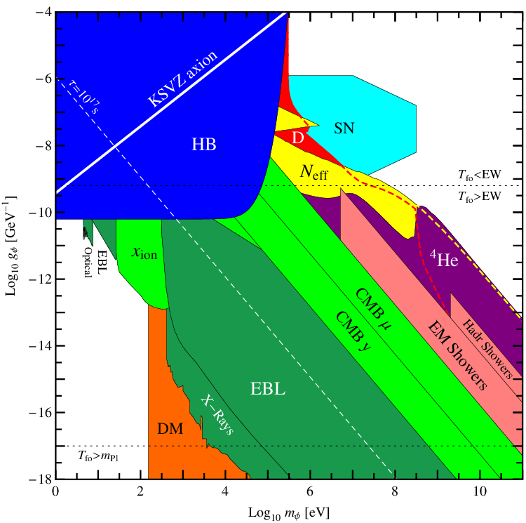
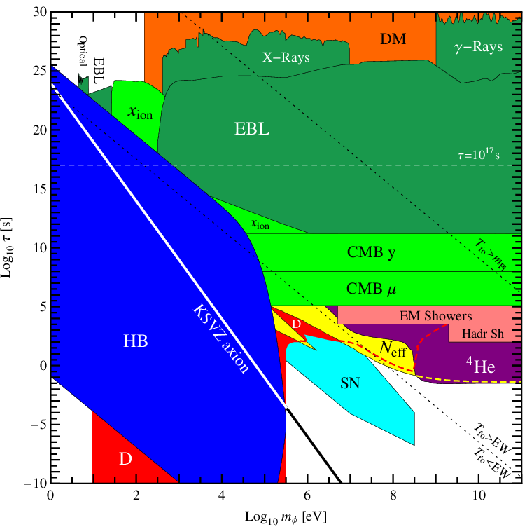
In our summary plots 5.1 and 5.2 we collected all the bounds arising from cosmology, considering a thermal origin for the primordial pseudoscalar population. While figure 5.1 is meant to be the reference for the particle physicist, since the ALP parameter space is plotted in function of the ALP mass and coupling , figure 5.2, where the parameters are and the lifetime , provides a better physical understanding. In this picture we can better follow the relation of the limits with the sequence of events in the history of the universe. The cosmological bounds critically depend on the ALP lifetime while they have only a milder dependence on other parameters. In figure 5.1 they have indeed the characteristic slope . As a reference, we plotted the line along which ALPs have the lifetime equal to s, i.e. the age of the universe. To warn the reader about our assumptions, we also plotted the lines for freezing out temperature equal to the electroweakscale and the Planck scale . Most likely, makes no physical sense, and for the actual abundance could be lower than that used in our calculations, since we have not taken into account other particles besides the ALP and the SM ones.
Ordered by decreasing lifetimes, the excluded regions are:
- •
DM — if ALPs are cosmologically stable and behave as dark matter they should not exceed the DM fraction measured by WMAP.
- •
Optical, X-Rays, -Rays — photons produced in pseudoscalar decays inside galaxies would show up as a peak in galactic spectra that must not exceed the known backgrounds.
- •
EBL — photons produced in pseudoscalar decays when the universe is transparent must not exceed the extragalactic background light.
- •
— the ionization of primordial hydrogen caused by the decay photons must not contribute significantly to the optical depth after recombination.
- •
CMB y, — if the decay happens when the universe is opaque, the decay photons must not cause spectral distortions in the CMB spectrum that cannot be fully rethermalised.
- •
EM, Hadr showers — the decay of high mass ALPs produces electromagnetic and hadronic showers that must not spoil the agreement of big-bang nucleosynthesis with observations of primordial nuclei.
- •
4He, D — the ALP and axion decays produce photons that dilute the baryon and neutrino densities, whose values affect the outcome of BBN, in particular the deuterium and 4He yields. Again, this dilution should not compromise BBN.
- •
— the neutrino density must not disagree with the value measured by WMAP and other large-scale-structure probes. Currently, data points to an effective number of neutrinos greater than 3, which is disfavoured in the cosmology of decaying pseudoscalars.
We have seen how cosmological observations can exclude a large part of the pseudoscalar parameter space. These limits are solid, and the prospects are good, since the amount and quality of cosmological observations is steeply rising. This is very important, since the constrained region lies in a part of the parameter space presently inaccessible to direct experimental tests.
The investigation on the effects of axions and ALPs on astrophysical and cosmological observables must proceed further, because the detection of one of several striking signatures could lead to their discovery. The smoking gun could be hidden in the white-dwarf evolution or in the structure of galaxies, maybe influenced by the dark matter in a Bose-Einstein condensate, or in some different phenomena that we still have to analyse. But after the eventual and desired discovery, the direct detection and laboratory experiments will have the task of measuring precisely the new particle characteristics. In the near future, direct detection experiments like the haloscopes and the helioscopes will finally reach the sensitivity to test the axion hypothesis and to explore two phenomenologically important regions of the parameter space, and maybe some long standing questions will find an answer.
Understanding the ultimate theory behind the laws of Nature is the final purpose of physics. The large hadron collider is pushing the knowledge on particle physics towards unexplored energy scales. The recent discovery of the Higgs boson gives a bit more confidence about the axion theory, which requires the existence of scalar fields and the spontaneous breaking of symmetries at high energy scales. But increasing the energy tested by colliders is not the only way to probe the physics beyond the SM. If axions and ALPs will be finally discovered, we will have the tempting possibility of exploring the physics related to very high energy scales through its low energy regime. Still largely unexplored, the low energy frontier could hide important novelties and bring to fundamental advances in the understanding of Nature.
Appendix A Axion-photon mixing
In the following we follow the treatment of [168] and [169], where the hidden photon resonance case was studied. The Lagrangian of the pseudoscalar-photon system in presence of a strong magnetic field , whose modulus is , is
| (A.1) |
where we expressed as the scalar product of the external magnetic field and of the electric field component of the field strength. From the Lagrangian we obtain the equations of motions for the pseudoscalar field and the component of the vector potential parallel to the magnetic field
| (A.2a) | ||||
| (A.2b) | ||||
while the perpendicular component is not affected by the interaction with . In equation (A.2a) we have used Ohm’s law for the current density, , assuming a linear response of the medium whose conductivity is [125]. In Fourier space the equations (A.2) become
| (A.3a) | ||||
| (A.3b) | ||||
Assuming the quantity to be negligible with respect to the other energy scales of the problem, this system of equations can be diagonalised by means of the redefinitions
| (A.4a) | |||
| (A.4b) | |||
The new states and are decoupled, and if the mixing parameter
| (A.5) |
is very small, they are almost photon and pseudoscalar states. They can oscillate one into another, if . Their dispersion relations are respectively
| (A.6a) | ||||
| (A.6b) | ||||
where the factors are complex. In the case of zero mode DM scalars, . The original states and can be obtained inserting the and solutions into the (A.4).
For the conductivity of the medium we use the relation [3]
| (A.7) |
that provides an interpolation of the classical approximation and the quantum regime. In this formula, is the plasma frequency and is the photon absorption width due to Thomson scattering off electrons, while is the average time between electron collisions, which sets the time scale. If we call and the momentum and the energy of electrons, the plasma frequency is [46]
| (A.8) |
We next define the squared plasmon mass
| (A.9) |
The damping factor
| (A.10) |
expresses the net-rate at which photons are created or absorbed. The full expressions for these quantities can be found in [168]. Using these definitions, the oscillation probability (A.5) becomes
| (A.11) |
Because of this magnetic field-mediated mixing with the photon, the pseudoscalar field has the same interactions of the photon, but with a rate suppressed by . In particular, it can be absorbed or emitted during Thomson-like interactions and annihilations-like events . If thermal contact is regained by the pseudoscalar condensate, its distribution tends towards equilibrium. The amount of pseudoscalars that survives the magnetic field induced evaporation is provided by
| (A.12) |
where the subscripts means quantities measured just after the realignment mechanism ended and are today quantities. We used in the integral the damping factor , that provides the net-rate of absorbed photons. Because we deal with temperature-depending quantities, for future convenience we can write the integral in the exponential of equation (A.12) as
| (A.13) |
The primordial magnetic field evolves with time, since it is stretched by the expansion of the universe. The conservation of magnetic flux implies , where the subscript refers to quantities measured at the reference time , after the creation of the primordial magnetic field at .
The temperature dependence of the conductivity (A.7) is mainly affected by . For the conductivity is dominated by the damping factor, thus if also . The damping factor is in a relativistic plasma of electrons [125], and equation (A.13) becomes
| (A.14) |
For axion cold DM this is the approximation to use, because the axion mass is much lower than the damping factor [125]. Axion cold DM is not affected by primordial magnetic field: its two photon coupling strength is much lower than , while the present value of the magnetic field can not be stronger than few nG [126, 127]. Even if is very large, it cannot affect the condensate at temperatures larger than , because in this case there is no condensate. Moreover, in the case of the hadronic axion, there is no two-photon coupling above .
When the damping factor does not suppress and it is much smaller in magnitude than the plasmon mass, we can distinguish three different regimes of this quantity, according to the relative magnitude between and . The resonant regime for is the most important, since the mixing gets enhanced by the cancellation of the mass terms in the denominator.

At temperatures higher than the resonant one, equation (A.13) is
| (A.15) |
which in both cases is dominated by lower temperatures, so towards the resonance. For the low temperature we used the conductivity provided by a hydrogen plasma [125]. The low temperature regime gives instead
| (A.16) |
which is dominated by the higher temperatures again towards the resonance. The behaviour of the integrand can even better understood from figure A.1, where this quantity is plotted for , 1 and 10 eV. Since this function is so peaked around the resonance, we can approximate the integral evaluating all the temperature dependent quantities around , expanding , and neglecting the rest
| (A.17) |
To obtain the last line we used the approximation
| (A.18) |
and . The pseudoscalar population is affected by the resonant magnetic field evaporation if the value of the integral (A.17) is larger than one. This is plotted in figure 2.10.
References
- [1] D. Cadamuro, S. Hannestad, G. Raffelt and J. Redondo, Cosmological bounds on sub-MeV mass axions, JCAP 1102 (2011) 003 [arXiv:1011.3694].
- [2] D. Cadamuro and J. Redondo, Cosmological bounds on pseudo Nambu-Goldstone bosons, JCAP 1202 (2012) 032 [arXiv:1110.2895].
- [3] P. Arias, D. Cadamuro, M. Goodsell, J. Jäckel, J. Redondo and A. Ringwald, WISPy cold dark matter, JCAP 1206 (2012) 013 [arXiv:1201.5902].
- [4] R. Peccei, The strong CP problem and axions, Lect. Notes Phys. 741 (2008) 3–17 [hep-ph/0607268].
- [5] J. E. Kim, Light pseudoscalars, particle physics and cosmology, Phys. Rept. 150 (1987) 1–177.
- [6] H.-Y. Cheng, The strong CP problem revisited, Phys. Rept. 158 (1988) 1.
- [7] J. E. Kim and G. Carosi, Axions and the strong CP problem, Rev. Mod. Phys. 82 (2010) 557–602 [arXiv:0807.3125].
- [8] G. ’t Hooft, Symmetry breaking through Bell-Jackiw anomalies, Phys. Rev. Lett. 37 (1976) 8–11.
- [9] G. ’t Hooft, Computation of the quantum effects due to a four-dimensional pseudoparticle, Phys. Rev. D14 (1976) 3432–3450.
- [10] J. Callan, Curtis G., R. Dashen and D. J. Gross, The structure of the gauge theory vacuum, Phys. Lett. B63 (1976) 334–340.
- [11] V. Baluni, CP violating effects in QCD, Phys. Rev. D19 (1979) 2227–2230.
- [12] R. Crewther, P. Di Vecchia, G. Veneziano and E. Witten, Chiral estimate of the electric dipole moment of the neutron in quantum chromodynamics, Phys. Lett. B88 (1979) 123.
- [13] C. Baker, D. Doyle, P. Geltenbort, K. Green, M. van der Grinten et. al., An improved experimental limit on the electric dipole moment of the neutron, Phys. Rev. Lett. 97 (2006) 131801 [hep-ex/0602020].
- [14] R. Peccei and H. R. Quinn, CP conservation in the presence of instantons, Phys. Rev. Lett. 38 (1977) 1440–1443.
- [15] R. Peccei and H. R. Quinn, Constraints imposed by CP conservation in the presence of instantons, Phys. Rev. D16 (1977) 1791–1797.
- [16] S. Weinberg, A new light boson?, Phys. Rev. Lett. 40 (1978) 223–226.
- [17] F. Wilczek, Problem of strong P and T invariance in the presence of instantons, Phys. Rev. Lett. 40 (1978) 279–282.
- [18] C. Vafa and E. Witten, Parity conservation in QCD, Phys. Rev. Lett. 53 (1984) 535.
- [19] S. Weinberg, The U(1) problem, Phys. Rev. D11 (1975) 3583–3593.
- [20] S. Weinberg, The quantum theory of fields. Vol. 2: Modern applications. Cambridge University Press, Cambridge, UK, 1996.
- [21] W. A. Bardeen and S.-H. Tye, Current algebra applied to properties of the light Higgs Boson, Phys. Lett. B74 (1978) 229.
- [22] Particle Data Group Collaboration, K. Nakamura et. al., Review of particle physics, J. Phys. G G37 (2010) 075021.
- [23] J. R. Ellis and M. K. Gaillard, No new light boson?, Phys. Lett. B74 (1978) 374.
- [24] J. E. Kim, Weak interaction singlet and strong CP invariance, Phys. Rev. Lett. 43 (1979) 103.
- [25] M. A. Shifman, A. Vainshtein and V. I. Zakharov, Can confinement ensure natural CP invariance of strong interactions?, Nucl. Phys. B166 (1980) 493.
- [26] A. Zhitnitsky, On possible suppression of the axion hadron interactions., Sov. J. Nucl. Phys. 31 (1980) 260.
- [27] M. Dine, W. Fischler and M. Srednicki, A simple solution to the strong CP problem with a harmless axion, Phys. Lett. B104 (1981) 199.
- [28] H. Georgi, D. B. Kaplan and L. Randall, Manifesting the invisible axion at low-energies, Phys. Lett. B169 (1986) 73.
- [29] P. Sikivie, Experimental tests of the invisible axion, Phys. Rev. Lett. 51 (1983) 1415.
- [30] E. Massó and R. Toldrà, On a light spinless particle coupled to photons, Phys. Rev. D52 (1995) 1755–1763 [hep-ph/9503293].
- [31] E. Massó and R. Toldrà, New constraints on a light spinless particle coupled to photons, Phys. Rev. D55 (1997) 7967–7969 [hep-ph/9702275].
- [32] F. Wilczek, Axions and family symmetry breaking, Phys. Rev. Lett. 49 (1982) 1549–1552.
- [33] Y. Chikashige, R. N. Mohapatra and R. Peccei, Spontaneously broken lepton number and cosmological constraints on the neutrino mass spectrum, Phys. Rev. Lett. 45 (1980) 1926.
- [34] Y. Chikashige, R. N. Mohapatra and R. Peccei, Are there real Goldstone bosons associated with broken lepton number?, Phys. Lett. B98 (1981) 265.
- [35] E. Chun, J. E. Kim and H. P. Nilles, A Natural solution of the mu problem with a composite axion in the hidden sector, Nucl. Phys. B370 (1992) 105–122.
- [36] A. E. Nelson and N. Seiberg, R symmetry breaking versus supersymmetry breaking, Nucl. Phys. B416 (1994) 46–62 [hep-ph/9309299].
- [37] P. Svrcek and E. Witten, Axions in string theory, JHEP 0606 (2006) 051 [hep-th/0605206].
- [38] M. A. Bershady, M. Ressell and M. S. Turner, Telescope search for multi-eV axions, Phys. Rev. Lett. 66 (1991) 1398–1401.
- [39] M. Ressell, Limits to the radiative decay of the axion, Phys. Rev. D44 (1991) 3001–3020.
- [40] J. M. Overduin and P. Wesson, Dark matter and background light, Phys. Rept. 402 (2004) 267–406 [astro-ph/0407207].
- [41] D. Grin, G. Covone, J.-P. Kneib, M. Kamionkowski, A. Blain et. al., A telescope search for decaying relic axions, Phys. Rev. D75 (2007) 105018 [astro-ph/0611502].
- [42] S. J. Asztalos, R. Bradley, L. Duffy, C. Hagmann, D. Kinion et. al., An improved RF cavity search for halo axions, Phys. Rev. D69 (2004) 011101 [astro-ph/0310042].
- [43] D. Lyapustin, The Axion Dark Matter eXperiment, [arXiv:1112.1167].
- [44] S. Asztalos, G. Carosi, C. Hagmann, D. Kinion, K. van Bibber et. al., Design and performance of the ADMX SQUID-based microwave receiver, Nucl. Instrum. Meth. A656 (2011) 39–44 [arXiv:1105.4203].
- [45] G. Carosi, ADMX Phase II+, Talk given at Vistas in Axion Physics workshop (April 2012) [http://www.int.washington.edu/talks/WorkShops/int_12_50W/People/Carosi_G/Carosi.pdf].
- [46] G. Raffelt, Stars as laboratories for fundamental physics: The astrophysics of neutrinos, axions, and other weakly interacting particles. University of Chicago Press, Chicago IL, US, 1996.
- [47] G. Raffelt and L. Stodolsky, Mixing of the photon with low mass particles, Phys. Rev. D37 (1988) 1237.
- [48] A. Halprin, C. Andersen and H. Primakoff, Photonic decay rates and nuclear-Coulomb-field coherent production processes, Phys. Rev. 152 (1966) 1295–1303.
- [49] G. G. Raffelt, Astrophysical axion bounds, Lect. Notes Phys. 741 (2008) 51–71 [hep-ph/0611350].
- [50] Y. Inoue, Y. Akimoto, R. Ohta, T. Mizumoto, A. Yamamoto et. al., Search for solar axions with mass around 1 eV using coherent conversion of axions into photons, Phys. Lett. B668 (2008) 93–97 [arXiv:0806.2230].
- [51] CAST Collaboration, S. Aune et. al., CAST search for sub-eV mass solar axions with 3He buffer gas, Phys. Rev. Lett. 107 (2011) 261302 [arXiv:1106.3919].
- [52] IAXO Collaboration, I. Irastorza et. al., The International Axion Observatory (IAXO), [arXiv:1201.3849].
- [53] J. Engel, D. Seckel and A. Hayes, Emission and detectability of hadronic axions from SN1987A, Phys. Rev. Lett. 65 (1990) 960–963.
- [54] E. Riordan, M. Krasny, K. Lang, P. De Barbaro, A. Bodek et. al., A search for short lived axions in an electron beam dump experiment, Phys. Rev. Lett. 59 (1987) 755.
- [55] J. Bjorken, S. Ecklund, W. Nelson, A. Abashian, C. Church et. al., Search for neutral metastable penetrating particles produced in the SLAC beam dump, Phys. Rev. D38 (1988) 3375.
- [56] J. Jäckel and A. Ringwald, The low-energy frontier of particle physics, Ann. Rev. Nucl. Part. Sci. 60 (2010) 405–437 [arXiv:1002.0329].
- [57] J. Redondo and A. Ringwald, Light shining through walls, Contemp. Phys. 52 (2011) 211–236 [arXiv:1011.3741].
- [58] K. Ehret, M. Frede, S. Ghazaryan, M. Hildebrandt, E.-A. Knabbe et. al., New ALPS results on hidden-sector lightweights, Phys. Lett. B689 (2010) 149–155 [arXiv:1004.1313].
- [59] L. Maiani, R. Petronzio and E. Zavattini, Effects of nearly massless, spin zero particles on light propagation in a magnetic field, Phys. Lett. B175 (1986) 359.
- [60] R. Battesti, B. Beltran, H. Davoudiasl, M. Kuster, P. Pugnat et. al., Axion searches in the past, at present, and in the near future, Lect. Notes Phys. 741 (2008) 199–237 [arXiv:0705.0615].
- [61] J. S. Schwinger, On gauge invariance and vacuum polarization, Phys. Rev. 82 (1951) 664–679.
- [62] S. L. Adler, Photon splitting and photon dispersion in a strong magnetic field, Annals Phys. 67 (1971) 599–647.
- [63] PVLAS Collaboration, E. Zavattini et. al., New PVLAS results and limits on magnetically induced optical rotation and ellipticity in vacuum, Phys. Rev. D77 (2008) 032006 [arXiv:0706.3419].
- [64] R. Gill and J. S. Heyl, Constraining the photon-axion coupling constant with magnetic white dwarfs, Phys. Rev. D84 (2011) 085001 [arXiv:1105.2083].
- [65] H.E.S.S. Collaboration, F. Aharonian et. al., A low level of extragalactic background light as revealed by gamma-rays from blazars, Nature 440 (2006) 1018–1021 [astro-ph/0508073].
- [66] D. Mazin and M. Raue, New limits on the density of the extragalactic background light in the optical to the far-infrared from the spectra of all known TeV blazars, Astron. Astrophys. 471 (2007) 439–452 [astro-ph/0701694].
- [67] A. De Angelis, O. Mansutti and M. Roncadelli, Evidence for a new light spin-zero boson from cosmological gamma-ray propagation?, Phys.Rev. D76 (2007) 121301 [arXiv:0707.4312].
- [68] D. Hooper and P. D. Serpico, Detecting axion-like particles with gamma ray telescopes, Phys. Rev. Lett. 99 (2007) 231102 [arXiv:0706.3203].
- [69] K. A. Hochmuth and G. Sigl, Effects of axion-photon mixing on gamma-ray spectra from magnetized astrophysical sources, Phys. Rev. D76 (2007) 123011 [arXiv:0708.1144].
- [70] M. Simet, D. Hooper and P. D. Serpico, The Milky Way as a kiloparsec-scale axionscope, Phys. Rev. D77 (2008) 063001 [arXiv:0712.2825].
- [71] D. Horns, L. Maccione, M. Meyer, A. Mirizzi, D. Montanino et. al., Hardening of TeV gamma spectrum of AGNs in galaxy clusters by conversions of photons into axion-like particles, [arXiv:1207.0776].
- [72] N. Bassan, A. Mirizzi and M. Roncadelli, Axion-like particle effects on the polarization of cosmic high-energy gamma sources, JCAP 1005 (2010) 010 [arXiv:1001.5267].
- [73] D. Horns, L. Maccione, A. Mirizzi and M. Roncadelli, Probing axion-like particles with the ultraviolet photon polarization from active galactic nuclei in radio galaxies, Phys.Rev. D85 (2012) 085021 [arXiv:1203.2184].
- [74] A. Payez, J. Cudell and D. Hutsemekers, New polarimetric constraints on axion-like particles, JCAP 1207 (2012) 041 [arXiv:1204.6187].
- [75] J. Isern, E. Garcia-Berro, S. Torres and S. Catalan, Axions and the cooling of white dwarf stars, Astrophys. J. L. 682 (2008) L109 [arXiv:0806.2807].
- [76] E. W. Kolb and M. S. Turner, The Early universe. Westview Press, Boulder CO, US, 1990.
- [77] M. Dine and W. Fischler, The not so harmless axion, Phys. Lett. B120 (1983) 137–141.
- [78] L. Abbott and P. Sikivie, A cosmological bound on the invisible axion, Phys. Lett. B120 (1983) 133–136.
- [79] J. Preskill, M. B. Wise and F. Wilczek, Cosmology of the invisible axion, Phys. Lett. B120 (1983) 127–132.
- [80] A. Arvanitaki, S. Dimopoulos, S. Dubovsky, N. Kaloper and J. March-Russell, String axiverse, Phys. Rev. D81 (2010) 123530 [arXiv:0905.4720].
- [81] B. S. Acharya, K. Bobkov and P. Kumar, An M theory solution to the strong CP problem and constraints on the axiverse, JHEP 1011 (2010) 105 [arXiv:1004.5138].
- [82] D. J. Marsh, The axiverse extended: vacuum destabilisation, early dark energy and cosmological collapse, Phys. Rev. D83 (2011) 123526 [arXiv:1102.4851].
- [83] T. Higaki and T. Kobayashi, Note on moduli stabilization, supersymmetry breaking and axiverse, Phys. Rev. D84 (2011) 045021 [arXiv:1106.1293].
- [84] E. Massó, F. Rota and G. Zsembinszki, Planck-scale effects on global symmetries: Cosmology of pseudo-Goldstone bosons, Phys. Rev. D70 (2004) 115009 [hep-ph/0404289].
- [85] A. E. Nelson and J. Scholtz, Dark light, dark matter and the misalignment mechanism, Phys. Rev. D84 (2011) 103501 [arXiv:1105.2812].
- [86] WMAP Collaboration, E. Komatsu et. al., Seven-year Wilkinson microwave anisotropy probe (WMAP) observations: cosmological interpretation, Astrophys. J. Suppl. 192 (2011) 18 [arXiv:1001.4538].
- [87] P. Sikivie and Q. Yang, Bose-Einstein condensation of dark matter axions, Phys. Rev. Lett. 103 (2009) 111301 [arXiv:0901.1106].
- [88] O. Erken, P. Sikivie, H. Tam and Q. Yang, Cosmic axion thermalization, Phys. Rev. D85 (2012) 063520 [arXiv:1111.1157].
- [89] L. Duffy and P. Sikivie, The caustic ring model of the milky way halo, Phys. Rev. D78 (2008) 063508 [arXiv:0805.4556].
- [90] B. Kain and H. Y. Ling, Cosmological inhomogeneities with Bose-Einstein condensate dark matter, Phys. Rev. D85 (2012) 023527 [arXiv:1112.4169].
- [91] D. J. Gross, R. D. Pisarski and L. G. Yaffe, QCD and instantons at finite temperature, Rev. Mod. Phys. 53 (1981) 43.
- [92] O. Wantz and E. Shellard, Axion cosmology revisited, Phys. Rev. D82 (2010) 123508 [arXiv:0910.1066].
- [93] M. P. Hertzberg, M. Tegmark and F. Wilczek, Axion cosmology and the energy scale of inflation, Phys. Rev. D78 (2008) 083507 [arXiv:0807.1726].
- [94] J. Hamann, S. Hannestad, G. G. Raffelt and Y. Y. Wong, Isocurvature forecast in the anthropic axion window, JCAP 0906 (2009) 022 [arXiv:0904.0647].
- [95] S. Hannestad, What is the lowest possible reheating temperature?, Phys. Rev. D70 (2004) 043506 [astro-ph/0403291].
- [96] W. Büchmuller, P. Di Bari and M. Plümacher, Leptogenesis for pedestrians, Annals Phys. 315 (2005) 305–351 [hep-ph/0401240].
- [97] K. J. Mack, Axions, inflation and the anthropic principle, JCAP 1107 (2011) 021 [arXiv:0911.0421].
- [98] M. Tegmark, A. Aguirre, M. Rees and F. Wilczek, Dimensionless constants, cosmology and other dark matters, Phys. Rev. D73 (2006) 023505 [astro-ph/0511774].
- [99] C. Hogan and M. Rees, Axion miniclusters, Phys. Lett. B205 (1988) 228–230.
- [100] E. W. Kolb and I. I. Tkachev, Axion miniclusters and Bose stars, Phys. Rev. Lett. 71 (1993) 3051–3054 [hep-ph/9303313].
- [101] E. W. Kolb and I. I. Tkachev, Nonlinear axion dynamics and formation of cosmological pseudosolitons, Phys. Rev. D49 (1994) 5040–5051 [astro-ph/9311037].
- [102] K. M. Zurek, C. J. Hogan and T. R. Quinn, Astrophysical effects of scalar dark matter miniclusters, Phys. Rev. D75 (2007) 043511 [astro-ph/0607341].
- [103] E. W. Kolb and I. I. Tkachev, Femtolensing and picolensing by axion miniclusters, Astrophys. J. 460 (1996) L25–L28 [astro-ph/9510043].
- [104] A. Vilenkin and A. Everett, Cosmic strings and domain walls in models with Goldstone and pseudo-Goldstone bosons, Phys. Rev. Lett. 48 (1982) 1867–1870.
- [105] D. Harari and P. Sikivie, On the evolution of global strings in the early universe, Phys. Lett. B195 (1987) 361.
- [106] C. Hagmann and P. Sikivie, Computer simulations of the motion and decay of global strings, Nucl. Phys. B363 (1991) 247–280.
- [107] R. L. Davis, Goldston bosons in string models of galaxy formation, Phys. Rev. D32 (1985) 3172.
- [108] R. L. Davis, Cosmic axions from cosmic strings, Phys. Lett. B180 (1986) 225.
- [109] A. Vilenkin and T. Vachaspati, Radiation of Goldstone bosons from cosmic strings, Phys. Rev. D35 (1987) 1138.
- [110] R. Davis and E. Shellard, Do axions need inflation?, Nucl. Phys. B324 (1989) 167.
- [111] A. Dabholkar and J. M. Quashnock, Pinning down the axion, Nucl. Phys. B333 (1990) 815.
- [112] R. Battye and E. Shellard, Global string radiation, Nucl. Phys. B423 (1994) 260–304 [astro-ph/9311017].
- [113] R. Battye and E. Shellard, Axion string constraints, Phys. Rev. Lett. 73 (1994) 2954–2957 [astro-ph/9403018].
- [114] P. Sikivie, Of axions, domain walls and the early universe, Phys. Rev. Lett. 48 (1982) 1156–1159.
- [115] T. Hiramatsu, M. Kawasaki, K. Saikawa and T. Sekiguchi, Production of dark matter axions from collapse of string-wall systems, Phys. Rev. D85 (2012) 105020 [arXiv:1202.5851].
- [116] G. Carosi and K. van Bibber, Cavity microwave searches for cosmological axions, Lect. Notes Phys. 741 (2008) 135–156 [hep-ex/0701025].
- [117] W. Wuensch, S. De Panfilis-Wuensch, Y. Semertzidis, J. Rogers, A. Melissinos et. al., Results of a laboratory search for cosmic axions and other weakly coupled light particles, Phys. Rev. D40 (1989) 3153.
- [118] C. Hagmann, P. Sikivie, N. Sullivan and D. Tanner, Results from a search for cosmic axions, Phys. Rev. D42 (1990) 1297–1300.
- [119] P. Gondolo and G. Gelmini, Cosmic abundances of stable particles: improved analysis, Nucl. Phys. B360 (1991) 145–179.
- [120] P. Graf and F. D. Steffen, Thermal axion production in the primordial quark-gluon plasma, Phys. Rev. D83 (2011) 075011 [arXiv:1008.4528].
- [121] S. Hannestad, A. Mirizzi and G. Raffelt, New cosmological mass limit on thermal relic axions, JCAP 0507 (2005) 002 [hep-ph/0504059].
- [122] S. Hannestad, A. Mirizzi, G. G. Raffelt and Y. Y. Wong, Neutrino and axion hot dark matter bounds after WMAP-7, JCAP 1008 (2010) 001 [arXiv:1004.0695].
- [123] M. Bolz, A. Brandenburg and W. Büchmuller, Thermal production of gravitinos, Nucl. Phys. B606 (2001) 518–544 [hep-ph/0012052].
- [124] D. Grasso and H. R. Rubinstein, Magnetic fields in the early universe, Phys. Rept. 348 (2001) 163–266 [astro-ph/0009061].
- [125] J. Ahonen, K. Enqvist and G. Raffelt, The paradox of axions surviving primordial magnetic fields, Phys. Lett. B366 (1996) 224–228 [hep-ph/9510211].
- [126] T. Kahniashvili, A. G. Tevzadze, S. K. Sethi, K. Pandey and B. Ratra, Primordial magnetic field limits from cosmological data, Phys. Rev. D82 (2010) 083005 [arXiv:1009.2094].
- [127] D. Paoletti and F. Finelli, CMB constraints on a stochastic background of primordial magnetic fields, Phys. Rev. D83 (2011) 123533 [arXiv:1005.0148].
- [128] W. Hu and J. Silk, Thermalization and spectral distortions of the cosmic background radiation, Phys. Rev. D48 (1993) 485–502.
- [129] D. Fixsen, E. Cheng, J. Gales, J. C. Mather, R. Shafer et. al., The Cosmic Microwave Background spectrum from the full COBE FIRAS data set, Astrophys. J. 473 (1996) 576 [astro-ph/9605054].
- [130] Y. B. Zeldovich and R. A. Sunyaev, The interaction of matter and radiation in a hot-model Universe, Astrophys. Space Sci. 4 (1969) 301.
- [131] P. J. E. Peebles, Principles of physical cosmology. Princeton University Press, Princeton NJ, US, 1993.
- [132] V. Mukhanov, Physical foundations of cosmology. Cambridge University Press, Cambridge, UK, 2005.
- [133] T. R. Choudhury and A. Ferrara, Physics of cosmic reionization, [astro-ph/0603149].
- [134] A. Natarajan and D. J. Schwarz, Distinguishing standard reionization from dark matter models, Phys. Rev. D81 (2010) 123510 [arXiv:1002.4405].
- [135] S. Seager, D. D. Sasselov and D. Scott, A new calculation of the recombination epoch, Astrophys. J. 523 (1999) L1–L5 [astro-ph/9909275].
- [136] B. Bransden and C. Joachain, Physics of atoms and molecules. Pearson Education. Prentice Hall, Harlow, UK, 2003.
- [137] E. Massó and R. Toldrà, Photon spectrum produced by the late decay of a cosmic neutrino background, Phys. Rev. D60 (1999) 083503 [astro-ph/9903397].
- [138] A. Boyarsky, A. Neronov, O. Ruchayskiy, M. Shaposhnikov and I. Tkachev, Where to find a dark matter sterile neutrino?, Phys. Rev. Lett. 97 (2006) 261302 [astro-ph/0603660].
- [139] A. Boyarsky, O. Ruchayskiy and M. Shaposhnikov, The role of sterile neutrinos in cosmology and astrophysics, Ann. Rev. Nucl. Part. Sci. 59 (2009) 191–214 [arXiv:0901.0011].
- [140] G. Vertongen and C. Weniger, Hunting dark matter gamma-ray lines with the Fermi LAT, JCAP 1105 (2011) 027 [arXiv:1101.2610].
- [141] C. Weniger, A tentative gamma-ray line from dark matter annihilation at the Fermi Large Area Telescope, JCAP 1208 (2012) 007 [arXiv:1204.2797].
- [142] G. Mangano, G. Miele, S. Pastor, T. Pinto, O. Pisanti et. al., Relic neutrino decoupling including flavor oscillations, Nucl. Phys. B729 (2005) 221–234 [hep-ph/0506164].
- [143] J. Hamann, S. Hannestad, G. Raffelt and Y. Y. Wong, Observational bounds on the cosmic radiation density, JCAP 0708 (2007) 021 [arXiv:0705.0440].
- [144] J. Hamann, S. Hannestad, J. Lesgourgues, C. Rampf and Y. Y. Wong, Cosmological parameters from large scale structure - geometric versus shape information, JCAP 1007 (2010) 022 [arXiv:1003.3999].
- [145] M. Gonzalez-Garcia, M. Maltoni and J. Salvado, Robust cosmological bounds on neutrinos and their combination with oscillation results, JHEP 1008 (2010) 117 [arXiv:1006.3795].
- [146] J. Hamann, S. Hannestad, G. G. Raffelt, I. Tamborra and Y. Y. Wong, Cosmology seeking friendship with sterile neutrinos, Phys. Rev. Lett. 105 (2010) 181301 [arXiv:1006.5276].
- [147] J. Hamann, J. Lesgourgues and G. Mangano, Using BBN in cosmological parameter extraction from CMB: a forecast for PLANCK, JCAP 0803 (2008) 004 [arXiv:0712.2826].
- [148] O. Pisanti, A. Cirillo, S. Esposito, F. Iocco, G. Mangano et. al., PArthENoPE: Public Algorithm Evaluating the Nucleosynthesis of Primordial Elements, Comput. Phys. Commun. 178 (2008) 956–971 [arXiv:0705.0290].
- [149] Y. Izotov and T. Thuan, The primordial abundance of 4He: evidence for non-standard big bang nucleosynthesis, Astrophys. J. 710 (2010) L67–L71 [arXiv:1001.4440].
- [150] G. Mangano and P. D. Serpico, A robust upper limit on from BBN, circa 2011, Phys. Lett. B701 (2011) 296–299 [arXiv:1103.1261].
- [151] M. Pettini, B. J. Zych, M. T. Murphy, A. Lewis and C. C. Steidel, Deuterium abundance in the most metal-poor damped Lyman alpha system: converging on , Mon. Not. Roy. Astron. Soc. 391 (2008) 1499–1510 [arXiv:0805.0594].
- [152] M. Fumagalli, J. M. O’Meara and J. X. Prochaska, Detection of pristine gas two billion years after the big bang, Science 334 (2011) 1245–1249 [arXiv:1111.2334].
- [153] R. H. Cyburt, B. D. Fields and K. A. Olive, An update on the big bang nucleosynthesis prediction for Li-7: The problem worsens, JCAP 0811 (2008) 012 [arXiv:0808.2818].
- [154] B. D. Fields, The primordial lithium problem, Ann. Rev. Nucl. Part. Sci. 61 (2011) 47–68 [arXiv:1203.3551].
- [155] V. F. Mukhanov, Nucleosynthesis without a computer, Int. J. Theor. Phys. 43 (2004) 669–693 [astro-ph/0303073].
- [156] R. Esmailzadeh, G. D. Starkman and S. Dimopoulos, Primordial nucleosynthesis without a computer, Astrophys. J. (1990).
- [157] A. Cuoco, F. Iocco, G. Mangano, G. Miele, O. Pisanti et. al., Present status of primordial nucleosynthesis after WMAP: results from a new BBN code, Int. J. Mod. Phys. A19 (2004) 4431–4454 [astro-ph/0307213].
- [158] K. A. Olive, G. Steigman and T. P. Walker, Primordial nucleosynthesis: theory and observations, Phys. Rept. 333 (2000) 389–407 [astro-ph/9905320].
- [159] S. Sarkar, Big bang nucleosynthesis and physics beyond the standard model, Rept. Prog. Phys. 59 (1996) 1493–1610 [hep-ph/9602260].
- [160] F. Iocco, G. Mangano, G. Miele, O. Pisanti and P. D. Serpico, Primordial nucleosynthesis: from precision cosmology to fundamental physics, Phys. Rept. 472 (2009) 1–76 [arXiv:0809.0631].
- [161] M. Pospelov and J. Pradler, Big bang nucleosynthesis as a probe of new physics, Ann. Rev. Nucl. Part. Sci. 60 (2010) 539–568 [arXiv:1011.1054].
- [162] R. H. Cyburt, J. R. Ellis, B. D. Fields and K. A. Olive, Updated nucleosynthesis constraints on unstable relic particles, Phys. Rev. D67 (2003) 103521 [astro-ph/0211258].
- [163] M. Kawasaki and T. Moroi, Electromagnetic cascade in the early universe and its application to the big bang nucleosynthesis, Astrophys. J. 452 (1995) 506 [astro-ph/9412055].
- [164] R. H. Cyburt, J. Ellis, B. D. Fields, F. Luo, K. A. Olive et. al., Nucleosynthesis constraints on a massive gravitino in neutralino dark matter scenarios, JCAP 0910 (2009) 021 [arXiv:0907.5003].
- [165] M. Kawasaki, K. Kohri and T. Moroi, Big-Bang nucleosynthesis and hadronic decay of long-lived massive particles, Phys. Rev. D71 (2005) 083502 [astro-ph/0408426].
- [166] M. Kawasaki, K. Kohri and T. Moroi, Hadronic decay of late-decaying particles and big bang nucleosynthesis, Phys. Lett. B625 (2005) 7–12 [astro-ph/0402490].
- [167] M. Reno and D. Seckel, Primordial nucleosynthesis: the effects of injecting hadrons, Phys. Rev. D37 (1988) 3441.
- [168] J. Redondo and M. Postma, Massive hidden photons as lukewarm dark matter, JCAP 0902 (2009) 005 [arXiv:0811.0326].
- [169] J. Redondo, Helioscope bounds on hidden sector photons, JCAP 0807 (2008) 008 [arXiv:0801.1527].
Acknowledgement
First of all, I would like to thank Dr. Javier Redondo and Dr. Georg Raffelt for their supervision of the Ph.D. project and the careful reading of this thesis. A big “thank you” is also for my collaborators, it has been a pleasure to work with them. In particular I want to thank Dr. Jörg Jäckel for reading the manuscript and giving me feedback.
I want to thank my office mates, Peter Graf and Dr. Srđan Sarikas, and my colleagues, for the nice conversations about physics and the world around us. Moreover, the German abstract would not have been in this shape if not for Peter. Special thanks go also to the “smokers & friends club”: Dr. Lorenzo Calibbi, Dr. Javier Redondo, Dr. Toshihiko Ota, Dr. Daniel Greenwald and Mr. Davide Pagani. They alleviated the fatigues of the work with nice and refreshing afternoon breaks.
Finally, I am very indebted to my wife Sara for her support, her patience and most of all her choice to follow me here to Munich. Thanks.