Scattering and bound states of two polaritons in an array of coupled cavities

In the recent years, the investigation of the physics in one-dimensional (1D) [1, 2, 3, 4, 5, 6, 7, 8, 9, 10, 11, 12, 13, 14, 15] and two-dimensional (2D) [14, 15, 16, 17, 18, 19, 20, 21, 22, 23] array of coupled cavities has attracted a lot of attention. It is predicted that, such systems can be used in quantum information processing [1, 2, 3, 4, 5] as well as the quantum simulation of many-body systems, e.g., the quantum phase simulation [14, 15, 10, 11, 13, 16, 17, 18, 19, 20, 12], quantum Hall effect [21] and Bose-Einstein condensate [22]. For the few-body physics of coupled cavities, many authors have studied the single-photon transmission in a 1D cavity array coupled with a single atom [1], and the dynamics of a single polariton in a 1D cavity array with each cavity coupled to an atom [2, 7]. Recently, bound states of two polaritons in such a system with finite number of cavities was studied by Wong and Law by direct numerical diagonalization of the Hamiltonian [8]. However, the scattering and bound states of two polaritons in an infinite array of coupled cavities remain to be investigated.

In this paper, we develop an analytical approach for calculating the scattering and bound states of two polaritons in an infinite array of coupled cavities with each cavity coupled to a two-level system (TLS), which can be either a natural or an artificial atom. In particular, we find that in such a system there is an effective contact interaction between two polaritons. Similarly to the photon blockade phenomenon [24], this effective interaction is also due to the nonlinearity of the Jaynes-Cummigs (JC) Hamiltonian. With our approach, one can treat the problem with standard techniques of quantum scattering. We further derive the scattering coefficient and bound-state energy of two polaritons with zero center-of-mass momentum. The resonance phenomena induced by the weakly bound states are also investigated. Our results can be directly used in the research of the transport of two polaritons. It is also helpful for the investigation of the many-body physics in a dilute gas of polaritons in a 1D cavity array.

This paper is organized as follows. In Sec. II we derive the effective interaction between two polaritons. Based on this result, the analytical method for calculating two-polariton scattering states and bound states is developed in Sec. III. In Sec. IV we solve the two-polariton problem with zero center-of-mass momentum with our approach and analyze the resonance phenomena. We conclude and discuss these results in Sec. V.

We consider a one-dimensional (1D) infinite array of coupled single-mode cavities. In each cavity there is a two-level system (TLS), which interacts with the photon in the cavity.

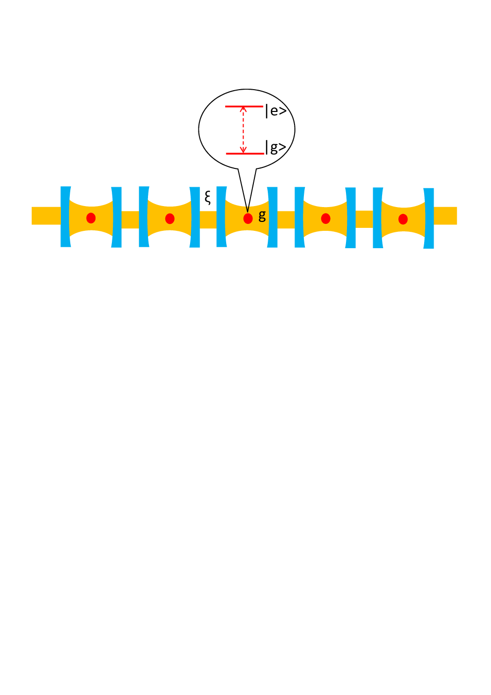
In the interaction picture, the Hamiltonian of the system is given by

where $\Delta=\omega_{A}-\omega_{L}$ is the detuning between the TLS and the cavity mode, with $\omega_{A}$ and $\omega_{L}$ the frequency of the TLS and the photon, respectively. In Eq. (1) $\xi$ is the hopping intensity or the inter-cavity coupling strength, $a_{n}$ and $a_{n}^{{\dagger}}$ are the annihilation and creation operators of the photons in the $n$-th cavity respectively, and $g$ is the coupling intensity between the TLS and the photon in the $n$-th cavity. Without loss of generality, here we assume that $g$ and $\xi$ are real numbers. The Pauli operator $\sigma_{ij}^{(n)}$ ($i,j=e,g$) is defined as $\sigma_{ij}^{(n)}=|i\rangle_{t}^{(n)}\langle j|$, with $|g\rangle_{t}^{(n)}$ and $|e\rangle_{t}^{(n)}$ the ground and excited state of the TLS in the $n$-th cavity, respectively. For the convenience of our following discussion, we further define $|0\rangle_{c}^{(n)}$ as the vacuum state of the $n$-th cavity.

We can define the “vacuum” state of our total system as

where all the atoms are in their ground level and there is no photon. Both the creation of photon and the excitation of TLS can be considered as the polaritons of the system. We can define the number operator of polaritons as

It is clear that $\left[H,N\right]=0$ and the polariton number is conserved. In case of $N=1$, there is a single polariton in our system, and Hamiltonian $H$ has eigen-states $A_{k}^{\dagger}|G\rangle$ or $B_{k}^{\dagger}|G\rangle$ with eigen-energies $\varepsilon_{Ak,Bk}=(2\xi\cos k+\Delta\pm\sqrt{(2\xi\cos k-\Delta)^{2}+4g^{2}})/2.$ Here

are the creation operators of the excitonic polariton of kind $A$ or $B$ with momentum $k$. The coefficients $\eta_{A,B}\left(k\right)$ and $\eta_{A,B}^{\prime}\left(k\right)$ can be obtained straightforwardly from the eigen-equaiton of $H$.

In this paper we consider the two-body problem of polaritons in our system, i.e., the quantum dynamics of our system in the subspace with $N=2$. In such a subspace, due to the translation symmetry of our system, the total momentum of the two polaritons is conserved, and thus the eigen-state of the Hamiltonian $H$ can be written as

with $K\in[-2\pi,2\pi)$ the total momentum of the two polaritons, and the coefficients $t_{l},d_{l},p_{l}$ describe the relative motion of the two polaritons, and satisfy

We can further define the coefficients $d_{l\pm}=\left(d_{l}\pm d_{-l}\right)/2$ which satisfy $d_{l\pm}=\pm d_{-l\pm}.$

It is apparent that the quantum state $|\Psi\rangle$ is described by a $4$-dimensional vector

which can be considered as the “spinor wave function” of the relative motion of two polaritons in the state $|\Psi\rangle$. Thus, the condition (6) for the coefficients can be re-expressed as

Here the matrix $\mathcal{T}$ is defined as

A straightforward calculation shows that, the eigenequation $H|\Psi\rangle=E|\Psi\rangle$ of the Hamiltonian $H$ can be re-written as

Here for each given value of $\left(l,l^{\prime}\right)$, $\mathbf{H}_{l,l^{\prime}}^{(0)}$ and $\mathbf{V}_{l,l^{\prime}}$ are $4$-dimensional matrixes and defined as

and

with the matrixes $\mathcal{A}$, $\mathcal{B}$ and $\mathcal{C}$ given by

The above discussion shows that the Schrödinger equation for the relative motion of two polaritons in our system is equivalent to Eq. (10) and the boundary condition (8) for the coefficient $\beta_{l}$. It is obvious that Eq. (10) has a same form as the stationary Schrödinger equation for a scattering problem. Then we can understand the matrix $\mathbf{H}_{l,l^{\prime}}^{(0)}$ as the “free-Hamiltonian” of the two-polariton relative motion, and $\mathbf{V}_{l,l^{\prime}}$ as the “interaction” between these two polaritons. Therefore, we can use the standard technique of quantum scattering problem to solve Eq. (10), and then find the scattering states and bound states of the two polaritons in our system.

Now we comment on the physical picture given by the inter-polariton interaction $\mathbf{V}_{l,l^{\prime}}$. It is clear that, the symbol $l\left(l^{\prime}\right)$ is an abbreviation of $m-n$ in Eq. (5), and thus describes the relative position of two polaritons. Since $\mathbf{V}_{l,l^{\prime}}$ takes non-zero value only when $l=l^{\prime}=0$, it is a two-polariton contact potential. Namely, two polaritons interact with each other when they are in the same cavity. To understand the physical meaning of this contact potential, we consider a extreme case where the photon cannot tunnel between different cavities. In that case, the total Hamiltonian becomes $H=\sum_{j=-\infty}^{\infty}H_{JC}^{(j)}$ with the JC Hamiltonian $H_{JC}^{(j)}=\Delta\sigma_{ee}^{(j)}+g\sigma_{eg}^{\left(j\right)}a_{j}+h.c.$. It is clear that $H_{JC}^{(n)}$ can be diagonalized in the subspace with $\sigma_{ee}^{(j)}+a_{j}^{\dagger}a_{j}=$ $n$ $(n=0,1,2...)$, and the relevant eigen-energies are $\varepsilon_{JC}^{(\pm)}(n)=(\Delta\pm\sqrt{\Delta^{2}+4g^{2}n})/2$. If two polaritons appear in two different cavities, the total energy of the two polaritons can take the ($i,j$)-independent value $\varepsilon_{JC}^{(\pm)}(1)+\varepsilon_{JC}^{(\pm)}(1)$. However, if the two polaritons appear in the same cavity, the energy of the two polaritons take the value $\varepsilon_{JC}^{(\pm)}(2)\neq\varepsilon_{JC}^{(\pm)}(1)+\varepsilon_{JC}^{(\pm)}(1)$. Therefore, due to the nonlinearity of the spectrum of JC Hamiltonian, the energy of two polaritons changes when they are in the same cavity. That is the origin of the effective contact interaction $\mathbf{V}_{l,l^{\prime}}$ of two polaritons in our system.

In the above section, we find that the two-polariton problem in the 1D cavity array is described by Eq. (10) with boundary condition (8). In this section we show our approach for solving Eq. (10) and derive the scattering states and bound states of two polaritons.

In the above section, we show our analytical approach for the calculations of two-polariton scattering states and bound states in a 1D cavity array. With our method, one can derive the scattering coefficient and bound states of two polaritons in the systems with any detuning $\Delta$ and coupling parameters $(g,\xi)$. Now we show the results of our calculations. For simplicity, in this paper we only consider case with the total momentum $K=0$.

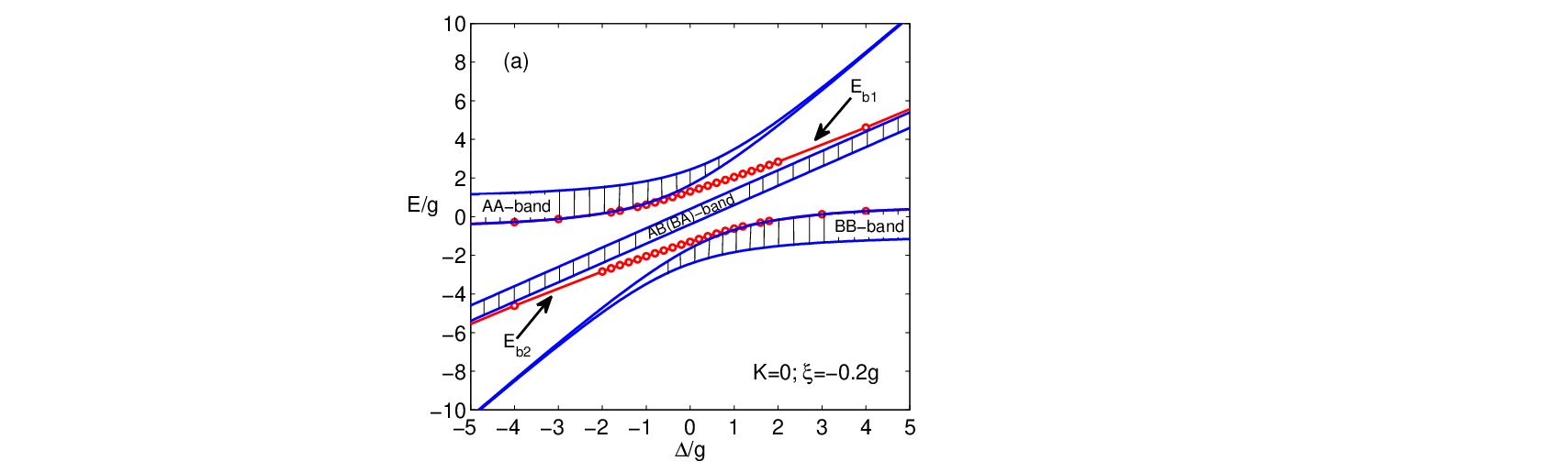
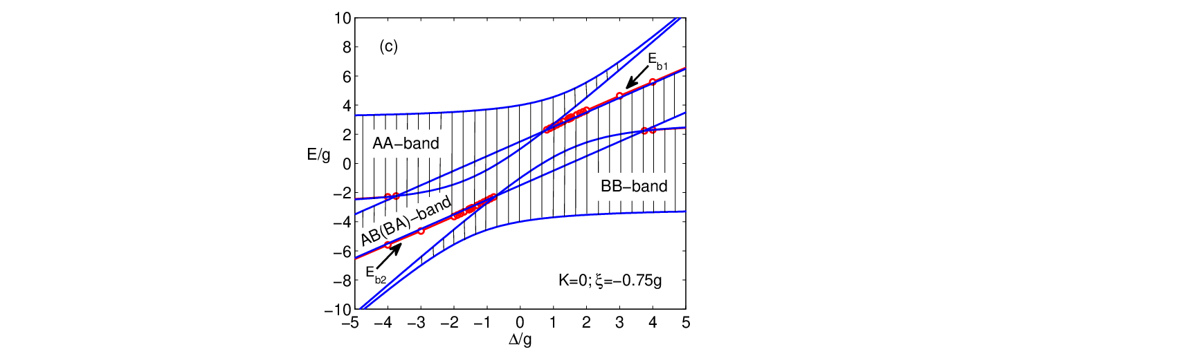
As discussed above, the energy of the two-polariton scattering state $\beta_{l}^{(+)}\left(uv,q\right)$ with $u,v=A,B$ is $E(uv,q)$ defined Eq. (30) . In the following, we call the region of value of $E(uv,q)$ with $q\in[-\pi,\pi)$ as “$uv$-band”. Then the energies of the scattering states are located in $AA$-, $AB$-, $BA$-, and $BB$-bands. Furthermore, we have $E(AB,q)=E(BA,-q)$. Thus the $AB$-band and $BA$-band totally overlap with each other, and we have three energy bands for the two-polariton scattering states. In Fig. 2, these three bands are shown as the regions with shadow.

We further find that, in our system there are two bound states with wave functions $\beta_{l}^{(b1)}$ and $\beta_{l}^{(b2)}$ and energies $E_{b1}$ and $E_{b2}$ which are located in the gap between $AA$- and $AB$-band, and the one between $AB$- and $BB$-band, respectively. In Fig. 2 we demonstrate the energies $E_{b1}$ and $E_{b2}$ as functions of the detuning $\Delta$.

In the large-detuning cases with $|\Delta|>>|g|,|\xi|$, the effects of photon-TLS coupling become weak. As a result, the creation and annihilation of photons, as well as the quantum transitions between the ground and excited states of TLS, can be adiabatically eliminated. In addition, the effective coupling between photons in different cavities, as well as the one between the excited TLSs in different cavities, can appear in our system. Then one of the two bound states can be approximated as the two-photon bound state, and another one becomes the bound state of two excitations of TLS. Furthermore, the energies of the two bound states become very close to the borders of the energy bands of the scattering states.

The above analysis are verified by our quantitative calculation. Our results show that, when $\Delta<0$ and $|\Delta|>>|g|,|\xi|$, the energy $E_{b1}$ approaches to the lower limit of the $AA$-band (Fig. 2), and we have $\beta_{l}^{(b1)}\approx(p_{l},0,0,0)^{T}$. Therefore, the two-polariton bound state $|\Psi_{b1}\rangle$ satisfies $|\Psi_{b1}\rangle\approx\sum_{m,l}p_{l}a_{m}^{\dagger}a_{m+l}^{\dagger}|G\rangle$, and it is approximately a two-photon bound state. On the other hand, when $\Delta>>|g|,|\xi|$, the energy $E_{b1}$ approaches to the upper limit of the $AB$-band (Fig. 2), and we have $\beta_{l}^{(b1)}\approx(0,0,0,a_{l})^{T}$. Therefore, the two-polariton bound state $|\Psi_{b1}\rangle$ satisfies $|\Psi_{b1}\rangle\approx\sum_{m,l}t_{l}\sigma_{eg}^{(m)}\sigma_{eg}^{(m+l)}|G\rangle$, and becomes approximately a bound state of two excitations of TLS.

Similar analysis can be done for the bound state $|\Psi_{b2}\rangle$ with wave function $\beta_{l}^{(b2)}$ and energy $E_{b2}$. As shown in Fig. 2, the energy $E_{b2}$ approaches to the upper limit of $BB$-band and the lower limit of $AB$-band in the limits $\Delta\rightarrow\pm\infty$, respectively. Furthermore, $|\Psi_{b2}\rangle$ is approximately a two-photon bound state when $\Delta>>|g|,|\xi|$, and approximately a bound state of two excitations of TLS when $\Delta<0$ and $|\Delta|>>|g|,|\xi|$.

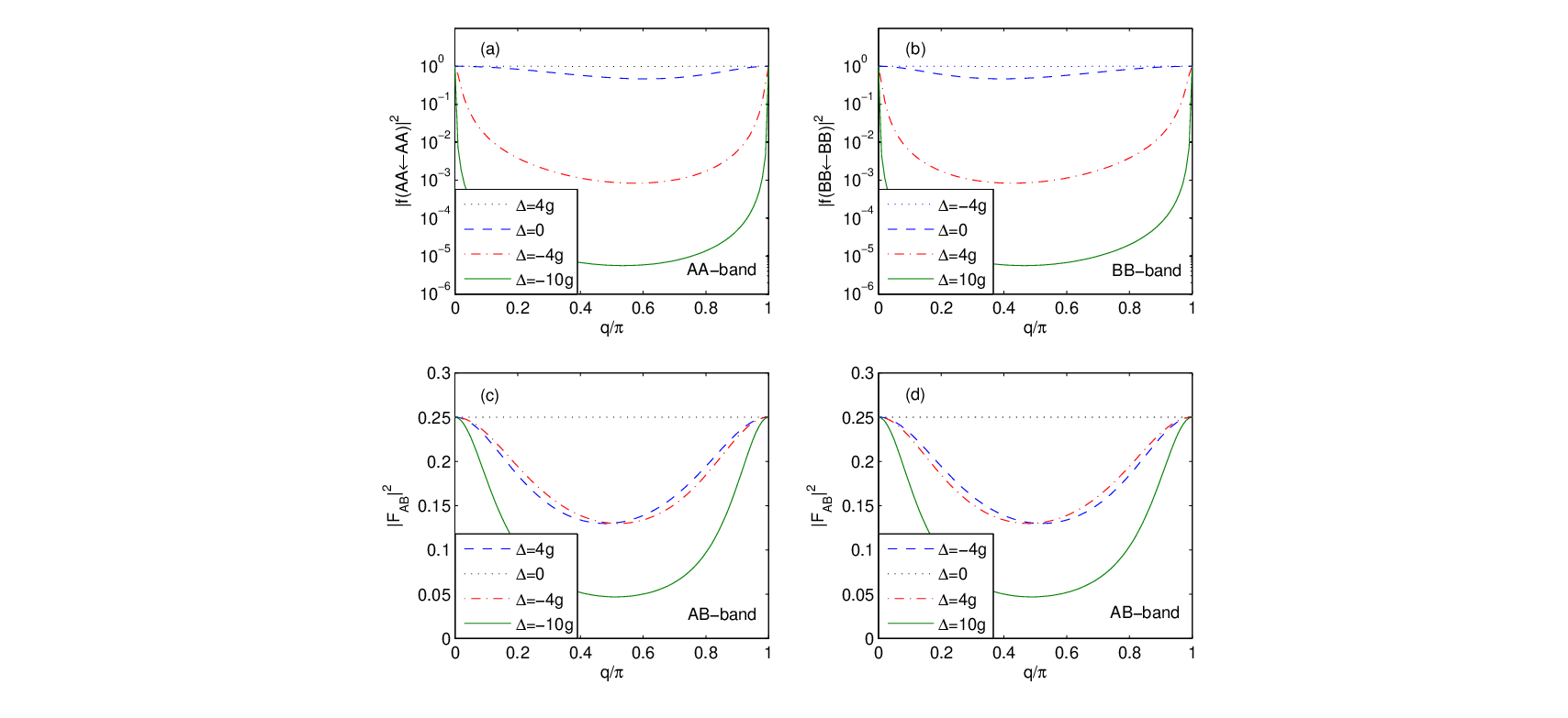
In the 1D low-energy scattering problem of two non-relativistic particles in the continuous space (e.g., the scattering problem of a non-relativistic particle in a delta potential $g\delta(x)$ with $g<0$), it is well-known that, when the energy of the bound state is close to the lower limit of the scattering energies, the scattering coefficient (reflection coefficient) becomes very small. In our system, we find similar resonance results. As shown above, in our cases the band of the scattering energies has both the lower border and the upper border. We find that when the bound-state energy is close to either of these two borders, the relevant scattering coefficient $f$ becomes very small.

For the elastic scattering coefficient $f(AA\leftarrow AA,q)$ of the scattering state in the $AA$ band, as shown in Fig. 3(a), when $\Delta<0$ and $|\Delta|>>|g|,|\xi|$ and $E_{b1}$ is close to the lower bound of $AA$-band, we have $f(AA\leftarrow AA,q)\approx 0$. On the other hand, when $\Delta>>|g|,|\xi|$ and $E_{b1}$ is relatively far from the lower bound of $AA$-band we get the result $|f(AA\leftarrow AA,q)|\approx 1$. Our results show that, the effective interaction between two excitonic polaritons of kind $A$ is negligible in the limit $\Delta\rightarrow-\infty$, and becomes strongly repulsive when $\Delta\rightarrow\infty$.

For the elastic scattering coefficients $f(BB\leftarrow BB,q)$, $f(AB\leftarrow AB,q)$ and the inelastic scattering coefficient $f(BA\leftarrow AB,q)$, as shown in Fig. 3(b), we have $f(BB\leftarrow BB,q)\approx 0$ when $\Delta>>|g|,|\xi|$ and $E_{b2}$ is close to the upper bound of $BB$-band. Finally, for the scattering states in the $AB(BA)$ band, according to our calculation (Fig. 2), the energy $E_{b1}$ is close to the upper bound of the $AB$-band when $\Delta>>|g|,|\xi|$, while $E_{b2}$ is close to the lower bound of the $AB$-band when $\Delta<0$ and $|\Delta|>>|g|,|\xi|$. The corresponding resonance phenomenon is illustrated in Fig. 3(c), where it is shown that in both of these two regions we always have $f(AB\leftarrow AB,q)=f(AB\leftarrow BA,q)\approx 0$.

In this paper we derive the effective interaction between two polaritons in a 1D cavity-array coupled to TLSs, and provide an analytical method for the calculation of scattering and bound states in such a system. We find that in a cavity array there is an effective contact interaction between two polaritons, which is induced by the nonlinearity of the JC Hamiltonian. The interaction is totally determined by the photon-TLS coupling strength $g$, and independent of the photonic hopping intensity $\xi$. For two polaritons with zero center-of-mass momentum, we find that there are two bound states in the gaps between the energy bands of the polaritons, and the 1D resonance phenomenon can appear when the photon-TLS detuning is large enough. Our result is helpful for the research of the few-body and many-body physics of polaritons in cavity arraies. In particular, for the dilute polariton gas where the average polariton number in each cavity is much smaller than one, the many-body physics is dominated by the two-polariton contact interaction.

References

- [1] Lan Zhou, Z. R. Gong, Yu-xi Liu, C. P. Sun, and Franco Nori, Phys. Rev. Lett. 101, 100501 (2008).
- [2] Lan Zhou, Y. B. Gao, Z. Song, and C. P. Sun, Phys. Rev. A 77, 013831 (2008).
- [3] Peng-Bo Li, Ying Gu, Qi-Huang Gong, and Guang-Can Guo, Phys. Rev. A 79, 042339 (2009).
- [4] Shi-Biao Zheng, Chui-Ping Yang, and Franco Nori, Phys. Rev. A 82, 042327 (2010).
- [5] J.-Q. Liao, Z. R. Gong, L. Zhou, Y.-X. Liu, C. P. Sun, and F. Nori, Phys. Rev. A 81, 042304 (2010).
- [6] James Quach, Melissa I. Makin, Chun-Hsu Su, Andrew D. Greentree, and Lloyd C. L. Hollenberg, Phys. Rev. A 80, 063838 (2009).
- [7] M. I. Makin, J. H. Cole, C. D. Hill, A. D. Greentree, and L. C. L. Hollenberg, Phys. Rev. A 80, 043842 (2009).
- [8] M. T. C. Wong and C. K. Law, Phys. Rev. A 83, 055802 (2011).
- [9] D. Rossini and R. Fazio, Phys. Rev. Lett. 99, 186401 (2007).
- [10] D. G. Angelakis, M. F. Santos, and S. Bose, Phys. Rev. A 76, 031805(R) (2007).
- [11] M. J. Hartmann, F. G. S. L. Brandão, and M. B. Plenio, Nat. Phys. 2, 849 (2006).
- [12] M. X. Huo, Ying Li, Z. Song, and C. P. Sun, Phys. Rev. A 77, 022103 (2008).
- [13] A. Mering, M. Fleischhauer, P. A. Ivanov, and K. Singer, Phys. Rev. A 80, 053821 (2009).
- [14] M. J. Hartmann, F. G. S. L. Brandão, and M. B. Plenio, Laser Photonics Rev. 2, 527 (2008).
- [15] M. Aichhorn, M. Hohenadler, C. Tahan, and P. B. Littlewood, Phys. Rev. Lett. 100, 216401 (2008).
- [16] J. Koch and K. Le Hur, Phys. Rev. A 80, 023811 (2009).
- [17] M. I. Makin, J. H. Cole, C. Tahan, L. C. L. Hollenberg, and A. D. Greentree, Phys. Rev. A 77, 053819 (2008).
- [18] S. Schmidt and G. Blatter, Phys. Rev. Lett. 103, 086403 (2009).
- [19] A. D. Greentree, C. Tahan, J. H. Cole, and L. C. L. Hollenberg, Nat. Phys. 2, 856 (2006).
- [20] Ke Liu, Lei Tan, Chun-Hai Lv, and W. M. Liu, Phys. Rev. A 83, 063840 (2011).
- [21] Andrew L. C. Hayward, Andrew M. Martin, and Andrew D. Greentree, Phys. Rev. Lett. 108, 223602 (2012).
- [22] M. Grochol, Phys. Rev. B 79, 205306 (2009).
- [23] An-Chun Ji, X.C.Xie, and W. M. Liu, Phys. Rev. Lett. 99, 183602 (2007).
- [24] K. M. Birnbaum, A. Boca, R. Miller, A. D. Boozer, T. E. Northup and H. J. Kimble, Nature 436, 87 (2005).
- [25] J. R. Taylor, Scattering Theory, Wiley, New York, 1972.