A Quasar-Galaxy Mixing Diagram: Quasar Spectral Energy Distribution Shapes in the Optical to Near-Infrared
Abstract
We define a quasar-galaxy mixing diagram using the slopes of their spectral energy distributions (SEDs) from m to 3000 Å and from m to 3 m in the rest frame. The mixing diagram can easily distinguish among quasar-dominated, galaxy-dominated and reddening-dominated SED shapes. By studying the position of the 413 XMM selected Type 1 AGN in the wide-field “Cosmic Evolution Survey” (COSMOS) in the mixing diagram, we find that a combination of the Elvis et al. (1994, hereafter E94) quasar SED with various contributions from galaxy emission and some dust reddening is remarkably effective in describing the SED shape from m for large ranges of redshift, luminosity, black hole mass and Eddington ratio of type 1 AGN. In particular, the location in the mixing diagram of the highest luminosity AGN is very close (within 1) to that of the E94 SED. The mixing diagram can also be used to estimate the host galaxy fraction and reddening in quasar. We also show examples of some outliers which might be AGN in different evolutionary stages compared to the majority of AGN in the quasar-host galaxy co-evolution cycle.
Keywords:
galaxies: evolution; quasars: general; surveys1 Introduction
The masses of the super massive black holes (SMBHs) that exist in most, if not all, galaxy nuclei (e.g. Kormendy & Richstone 1995), are proportional to their host galaxy bulge stellar mass, as measured by either luminosity (Kormendy & Richstone 1995; Marconi & Hunt 2003) or velocity dispersion (Ferrarese & Merritt 2000; Gebhardt et al. 2000). As most SMBH growth occurs during their active phases (the ‘Soltan argument’, Soltan 1982), most bulges must have gone through an active phase, being seen as a quasar or active galactic nucleus (AGN). It is observed that both galaxies and AGN exhibit coordinated “downsizing”: massive galaxy star formation peaks at , while high luminosity quasars have their peak space density at (Silverman et al. 2005; Brusa et al. 2010; Civano et al. 2011); lower mass galaxies star formation peaks at , as do lower luminosity AGN (Franceschini et al. 1999; Ueda et al. 2003; Brandt & Hasinger 2005; Bongiorno et al. 2007). A close co-evolutionary link between SMBH activity and host galaxy evolution seems to be required.
In principle, we could study whatever feedback process controls this co-evolution, by separately analyzing the emission associated to the SMBH and the host galaxy in the same objects. Observationally, however, it is difficult to disentangle the emission from quasar and host galaxy in the optical-IR range, especially for high redshift () objects. Spatially decomposing a point-source AGN and an extended host requires expensive high-resolution Hubble Space Telescope imaging. Even the 0.1′′ angular resolution of the Hubble cannot easily resolve the extended host emission from the point like AGN emission at (e.g. Cisternas et al. 2011). SED fitting techniques can do so, but have to assume one or several quasar and galaxy SED models (e.g. Merloni et al. 2010), which might lead to systematic errors that are difficult to quantify.
As an alternative approach, we have made use of the fact that the spectral energy distributions (SEDs) of a quasar and of a galaxy near m are completely different. Quasar SEDs show a pronounced dip near m (e.g. Elvis et al. 1994, E94 hereinafter; Richards et al. 2006, R06 hereinafter), while, in contrast, a galaxy SED peaks at around m. This dichotomy allows us to define a diagram of near-infrared (NIR) versus optical (OPT) slopes on either side of m (rest frame) that cleanly separates the two SED forms.
In this diagram (Figure 1), galaxies lie in a well-defined region (, ), that is clearly distinct from the location of the standard AGN SED (, , E94). Reddening moves objects almost perpendicularly to a line joining the galaxy locus to the AGN locus in the diagram. Thus this diagram can distinguish the quasar-dominated, host-dominated or reddening-dominated SEDs easily, without strong model assumptions, and can pick out AGN with mixtures of these three components. Hence we call this the Quasar-Galaxy mixing diagram (hereinafter “mixing diagram” for short).
With this convenient tool, we can more easily study the evolution of quasar SEDs with physical parameters, identify outliers, and estimate host/reddening contributions. This mixing diagram is a generalization of the quasar-galaxy mixing curves in the color-color plane defined for “N galaxies” by Sandage (1971) and Weedman (1973). The plot is equivalent to a color-color plot, but utilizes more photometric bands and is defined in the rest frame. As a result, the mixing diagram can be used for sources at any redshift.
In this paper, we use the mixing diagram to study the the SED shape in the optical to near-infrared decade (m to 3000 Å) for three type 1 AGN samples: the large XMM-COSMOS type 1 AGN sample (Elvis et al. 2012, Paper I hereinafter), the SDSS-Spitzer quasar sample (R06) and the bright quasar sample (E94). Detailed description of the three samples are in § 3.1. We primarily focus on the XMM-COSMOS type 1 AGN sample to demonstrate the major applications of the mixing diagram.
All the wavelengths considered in this paper are in the rest frame. We adopt the WMAP 5-year cosmology (Komatsu et al. 2009), with , and .
2 Quasar-Galaxy Mixing Diagram
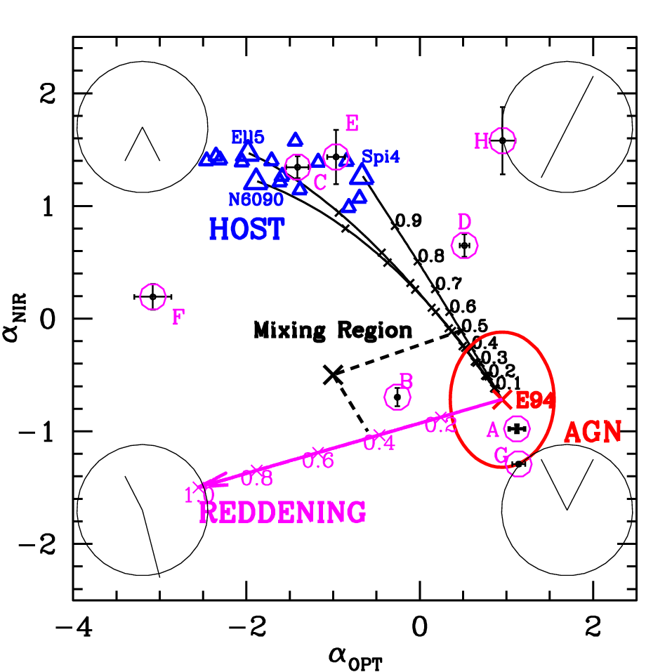

The mixing diagram axes are the m (rest-frame) SED power-law slope () versus the m (rest-frame) power-law slope (), where . These ranges lie on either side of the m dip, or inflection point, of the rest frame SED.
The m wavelength point is not chosen as the central point arbitrarily. This is where the Wien tail of the black body thermal emission of the hottest dust (at the maximum sublimation temperature of , Barvainis et al. 1987) begins to outshine the optical band power-law ( -0.3) of the SMBH accretion disk (Malkan & Sargent 1982; Sanders et al. 1989; E94; Glikman et al. 2006).
We tried several different wavelength ranges to calculate the slopes and found that the adopted ranges best represent the dip around m. If a smaller wavelength range is chosen, the number of photometric points in the range will be greatly reduced, due to the relatively limited photometry coverage (only J H K band) in the NIR range. If a longer wavelength range is chosen, a variety of problems would make the estimates of the slope more difficult. For example, shorter wavelengths, into the UV, are more affected by variability and by the FeII ‘small bump’ (Wills, Netzer & Wills, 1985); longer wavelengths in the NIR encounter a range of cooler dust emission which adds noise to the NIR slope. In the chosen wavelength range, the XMM-COSMOS type 1 AGN SED dispersion is invariant in a large range of and (Hao et al. 2013a, Paper II hereinafter), which implies an invariant intrinsic dispersion of SED shape in this wavelength range.
To ensure reliable slopes, we require at least 3 photometric points to define each slope. The robustness of the slope measurement using 3 or more photometric points was tested in Hao et al. (2011) and found to be good. For the XMM-COSMOS quasar sample, the optical data set is so rich that the mean number of photometry points used in calculating is 11.46.1, while the infrared data is less rich and the mean number of photometry points used in calculating is 4.30.7. The errors on the slopes ( and ) are the standard errors of the linear fit. The measurement error on the photometry is used in the fitting.
The major characteristics of the mixing diagram are shown in Figure 1. The E94 radio-quiet (RQ) mean SED template is shown by a red cross. This template is bluer than almost all COSMOS XMM quasars (Paper I), probably due to the selection criterion used to select it (Schmidt & Green 1983). The 16 galaxy templates11 1 The 16 galaxy templates in the “SWIRE Template Library” (Polletta et al. 2007) include: 3 elliptical galaxy templates “Ell2”, “Ell5”, “Ell13” representing elliptical galaxy of age 2 Gyr, 5 Gyr and 13 Gyr respectively; 7 spiral galaxy templates “S0”, “Sa”, “Sb”, “Sc”, “Sd”, “Sdm”, “Spi4”; and 6 starburst galaxy templates “NGC6090”, “M82”, “Arp220”, “IRAS20551-4250”, “IRAS22491-1808”, “NGC6240”. from the “SWIRE Template Library” (Polletta et al. 2007) are shown as blue triangles in the left panel of Figure 1. Lines joining the E94 mean SED to three representative galaxy templates are drawn. These mixing curves are marked at 10% intervals of host galaxy contribution (see § 2.3 for details).
Note that the slopes are defined in versus plane. Different SED shapes lie in different regions of the mixing diagram, as sketched inside the circles in the four corners of the left panel (wavelength increases to the left in these circles): the bottom right corner shows the m inflection of an AGN dominated SED; the upper left corner shows the cool starlight peak of a galaxy dominated SED; the bottom left corner shows the rapid drop in the optical characteristics of a dust reddening dominated SED. The top right corner shows an SED falling throughout the entire optical-NIR range. This was not a known SED shape until the recent discovery of “hot dust poor” AGN (HDP hereinafter, Jiang et al. 2010; Hao et al. 2010, 2011), which make up 10% of the quasar population (Hao et al. 2011).
We will discuss in detail the major characteristics of the mixing diagram as shown in the right panel of Figure 1 in the following sub-sections.
2.1 Quasar Templates
Besides the E94 quasar SED template, there are several recent updates (R06; Hopkins et al. 2007; Shang et al. 2011; Paper I). The comparison of these SED templates were discussed in Paper I.
The R06 SED template was compiled from the Spitzer-SDSS sample, containing 259 AGN and used a “gap repair” technique that replaces the missing photometry with the normalized E94 mean SED to the adjacent available photometry bands. Due to the limited coverage in near-infrared, the R06 mean SED is therefore, by construction, very similar to the E94 mean SED. Hopkins et al. (2007) simply combined the R06 mean SED with the composite quasar SED (Vanden Berk et al. 2001), thus it has a shape similar to both R06 and E94. As we can see in the right panel of Figure 1, the R06 ( and ) represented with a pentagon and the Hopkins et al. (2007) template ( and ) represented with a hexagon are very close to the E94 template ( and ) represented with a cross.
The Shang et al. (2011) mean SED ( and ) was calculated using 27 nearby bright radio-quiet quasars. As there is limited coverage in infrared (only 3 points in the near-infrared range from the template), there is a large error bar in the near-infrared slope calculation. The Shang et al. (2011) template is represented with a triangle in the right panel of Figure 1.
Paper I studied 413 XMM selected COSMOS type 1 AGN. Due to the X-ray selection, there are more quasars in this sample having a large host contribution (see also § 3.2). 203 quasars in the sample can be corrected for host galaxy contribution from the Marconi & Hunt (2003) scaling relationship adding an evolutionary term (Bennert et al. 2010, 2011). The mean host-corrected SED of the 203 XMM-COSMOS quasars is represented with a square in the right panel of Figure 1. We can see that there is still an indication of a excess of host contribution, that remains un-corrected. This is likely due to the dispersion in the scaling relationship.
Given the similar location of these templates in the mixing diagram, the results derived from the mixing diagram (e.g., host galaxy fraction, reddening etc) would not be significantly affected if R06 or Hopkins et al. (2007) templates are chosen instead of E94. Shang et al. (2011) and Paper I have other contamination factors in the templates themselves that render them not proper to be chosen as the pure quasar template. So we will use E94 template to represent pure quasar SED template for future discussion in this paper.
2.2 Galaxy Templates
The 16 SWIRE galaxy SED templates are all from the observations of various types of galaxies (Polletta et al. 2007). Theoretically, models of the galaxy SEDs have been developed based on the stellar population synthesis technique (Bruzual & Charlot 2003, BC03 hereinafter). These models have been successfully used in SED fitting especially in the optical range (e.g., Ilbert et al. 2009; Ilbert et al. 2010; Bongiorno et al. 2012). However, these models do not include the dust attenuation and re-radiation, and we are still not sure if all the SEDs produced from these models exist in real universe. Here we plot (Figure 1, right) the BC03 SED models on the mixing diagram in comparison with the Polletta et al. (2007) observed galaxy templates.
In the right panel of Figure 1, the galaxy SED model is computed using the preferred Padova 1994 evolutionary tracks (Alongi et al. 1993; Bressan et al. 1993; Fagotto et al. 1994 a, b; Girardi et al. 1996) assuming a universal initial mass function (IMF) from Chabrier (2003) and an exponentially declining star formation history. The star formation rate is expressed as , where is the e-folding timescale. We show models for 16 different e-folding timescales Gyr, ranging a variety of star-formation history.
The lines shown are for galaxies with ages () running from 0.1 Myr to 20 Gyr for each e-folding timescale model. The black tick points on the lines are for a galaxy model with Gyr in steps of . For different e-folding timescales, the young galaxies ( Gyr) are quite similar to each other. However, for older galaxies ( Gyr), the positions in this plot are quite different for different e-folding timescales. For example, for Gyr model (blue solid line), the oldest galaxy ( Gyr) reaches the leftmost region of the diagram and for Gyr model (red solid line), the oldest galaxy ( Gyr) only reaches the Spi4 position. All the galaxies in the Gyr model fail to overlap with the observed Polletta et al. (2007) galaxy region. When we increase the e-folding timescale, the position of the galaxies with the same age at Gyr move from the left to the right on the diagram. The distances among the lines on the mixing diagram with different e-folding timescales lie within the error bar of the slopes except for the Gyr model, which show a wave at . This wave also exists in other lines with smaller size and at . The wave may caused by the molecular feature in the atmosphere of cool/old stars.
From Gyr, the values are almost constant compared to the huge change in . This is reasonable because the near-infrared SED mainly comes from the emission of old stars whereas the optical SED mainly comes from the emission of young stars. As an exponentially declining star formation history is assumed, when the galaxy gets old enough, the star-formation rate is low, which means the young star population becomes very small. So the optical SED changes a lot, but the near-infrared SED almost stays constant.
| Spi4 | Ell5 | Sb | S0 | NGC6090 | ||||||
|---|---|---|---|---|---|---|---|---|---|---|
| 0.0 | 0.950 | -0.719 | 0.950 | -0.719 | 0.950 | -0.719 | 0.950 | -0.719 | 0.950 | -0.719 |
| 0.1 | 0.876 | -0.621 | 0.857 | -0.618 | 0.862 | -0.617 | 0.860 | -0.617 | 0.864 | -0.620 |
| 0.2 | 0.794 | -0.513 | 0.752 | -0.506 | 0.762 | -0.506 | 0.759 | -0.506 | 0.766 | -0.511 |
| 0.3 | 0.702 | -0.394 | 0.634 | -0.382 | 0.648 | -0.383 | 0.641 | -0.383 | 0.655 | -0.392 |
| 0.4 | 0.598 | -0.262 | 0.496 | -0.244 | 0.515 | -0.246 | 0.505 | -0.245 | 0.525 | -0.260 |
| 0.5 | 0.480 | -0.112 | 0.334 | -0.086 | 0.357 | -0.090 | 0.341 | -0.089 | 0.372 | -0.111 |
| 0.6 | 0.342 | 0.060 | 0.138 | 0.097 | 0.164 | 0.089 | 0.140 | 0.091 | 0.184 | 0.059 |
| 0.7 | 0.178 | 0.263 | -0.109 | 0.316 | -0.082 | 0.302 | -0.119 | 0.304 | -0.053 | 0.257 |
| 0.8 | -0.024 | 0.509 | -0.439 | 0.586 | -0.415 | 0.563 | -0.475 | 0.566 | -0.373 | 0.497 |
| 0.9 | -0.286 | 0.823 | -0.934 | 0.941 | -0.925 | 0.902 | -1.037 | 0.906 | -0.857 | 0.800 |
| 1.0 | -0.656 | 1.264 | -1.972 | 1.469 | -2.044 | 1.396 | -2.447 | 1.403 | -1.876 | 1.218 |
1 A portion of the table is shown here for guidance. The complete table for 16 SWIRE galaxy templates will be available online.
Compared to SWIRE galaxy templates, the BC03 models show very blue galaxies located on the upper right corner of the mixing diagram and show less spread in the direction. The blue galaxies are typically very young and they would be expected to contain large amount of gas. These galaxies are very rare in the redshift range of current major surveys and tend to be more common for high reshifts (, Bouwens et al. 2012). These very blue galaxies are so extremely short-lived that they are expected to be a very small fraction in any sample of galaxies. For example, in Ilbert et al. (2010), SED fitting analysis is performed to IRAC selected galaxies with in the COSMOS field. They find that only a few percent have Gyr and most of them are fitted with a significant extinction.
One would suspect that the presence of a young population on top of an older population could mimic a blue non-thermal quasar-like optical spectrum. However, in practice, the chance is low, because, to reach the slope, the star-formation rate of the young population would be too extreme. Also, if this were commonly true, optically selected type 1 AGN would be severely diluted by starbursts, which is not seen.
The possible presence of very young galaxy models also provides an alternative explanation to the HDP AGN SED that is the normal quasar SED with large fraction of young host galaxy. But this explanation would require the quasar to be active simultaneously with a strong starburst, which is not seen in large samples (e.g. Kewley et al. 2006, Schawinski et al. 2009, Wild et al. 2010).
In this paper, to be consistent with the quasar template we use (E94, which has been derived from observed SEDs), we only use the observed Polletta et al. (2007) SWIRE galaxy templates for further discussion.
2.3 Galaxy Fraction Mixing Curves
We can quantify the host galaxy contribution fraction at m for any quasar, assuming that the E94 RQ template represents a pure AGN SED. A definition similar to is widely used in SED fitting with different normalization wavelengths (e.g. Salvato et al. 2009, Merloni et al. 2010). The parameter is defined as the galaxy fraction at m, and describes how close the observed SED is to the galaxy templates. First, we normalize both the galaxy and AGN template at m. Then the mixture of some fraction of galaxy () and some fraction of AGN (1-) emission can be calculated accordingly. Suppose that at frequency the galaxy template SED luminosity is and the AGN template (E94) SED luminosity is , then the mixing of the two SEDs luminosity is
The black curves in Figure 1 show the slopes of SED templates obtained by mixing the AGN and galaxy templates with values of . The mixing curves of the starburst galaxy “NGC6090” and the spiral galaxy “Spi4” define the red and blue boundaries of the possible slopes obtained by mixing the E94 SED with all 16 galaxy templates in the SWIRE library. The spectral slopes for mixtures of E94 with Spi4, Ell5, Sb, S0, and NGC6090 for 11 values of are listed in Table 1. The complete table for all the 16 templates is available on line.
2.4 Reddening Vectors
| Ext. Law | SMC | LMC | MW | Calz | ||||
|---|---|---|---|---|---|---|---|---|
| 0.0 | 0.950 | -0.719 | 0.950 | -0.719 | 0.950 | -0.719 | 0.950 | -0.719 |
| 0.1 | 0.596 | -0.798 | 0.596 | -0.798 | 0.604 | -0.807 | 0.553 | -0.890 |
| 0.2 | 0.242 | -0.877 | 0.242 | -0.877 | 0.257 | -0.895 | 0.156 | -1.060 |
| 0.3 | -0.112 | -0.956 | -0.112 | -0.956 | -0.089 | -0.982 | -0.241 | -1.231 |
| 0.4 | -0.465 | -1.034 | -0.465 | -1.034 | -0.435 | -1.070 | -0.639 | -1.402 |
| 0.5 | -0.819 | -1.113 | -0.819 | -1.113 | -0.781 | -1.158 | -1.036 | -1.572 |
| 0.6 | -1.173 | -1.192 | -1.173 | -1.192 | -1.128 | -1.246 | -1.433 | -1.743 |
| 0.7 | -1.527 | -1.271 | -1.527 | -1.271 | -1.474 | -1.333 | -1.830 | -1.914 |
| 0.8 | -1.881 | -1.350 | -1.881 | -1.350 | -1.820 | -1.421 | -2.227 | -2.084 |
| 0.9 | -2.235 | -1.428 | -2.235 | -1.428 | -2.166 | -1.509 | -2.624 | -2.255 |
| 1.0 | -2.588 | -1.507 | -2.588 | -1.507 | -2.513 | -1.597 | -3.021 | -2.426 |
Intrinsic reddening in AGN is often important in defining their SEDs (e.g., Ward et al. 1987; O’Brien et al. 1988; Young et al. 2008; Shang et al. 2011). The magenta arrows in Figure 1 show and for the E94 SED when reddened by .
We consider four different reddening laws: Small Magellanic Cloud (SMC), Large MC (LMC), Milky Way (MW), and Calzetti et al. (2000, Calz). For the SMC, LMC, and MW reddening laws, the reddening of the E94 SED is derived with the IDL de-reddening routines ‘FM_UNRED.PRO’(for SMC and LMC) and ‘CCM_UNRED.PRO’ (for MW), which all use the Fitzpatrick (1999) parameterizations of the SMC (Gordon et al. 2003), LMC (Misselt et al. 1999), and the MW (Cardelli et al. 1989; O’Donnell 1994) extinction curves. For the Calz reddening law, the reddening is derived with IDL de-reddening routine ‘CALZ_UNRED.PRO’, which uses the Calzetti et al. (2000) recipe developed for galaxies where massive stars dominate the radiation output. The SMC reddening law (Gordon et al. 2003) is typically used for quasars, and is shown to fit reddening in quasars more effectively than a LMC or MW reddening law (Hopkins et al. 2004; Richards et al. 2003). Reddening primarily affects . The effect of reddening is reported in Table 2.
Using the reddening vector, we can estimate and from the mixing diagram for sources lying off the E94-host mixing curves toward the lower left. For each source we can draw a line parallel to the reddening curve (black dashed line in Figure 1). The crossing point of this line and the mixing curve shows approximately the value of . The length of the parallel line gives an estimate of . We use this technique in § 4.2 and § 4.3.
Different reddening laws could cause different and derived from the mixing diagram. As we can see from the right panel of Figure 1, the SMC, LMC, and MW reddening vectors are closely similar to each other. The Calz reddening vector is significantly different from the other three reddening laws. This reddening law is generally used for star-forming galaxies (Calzetti et al. 2000) not AGN. Gordon et al. (2003) performed a comparison between SMC, LMC, and MW reddening laws and found that the extinction curves only begin to diverge shortward of Å and at rest frame near-UV (Å) through near infrared (m), the three laws are extremely similar. So for the rest frame wavelength range in which the mixing diagram is defined (3000Å to m and m to m), the results will not be significantly different if we choose either SMC, LMC or MW reddening law. We will only consider the SMC reddening law in the following discussion.
3 Mixing Diagram for Type 1 AGN Samples
3.1 Type 1 AGN Samples


The three type 1 AGN samples we used in this paper are:
(1) The XMM-COSMOS type 1 AGN Sample (XC413, Paper I). The COSMOS field (Scoville et al. 2007) was imaged in X-rays with XMM-Newton for a total of Ms (Hasinger et al. 2007; Cappelluti et al. 2007, 2009). Optical identifications were made by Brusa et al. (2007, 2010) for the entire XMM-COSMOS sample, who gave photometric properties and redshifts for each X-ray point source. From this complete sample, we extracted a sample of 413 type 1 AGN, defined by having broad line FWHM2000 km s-1. The XC413 catalog was described in detail in Paper I.
This sample has full wavelength coverage from radio to X-ray (for a total of 43 photometric bands, Paper I) and high confidence level spectroscopic redshifts (Trump et al. 2009; Schneider et al. 2007; Lilly et al. 2007, 2009). In this paper, we also add the recently released H band photometry from CFHT/WIRCAM (McCracken et al. 2010). Now 405 out of the 413 XMM-COSMOS quasars have H band photometry, compared to 252 out of 413 in Paper I. As described in Paper I, the photometric data obtained from different telescopes and with different seeing were matched and the aperture fluxes were all transformed to total flux according to the point spread function simulation for each telescope (e.g., Capak et al. 2007, Brusa et al. 2007). As in Paper I, in order to reduce the extra error in the SED slope measurement that can be caused by variability of quasars, we used only the optical photometric data obtained in a shorter time period (2004-2008) close to the time of the infrared Spitzer-IRAC data. The COSMOS type 1 AGN sample has an extremely rich coverage (36 bands) in the optical to near-infrared range. The objects have redshifts and magnitudes , with 94% - 98% being radio-quiet (Hao et al. 2013b).
In this sample, 206 quasars have published black hole mass measurements (Trump et al. 2009b; Merloni et al. 2010), which are based on the scaling relationship between broad emission line (BEL) FWHM and black hole mass (Vestergaard 2004). For the quasars with only zCOSMOS spectrum, the black hole mass was estimated for only those with MgII lines in the spectrum (Merloni et al. 2010), using the calibration of McLure & Jarvis (2002). For the rest of the sample, the BELs are located close to the ends of the spectra, so reliable black hole mass estimates cannot be made. We call the sub-sample with black hole mass estimates SS206 (‘SS’ stands for sub-sample) hereinafter.
(2) The SDSS-Spitzer Sample (R06). The R06 sample consists of 259 Spitzer sources identified with Sloan Digital Sky Survey (SDSS) quasars in four different degree-scale fields, and is, therefore, mid-IR identified and optically selected. The redshift range covered is with 93% being at . Most (215/259) of the R06 sources did not have 2MASS J H K photometry. Details about how we measured the slopes with this sample were described in Hao et al. (2011).
(3) The bright quasar sample (E94). This sample consists of 42 quasars in the redshift range , with 80% of them being at . The optical photometry was obtained at the FLWO (F. L. Whipple Observatory) 24 inch telescope within one week of the MMT FOGS (Faint Object Grism Spectrograph) spectroscopic observations. The NIR data were obtained with MMT and IRTF. More details on the observation can be found in E94. The E94 SEDs have been corrected for host galaxy contamination by subtracting the host galaxy template SED based on the Sbc galaxy model of Coleman et al. (1980). The E94 sample has bolometric luminosities (log) in the range of erg/s with mean of 45.75 erg/s. We recalculated the E94 bolometric luminosities with the same cosmological parameters used for XC413. Compared to XC413, E94 sample is on average more luminous and contains less low luminosity quasars than the XC413. The Eddington ratio of the PG quasars (including E94 sample) is comparable to that of the XC413 (Sikora et al. 2007, Paper II).
3.2 Mixing Diagram for the Quasar Samples
We plot the XC413 sample on the mixing diagram in Figure 2. The distribution is continuous and largely lies between the E94 mean SED and the galaxy templates, along the mixing curves, with some spread in the reddening direction to values as large as , but mostly with . The green crosses represent objects with black hole mass estimates (Paper II), which span the range of the entire sample in the mixing diagram.
The diagram shows that about 90% of the sources lie in the left hand triangular ‘mixing wedge’ between the mixing curves and the reddening vector. The SEDs of these AGN can be accounted for with a simple combination of an E94 quasar SED, plus a galaxy contribution and reddening. This suggests that the AGN sample is consistent with a single intrinsic SED shape, closely resembling the E94 mean quasar SED (see also in § 4.1, where we compare in detail the XC413 and the E94 quasar sample).
There are several sources outside the wedge, which are outliers with respect to the bulk of the type 1 AGN population (see § 4.4 for details). As the galaxy SED dispersion is expected to be broader than the 16 Polletta templates, it is not surprising to see three sources (XID=4, 1559, 5617) beyond the SWIRE galaxy template region (still within 1) that would formally require . We excluded these sources when using the mixing diagram to calculate (see § 4.2 for details).
We also plot the mixing diagram for the SDSS-spitzer quasar sample (R06) and the bright quasar sample (E94), shown in Figure 3 (see also Hao et al. 2011). For the optically-selected R06 sample, quasars by selection are more clustered in the quasar dominated region unlike the X-ray-selected XC413, which includes more sources with low quasar to host galaxy contrast. The E94 quasars have been corrected for host galaxy contribution. Thus they are, by construction, clustered around the E94 mean (red cross) in the quasar dominated region. Compared to the E94 sample, the R06 sample is not as blue in the optical.
3.3 Intrinsic Slope Dispersion


We selected a sub-sample of AGN-dominated XC413 SEDs with in order to exclude galaxy- or reddening-dominated sources. This sample has a mean slope =0.63 (standard deviation =0.24), and (standard deviation =0.36). The E94 RQ mean ((E94) = 0.95, (E94), see values in Table 1 for =0) lies at the extreme blue end of the distribution.
To estimate the intrinsic dispersion within the AGN-dominated XC413 sub-sample we removed the effect of measurement error, namely: . The mean of the measurement error for is = 0.09, and for is = 0.12. The intrinsic dispersion thus is = 0.22 and = 0.34 respectively. Therefore, the intrinsic dispersion of the SED shape is 2 - 3 times the measurement error and seems to be significant.
The equivalent intrinsic dispersions in the E94 and R06 sample were estimated by Hao et al. (2011), who found: = 0.25, = 0.32, = 0.23, and = 0.36, respectively. The intrinsic dispersions are thus similar for all the three samples.
To compare the intrinsic dispersion of these three samples more rigorously, we applied the Bayesian method of Kelly et al. (2007). This assumes that the intrinsic distribution of the slopes is a mixture of Gaussians. The probability distributions of the differences in slope dispersion between the samples are shown in Figure 4. For the dispersion in , the significance of the difference between the XMM-COSMOS and R06 sample is 0.16; between XMM-COSMOS and E94 sample is 0.11 and between R06 and E94 sample is 0.08. Therefore, the intrinsic dispersions of the are consistent with being the same for all the three samples. For , the significance of the difference between the XMM-COSMOS and R06 sample is 0.02; between the XMM-COSMOS and E94 sample is 0.08 and between the R06 and E94 sample is 0.06. As in the simpler analysis, the intrinsic dispersions of the and are consistent with being the same for all the three samples.
Using this result we can create a more rigorous AGN-dominated sample using the intrinsic dispersion to define a radius in the (, ) plane within which such AGN must lie. As the distribution of the quasars is continuous, different radii define different populations of quasars. We define a circle centered on the E94 RQ mean SED template with a radius of 0.6 on the mixing diagram to define AGN-dominated sources. This is approximately 3 and 1.5 of the intrinsic dispersion. Note that the AGN dominated circle chosen here is somewhat arbitrary and is used just for illustration. Different radii or even shapes of the AGN-dominated region can be chosen for different purposes. For the XC413 sample, the sources within the dispersion circle populate mainly the left upper quadrant, similar to the R06 sample, but unlike the host-corrected E94 sample. We will discuss this more in section § 4.1.
4 Application of the Mixing Diagram to the XC413 Sample
4.1 SED Evolution on the Mixing Diagram


Paper II studied the evolution of the mean and dispersion of the SED with physical parameters (redshift , bolometric luminosity , black hole mass , and Eddington ratio 22 2 ) for the 407 radio quiet quasar in the XC413 sample. Paper II showed that there is no obvious evidence for evolution of the quasar SED shape with respect to these parameters. The study was limited by the difficulties of host galaxy subtraction. The conclusions are fully based on the assumption that host galaxy correction according to the black hole mass and bulge mass scaling relationship adding an evolutionary term is reliable. The mixing diagram is a new tool to address this issue, with no need to rely on the assumption that the host correction is properly done. That is because the diagram itself can clearly show the contribution from the host galaxy.
In order to search for quasar SED evolution with respect to physical parameters, we plotted the mixing diagram for the XC413 sample in bins of , , and for the SS206 sample with two additional parameters and , because the black hole mass estimates are only available for these 206 quasars in XC413 (see § 3.1). We divided the sample in four bins: in [0 – 1 – 2 – 3 – 4.3], in [44.2 – 45.2 – 45.8 – 46.4 – 47.3], in [7.1–7.7–8.3–8.9–9.4], and in [-1.9 – -1.2 – -0.6 – 0 – 0.7], respectively. For each physical parameter the four bins have approximately equal bin size, so it is easy to compare bins. The resulting mixing diagrams are shown in Figures 5 and Figure 6.
To look for any SED evolution in smaller steps, we color coded the quasars in each bin for four equal sub-bins (Figure 5 and Figure 6). In each and mixing diagram, the black, red, green, and blue points represent quasars with small to large and , with the sub-bin size of 0.25. Similarly, in each and mixing diagram, the black, red, green and blue colors represent small to large values, with sub-bin size of 0.15.
For the lowest bin of each parameter (, , , ), almost all of the sources lie within the mixing wedge defined by the AGN-host mixing curve, allowing for the range of the E94 mean SED slope, mixing curve and the reddening curve.
For high values of each parameter, the quasars (Figure 5 and Figure 6) cluster close to the quasar dominated region (within the red circle), while in the lower value bins the quasars spread out along the mixing curves toward the galaxy template locations. This effect is the strongest in bins. For different bins, the cluster of quasar locations clearly drifts along the mixing curves, from completely outside the AGN-dominated circle at low , with many sources lying near the pure galaxy-dominated region, to almost completely inside the dispersion circle at high . This is expected, as the galaxy luminosity is generally no more than erg/s (Cirasuolo et al. 2007). Thus for extremely high luminosity sources, the AGN outshines the galaxy, especially in the optical. However, the M- relation puts a limit on how much a quasar can outshine its host galaxy (Paper I, II).
Although almost all of the highest luminosity quasars (Figure 5) lie within the AGN-dominated circle, they are not centered at the E94 RQ mean. Instead they lie overwhelmingly in the upper left quadrant of the dispersion circle, similar to the R06 sample as shown in the left panel of Figure 3. This suggests that some shift with respect to the E94 SED is present in both spectral slopes. For these highest luminosity quasars, the mean is 0.78, versus 0.95 for E94 mean SED, with ; and the mean is -0.44, versus -0.72 for E94 mean SED, with . In XC413 the slopes of the highest luminosity quasars are shifted by 1 relative to the E94 RQ mean SED. This may be an intrinsic shift, or may indicate a non-negligible host galaxy component even in these luminous quasars.
To compare in detail the highest luminosity quasars in XC413 and E94, we checked the 8 E94 quasars which lie in the same highest luminosity range (above erg/s). The mean of these 8 high luminosity E94 quasars is 0.93 with , almost exactly the same as the optical slope of E94 mean SED, and bluer () than the XC413 high luminosity quasars. Instead, the mean of these 8 E94 quasars is -0.19, with , which is much flatter than the NIR slope of E94 mean SED, and even flatter than the XC413 high luminosity quasars. This difference is mainly due to the two hot-dust-poor quasars in these 8 E94 quasars (Hao et al. 2011). From this comparison, we can only conclude that the highest luminosity E94 quasars are bluer than the highest luminosity XC413 quasars. We are not sure if this result can be explained by selection effects only.
In the higher bins, a population of outliers is present toward the top right corner. These outliers are the hot-dust-poor (HDP) quasars discussed in detail in Hao et al. (2010, 2011). The fraction of sources outside the mixing wedge is quite similar in the top three , and bins. This result agrees with the lack of evolution in HDP fraction with and (Hao et al. 2010, 2011).
In first approximation, the contrast between nuclear AGN continuum and host galaxy in B band (rest-frame) can be expressed in a single formula (Merloni & Heinz 2012):
where is the mass-to-light ratio of the host galaxy and (B/T) is the bulge-to-total galactic stellar mass ratio. So for typical mass-to-light ratios and bulge-to-total galactic stellar mass ratios, the contrast will be smaller if is smaller, hinted as shown in the bottom row of Figure 6, from left to right. When is getting larger, the quasars generally drift towards the quasar dominated direction (smaller ).
A minority of XC413 quasars in each of the lower bins of , lie in the highly reddened region (, Figure 5). For example, for the lowest bin, the fraction is 6% (4 out of the 71 sources). In SS206 (Figure 6), quasars in the highly reddened region only exist in the lower bins of and . This effect is not so evident in and , where a small fraction of highly reddened quasars appear in high or bins. Extremely low Eddington ratio AGN () tend to have red optical SED, unlike the typical quasars () with “big-blue-bump” (Ho et al. 2008, Trump et al. 2011). In SS206, we do not see any obvious trend that small Eddington ratio quasars are more reddened for the typical quasars. This is probably due to the small Eddington ratio range in SS206 compared to the large difference between the low luminosity AGN and the normal AGN.
4.2 Inferred Host Galaxy Fraction


The mixing diagram provides a new estimate of the galaxy fraction (§ 2.4). The errors on the estimates are caused by the error on the slopes, due to linear fitting of the SEDs. Different galaxy templates also give slightly different values. Figure 7 compares the values for two templates. The differences are negligible and almost unbiased, compared to the errors on . The correlation coefficient is 1 (precise to the 4th place after decimal). If we fit a straight line, the best fit slope is , very close to 1.
We can compare with host galaxy fractions derived with three other methods: using bulge - black hole scaling relations, direct imaging and SED fitting. The three methods are briefly described below:
(1) Black hole mass - Galaxy bulge scaling relations: For the 203 quasars in SS206, following Paper I, we used the relationship between the black hole mass and near-infrared bulge luminosity (Table 2 of Marconi & Hunt, 2003) adding an evolutionary term (Bennert et al. 2010, 2011) to estimate the host galaxy contribution:
| (1) | |||||
We used the Ell5 galaxy template to calculate the rest frame m host luminosity. In this band the differences among different galaxy templates are small. With the host luminosity we can calculate the galaxy fraction at rest frame m (). The rest frame J band (m) luminosity is used because this is the band closest to m, and is where the galaxy contribution peaks.
The small photometric errors in J imply that black hole mass measurement errors dominate the error on . Black hole mass estimates from mass scaling relationships have an error (Vestergaard & Peterson 2006; Peterson 2010), so , as (according to Equation 1).
(2) Direct imaging: For 94 low redshift () quasars in the XMM-COSMOS sample, Cisternas et al. (2011) used the Hubble images to decompose the AGN and galaxy emission and to estimate the host galaxy fraction at 8140Å (observed frame). We transformed this galaxy fraction to the rest frame m galaxy fraction () using the Ell5 galaxy template. As only the best fit model of the host galaxy luminosity is given, we cannot estimate the error on due to the fitting process.
However, the assumed template introduces an uncertainty. The observed F814W photometry point lies on the steep side of the galaxy template for . Hence, a small error in template slope (or, effectively, in the age of the youngest stellar population in the host) would lead to a large error in the host estimate at m. We can use this extrapolation uncertainty to estimate a minimum error. To do so, we normalized the 16 SWIRE galaxy templates (Polletta et al. 2007) at m and measured the dispersion of these different templates at the rest frame wavelength corresponding to the observed 8140Å. We use these dispersions as errors on the host galaxy luminosities at m for sources at different redshifts. Therefore, the error on the galaxy fraction can be estimated as . The error bar ranges from 0.02 to 0.77 with the median value of 0.21.
(3) With the multi-wavelength photometry data available, SED fitting can be used to decompose the observed SEDs with some assumptions on the intrinsic component SEDs. Bongiorno et al. (2012) used R06 with SMC like dust-reddening (Prevot et al. 1984), and BC03 models with Calzetti reddening (Calzetti et al. 2000) to fit the XMM-COSMOS sources. We calculate the galaxy fraction and host galaxy luminosity at rest-frame m from their SED fitting and compare them with the results derived directly from the mixing diagram.
The comparison of estimated from the mixing diagram with the galaxy fraction from the other three methods (from Paper I), (from Cisternas et al. 2011) and (from Bongiorno et al. 2012) is shown in the top row of Figure 8. For ease of comparison, we also plot the ratio of the values from the other three methods over from the mixing diagram versus the from mixing diagrm in the second row.
The first two methods (scaling relationships and direct imaging decomposition) give values which are poorly correlated with the values from the mixing diagram. The correlation coefficient for and is 0.35, for and is -0.09. gives systematically smaller values than the other methods. From equation 1, this effect is either due to a systematic underestimate of black hole mass, or to an over-estimate of the evolution of the scaling relationship, which may be more likely (see e.g., Schramm & Silverman 2013).
However, the values from the SED fitting are strongly correlated with the values from the mixing diagram, although with a shift in normalization. The correlation coefficient between the two sets of values is 0.83. The host galaxy fraction from the SED fitting is systematically slightly higher than the results of the mixing diagram. This is probably due to the galaxy template model employed. The SED fitting in Bongiorno et al. (2012) used BC03 models, which generally have smaller so the mixing curves are shorter, leading to larger galaxy fractions (see right panel of Figure 1).
The inferred m host galaxy luminosities (, , and ) are also compared in Figure 8 (bottom two rows). The correlation coefficient between and is 0.17, between and is 0.33 while that between and is 0.75. For most cases the inferred host galaxy luminosity is less than erg/s (that is ), a reasonable value, as at (Cirasuolo et al. 2007).
Using the mixing diagram to estimate the host galaxy fraction requires the following assumptions: 1) an intrinsic quasar SED exists and is similar to E94 mean SED; 2)the chosen galaxy templates are representative; 3) all the quasars have a similar reddening curve which is SMC like. The first assumption is somewhat reasonable based on the dependency studies of mean SEDs with physical parameters (Paper II) and § 3.3 in this paper. As shown in Figure 7, choosing different galaxy templates would give very similar results () even for the host dominated sources. Therefore, the validity of the second assumption will not affect the result much. In practice, one can choose the proper galaxy templates that are closest to the population in discussion or be more careful when citing the for galaxy dominated sources. The reliability of the third assumption is hard to asses. For the currently commonly used extinction curves (SMC, LMC and MW), the difference is small (see § 4.3).
Estimation of the host galaxy fraction using scaling relationships has a large uncertainty due to the dispersion of the relationship itself (e.g. Marconi & Hunt 2003, Merloni et al. 2010) and possibility of evolution in the relationship (e.g. Merloni et al. 2010, Schramm & Silverman 2013). There are also significant uncertainties of the estimates (Vestergaard & Peterson 2006; Peterson 2010).
Estimates of the host galaxy fraction using image decomposition (e.g. Cisternas et al. 2011) is observationally limited to moderate redshifts. Most importantly, this method leads to large uncertainties, because the ratio of the host galaxy to AGN luminosity is a strong function of the wavelength. The uncertainties of the intrinsic SED shapes in both the host and the quasar will lead to large uncertainty in the fraction if we transfer from the observed wavelength to another wavelength we are interested in (Paper I).
From the mixing diagram we can easily derive the host galaxy fractions at m and obtain reasonably consistent values with the results from SED fitting (see rightmost panel of Figure 8). The obvious advantage of the use of the mixing diagram is that it is simple to construct and is directly derived from the photometry. The SED fitting uses multi-wavelength data over a larger frequency range, but is hard to estimate exactly how the results depend on the number of different components and the assumed component templates.
The calculated from the mixing diagram is thus useful and reliable compared to other methods.
4.3 Inferred Reddening


In addition to the galaxy fraction estimation, from the mixing diagram we could get an estimation of the value from the position of the source on the mixing diagram (§ 2.4). The errors on the estimates are also caused by the error on the slopes due to linear fitting of the SEDs similar to the estimates. Different galaxy templates give different values. the left panel of Figure 9 compares the values for two templates. The correlation coefficient is 0.96 and if a straight line is fitted, the slope is , very close to 1. Compared to estimates, the estimates are more affected by which galaxy template is chosen. This is expected as the galaxy templates are distributed in a sparse region on the upper left part of the mixing diagram. Thus, the mixing curves for different templates would spread out in the large direction, leading to large difference of the estimates for the same quasar.
Different reddening laws used in the mixing diagram will lead to different estimates (middle and right plots of the Figure 9). As shown in Table 2 and Figure 1, the SMC and LMC reddening laws lead to the same reddening vector. So there are no differences between the estimates given by these two reddening laws. The MW reddening vector is quite close to the SMC reddening vector leading to similar results in the estimates (center panel in Figure 9). The correlation coefficient between the SMC and MW values is 0.999. If a line is fitted, the slope is and the intersection is 0.0002. So the SMC, LMC and MW reddening laws give the same estimates. The estimates derived from the Calzetti et al. (2000) reddening law are different, especially for large . However, when compared to results from the SMC law (right panel of Figure 9), the correlation coefficient is 0.998 and the slope is . The estimates of derived from different reddening laws are all tightly correlated.
is estimated by applying a standard extinction law to an assumed intrinsic optical-to-NIR quasar SED template (e.g. Vasudevan et al. 2009, Glikman et al. 2012). Here the SMC extinction curve is chosen because the extinction curve of quasars is generally believed to be better described by the SMC type (Hopkins et al. 2004; Gallerani et al. 2010). The estimate derived from the mixing diagram is equivalent to assuming the E94 template as an intrinsic quasar template and applying the SMC reddening law. As the E94 template is the mean SED of the bright quasar sample, and for each quasar in the E94 sample the possible reddening is not corrected, we expect the E94 template to be slightly redder than the intrinsic quasar SED. In this case, the estimation derived from the mixing diagram should be a lower limit. As a fraction of the quasars lies in the upper right corner beyond the mixing curve leading to negative values, we ignore these quasars from further discussion in this section. If different galaxy templates with younger stellar populations are chosen, these sources could lie within the mixing region with positive estimates. The size of the galaxy fraction clearly depends on the mixing curve chosen to derive the values.
Other than estimate the from the optical-to-NIR SED, Balmer decrements have been used historically to estimate the reddening along the line of sight of quasars (e.g., Maiolino et al. 2001, Xiao et al. 2012). However, this method requires spectra that include both the H and H lines, which is not suitable for the XMM-COSMOS sample, because most of the quasars are at redshifts around 1–2. Besides, Glikman et al. (2012) argued that using the optical-to-NIR SED to estimate the reddening is much more reliable than the Balmer decrements estimation.
Other independent estimates of are very difficult. The galaxy inclination derived from HST images or the total dust masses estimated from the infrared luminosity might give a hint to how much reddening we would expect, but to get estimates by these methods would require lots of assumption on the gas and dust content of the host galaxy. Thus, it is very difficult to compare the values derived from the mixing diagram with those from other measurements to test the reliability of the mixing diagram. In general, we would expect that for quasars with high values, the infrared bump would be more prominent and the ‘big-blue-bump’ would be less prominent. We check the correlation of the NIR luminosity fraction (, where is the luminosity integrated from rest-frame 24m to m, Paper II) and the optical luminosity fraction (, where is the luminosity integrated from rest-frame m to 912Å Paper II) with respectively (Figure 10). In Figure 10, we compare the optical and NIR luminosity fraction with the values derived from the Ell5 mixing curve as an example. For the 226 quasars with positive values from the Ell5 mixing curve, the correlation coefficient for the NIR luminosity fraction with is 0.54 and for the optical luminosity fraction with is -0.62. So the optical and NIR luminosity fractions with are correlated as expected.
The neutral Hydrogen column density () estimated from the X-ray spectrum is usually used as an indicator of the absorber. However, the optical and X-ray obscuration are caused by different physical processes and thus can be very different in an object (e.g. Crenshaw & Kraemer 2001). We compare the estimated values from mixing diagram with the X-ray values (Mainieri et al. 2007) for the XMM-COSMOS sample (Figure 11 left). For the 413 quasars in XMM-COSMOS sample, 378 quasars have good enough XMM spectra to make a fit. In 273 out of the 378 cases, no intrinsic is necessary from the spectrum, so the value is set to the Galactic in the COSMOS region (). Using the 205 quasars with a estimate and positive give a correlation coefficient of 0.40, which corresponds to a significant correlation at level. Figure 11 (left) shows a clear correlation with some potentially interesting outliers, e.g. objects with no intrinsic and high .
Low accretion rate (Eddington ratio ) quasars are thought to have more reddened ‘big-blue-bump’ (e.g. Ho 2008, Trump et al. 2011). We compare the estimated versus the Eddington ratio () in Figure 11 (right) to see if there is a similar trend in XMM-COSMOS sample. The correlation coefficient between and log is -0.035 for the 119 quasars with log estimates and positive estimates, thus no correlation is observed. The studies of Fabian et al. (2008, 2009) identify the effective Eddington limit for dusty gas in the plane, and therefore causing a ‘forbidden region’ in the space within which absorbing dusty gas clouds are unstable to radiation. Vasudevan et al. (2009) shows a similar ‘forbidden region’ in the upper right corner of the plane. In the right panel of Figure 11, we can see a similar lack of high accretion rate and high objects.
4.4 Mixing Diagram Outliers


There are sources lying outside the mixing wedge that are outliers with respect to the bulk of the type 1 AGN population. As noted above (§ 4.1), the mixing diagram has already been successfully used to identify a population of HDP quasars lacking the characteristic maximally hot dust of AGN (Hao et al. 2010, 2011).
The four extreme examples of SEDs singled out in Paper I (A, B, C, D) are also marked in Figure 2. They lie at the four corners of the mixing diagram. Figure 12 displays the SEDs of four additional outliers (E, F, G, H) which are discussed briefly below. These four quasars lies in the furthest corners of the mixing diagram. A detailed discussion will be deferred to later papers.
- •
A Newborn quasar? Object E (XID=304, COSMOS_J 095931.58+021905.52, z=1.607) has an SED well fit by the ULIRG Arp 220 SED (Polletta et al. 2007) at m. However, in the UV (at m), a weak quasar component emerges, as do the broad emission lines that identify it as a type 1 AGN. This object has a luminosity in the ULIRG regime (the bolometric luminosity integrated in 24m – 40 keV range is 10) and appears to be a composite quasar/starburst. The rarity of objects like E in XMM-COSMOS argues for a short-lived phase. Object E is thus a good candidate for a newly born quasar, or at the beginning of the “buried quasar stage”, where the quasar emerges during a merger triggered starburst (Hopkins et al. 2006). The obscured starburst activity still dominates the SED and the quasar is still too weak to quench the starburst activity.
- •
A Weak Big Blue Bump Quasar? Object F (XID=135, COSMOS_J095848.21+022409.3, z= 0.376) shows a two dex drop in the u-band compared to the E94 RQ mean SED. An extinction of could be applied. This source is classified as type 1 AGN because a strong broad H line (FWHM) is present in the optical spectrum. There may be strong differential reddening between the continuum and the broad line emitting region. Alternatively, an NGC 6090 template fits the optical/UV SED well. Is then the UV ‘big blue bump’ intrinsically weak in this object? The high X-ray flux relative to the optical would make for a truly unusual SED in the extreme UV.
- •
A “Blow-out” Phase Quasar? Object G (XID = 5607, COSMOS_J 095743.33+024823.8, z=1.359) is well fitted by the E94 RQ mean SED in the optical/UV, but shows an unusually strong near-infrared bump, two times brighter than the E94 RQ mean SED at 3m, indicating an unusually rich hot dust component. Such a quasar could be a good candidate for objects at the end of the “buried quasar stage” or the beginning of the “blow out phase”, where the quasar emerges from its dusty cocoon and begins to dominate the SED (Hopkins et al. 2006). The properties of these quasars still need to be investigated.
- •
Hot Dust Poor Quasar Object H (XID=504, COSMOS_J 095931.01+021333.0, z=3.651) is located in the upper right corner, furthest from the E94 mean SED template in the mixing diagram of the XC413 sample. The SED of object H has a typical strong big blue bump but weak infrared emission. It is another hot-dust-poor quasar, similar to source D described in Paper I, and discussed in detail in Hao et al. (2010). These could be sources that have used up or blown-out most their dust and gas.
5 Discussion and Conclusions
Making use of the strong SED shape differences around 1m for galaxies and quasars, we defined the quasar-galaxy mixing diagram: a plot of the 1-3m SED slope versus the 0.3-1m SED slope. This diagram allows us to easily distinguish among quasar-dominated, galaxy-dominated and reddening-dominated SEDs without making strong model assumptions.
This mixing diagram, when applied to the XMM-COSMOS sample shows that 90% of the quasar SEDs can be explained by the combination of (1) an E94-like mean SED, (2) a host galaxy SED and (3) reddening. The mixing diagram is a very useful tool and, as we have outlined, has various applications.
Changes in the quasar SED shape with respect to the physical parameters , , and were sought. At high , , and , the XMM-COSMOS quasars cluster close to the E94 mean, with a slight offset, which could be due to either an intrinsic SED change, or a small but not negligible host galaxy component. Lower , , and sources spread along the E94 mean SED - host mixing curves. The mixing diagram allows estimates of the galaxy fraction and the reddening for each AGN. Reddening of is seen mainly among low , objects.
Most importantly, the mixing diagram can give a reliable estimate of the 1m host galaxy fraction or luminosity and the .The galaxy fractions estimated from the mixing diagram were compared with those estimated from the black hole mass - bulge mass scaling relationship adding an evolutionary term, from direct Hubble image decomposition and from SED fitting. The host fraction estimated from the scaling relationship and the image decomposition show weak correlation with the galaxy fraction from the mixing diagram, though all have large errors. The black hole mass - bulge method gives systematically smaller galaxy fractions. But the galaxy fractions from the mixing diagram are consistent with the results from the SED fitting. The mixing diagram appears to be a useful and reliable tool to estimate the host galaxy fraction and luminosity at 1m.
The reddening () estimated from the mixing diagram were correlated with the NIR luminosity ratio () and OPT luminosity ratio (). A significant correlation is found for versus , although with a large spread. The derived and are not significantly correlated. A ‘forbidden region’ in the versus space is seen as in Vasudevan et al. (2009).
The mixing diagram can be used also to identify outliers. As these AGN are rare in a deep X-ray selected sample, they may represent different short-lived stages of the quasar-galaxy co-evolution.
The mixing diagram can clearly distinguish among the quasar-dominated, host-dominated and reddening-dominated SEDs. Thus different phases of galaxy formation and evolution would locate in different regions of the diagram. A complete evolutionary track of the quasar-galaxy co-evolution cycle can, in principle, be drawn on the mixing diagram, by analogy to tracks in the HR diagram in stellar astrophysics. Numerical simulations have reproduced quasars at various redshifts from hierarchical assembly in the CDM cosmology (Hopkins et al. 2006; Li et al. 2007), but have not addressed how the resulting SEDs change.
There are various different galaxy formation and evolution models. Two representatives would be 1) the “cosmic cycle” (Hopkins et al. 2006) for galaxy formation and evolution, which are regulated by black hole growth in mergers; 2) the galaxy evolution triggered by self-regulated baryonic process (Granato et al. 2004). The main difference between these two models is in the beginning phase: 1) in the merger-driven model (Hopkins et al. 2006), star-formation is enhanced by the merging of two late-type galaxies; 2) in the anti-hierarchical baryon collapse model (Granato et al. 2004) the proto-spheroidal galaxies formed in the virialized dark matter halo have high star-formation rate (Mao et al. 2007, Cai et al. 2013). The following black hole growth (Lapi et al. 2006, Hopkins et al. 2006) and galaxy evolution in both models are similar to each other with some difference in timescales of different phases. Thus in the mixing diagram, the evolutionary tracks between different models would be very similar in most regions.
A sketch of a possible evolutionary track is shown in Figure 13. Mergers drive a galaxy (1, red) into the starburst region (2, blue). Here, the SMBH grows by accretion. The quasar emission gradually comes to dominate the luminosity, but is ‘buried’ by gas and dust, so the source moves downward in the mixing diagram for the phase of obscured quasar activity (3, green). Sources in this stage would be identified as type 2 AGN, not included in the XC413 sample. At the end of this buried quasar phase, hot dust rich (HDR) quasars - the outliers with much stronger hot dust emission than typical quasar and broad emission lines - would be found at the very bottom of the mixing diagram. At this stage, feedback from the SMBH expels enough interstellar medium, and the obscuring “torus” and the broad line region emission become visible, and the object gradually moves either from a ‘buried’ or ‘HDR’ quasar to the typical quasar region (4, purple) if the ratio between AGN and host galaxy luminosity is high. Lower luminosity AGN would move near the mixing curves. As the SMBH continues to accrete, the gas and dust is either used up as a reservoir, or expelled. The dust covering factor reduces, and the source moves up to the HDP quasar region, before finally becoming quiescent once more. The length of the timescale of each stage may be reflected by the number of sources in each region on the mixing diagram in a complete sample.
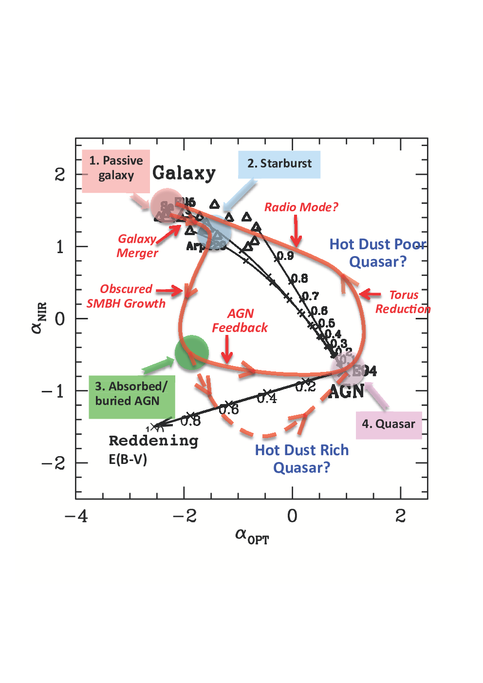
A family of possible evolutionary cycles could be drawn, varying the parameters of the initial merging (e.g. mass, gas fraction, accretion rate). A quantitative picture of the cosmic cycle (e.g. the duration of the duty cycle in each phase, the dependence on the initial conditions, etc.) could thus be obtained from the density of objects around the mixing diagram. These results, in turn, could put constraints on the physics adopted to model AGN/galaxy coevolution in numerical simulations. We plan to address the quantitative evolution of quasar-galaxy SEDs in the mixing diagram, over the complete cosmic cycle in later papers, including in the analysis of also type 2 AGN.
However, we have to note that Figure 13 is just an idealized illustration. The tracks of the evolution of sources could be very complicated and sources could evolve in various direction in the mixing region. Bongiorno et al. (2012) plotted all the XMM-COSMOS sources in the mixing diagram and there is no obvious accretion rate distribution correlated with different regions on the mixing diagram observed.
For a longer term study of the full evolutionary picture, the mixing diagram definition could be extended to other wavelengths. For example, we could investigate the optical to ultraviolet SED with respect to the near infrared SED for the extinction law; we could study the radio and far-infrared SED with respect to optical/near-infrared for the radio-loudness; we could check the ultraviolet SED with respect to X-ray for the . The multiwavelength analysis of the AGN emission could not only significantly improve our understanding of the SMBH accretion, the AGN structure and the unification of AGN, but also would help us understand the role of the SMBH in the co-evolution cosmic cycle.
Acknowledgments
HH thanks Belinda Wilkes, Martin J. Ward and Zhenyi Cai for valuable discussions. This work was supported in part by NASA Chandra grant number G07-8136A (HH, ME, CV). Support from the Italian Space Agency (ASI) under the contracts ASI-INAF I/088/06/0 and I/009/10/0 is acknowledged (AC and CV). MS acknowledges support by the German Deutsche Forschungsgemeinschaft, DFG Leibniz Prize (FKZ HA 1850/28-1). KS gratefully acknowledges support from Swiss National Science Foundation Grant PP00P2_138979/1.
References
- Alongi et al. (1993) Alongi, M., Bertelli, G., Bressan, A., Chiosi, C., Fagotto, F., Greggio, L., Nasi, E., 1993, A&AS, 97, 851
- Barvainis (1987) Barvainis, R. 1987, ApJ, 320, 537
- Bennert et al. (2010) Bennert, V. N., Treu, T., Woo, J.-H., Malkan, M. A., Le Bris, A., Auger, M. W., Gallagher, S., Blandford, R. D., 2010, ApJ, 708, 1507
- Bennert et al. (2011) Bennert, V. N., Auger, M. W., Treu, T., Woo, J.-H., Malkan, M. A., 2011, ApJ, 742, 107
- Bongiorno et al. (2007) Bongiorno, A., et al., 2007, A&A, 472, 443
- Bongiorno et al. (2012) Bongiorno, A., et al., 2012, MNRAS, 427, 3103
- Bouwens et al. (2012) Bouwens, R. J., et al., 2012, ApJ, 754, 83
- Brandt& Hasinger (2005) Brandt, W. N. & Hasinger, G. 2005, ARA&A, 43, 827
- Bressan et al. (1993) Bressan, A., Fagotto, F., Bertelli, G., Chiosi, C., 1993, A&AS, 100, 647
- Brusa et al. (2007) Brusa, M., et al., 2007, ApJS, 2007, 172, 353
- Brusa et al. (2010) Brusa, M., et al., 2010, ApJ, 716, 348
- Bruzual & Charlot (2003) Bruzual, G. & Charlot, S., 2003, MNRAS, 344, 1000
- Cai et al. (2013) Cai, Z., et al., 2013, ApJ, 768, 21
- Calzetti et al. (2000) Calzetti, D., Armus, L. Bohlin, R. C., Kinney, A. L., Koornneef, J., Storchi-Bergmann, T., 2000, ApJ, 533, 682
- Capak et al. (2007) Capak, P., et al., 2007, ApJS, 172, 99
- Cappelluti et al. (2007) Cappelluti, N., et al., 2007, ApJS, 172, 341
- Cappelluti et al. (2009) Cappelluti, N., et al., 2009, A&A, 497, 635
- Cardelli et al. (1989) Cardelli, J. A., Clayton, G. C., Mathis, J. S., 1989, ApJ, 345, 245
- Chabrier (2003) Chabrier, G., 2003, PASP, 115, 763
- Cirasuolo et al. (2007) Cirasuolo, M. et al. 2007, MNRAS, 380, 585
- Cisternas et al. (2011) Cisternas, M. et al. 2011, ApJ, 726, 57
- Civano et al. (2011) Civano, F., et al., 2011, ApJ, 741, 91
- Coleman et al. (1980) Coleman, G. D., Wu, C. C., & Weedman, D. W., 1980, ApJS, 43, 393
- Crenshaw & Kraemer (2001) Crenshsw D. M. & Kraemer S. B. 2001, ApJ, 562, L29
- Elvis et al. (1994) Elvis, M. et al., 1994, ApJS, 95, 1
- Elvis et al. (2012) Elvis, M. et al., 2011, ApJ, accepted, astro-ph/1209.1478
- Fabian et al. (2008) Fabian, A. C., Vasudevan, R. V., & Gandhi, P., 2008, MNRAS, 385, L43
- Fabian et al. (2009) Fabian, A. C., Vasudevan, R. V., Mushotzky, R. F., Winter, L. M., & Reynolds, C. S., 2009, MNRAS, 394, 89
- Ferrarese & Merrit (2000) Ferrarese, L. & Merrit, D. 2000 ApJ, 539, L9
- Fitzpatrick (1999) Fitzpatrick, E. L. 1999, PASP, 111, 63
- Fagotto et al. (1994a) Fagotto, F., Bressan, A., Bertelli, G., Chiosi, C., 1994a, A&AS, 104, 365
- Fagotto et al. (1994b) Fagotto, F., Bressan, A., Bertelli, G., Chiosi, C., 1994b, A&AS, 105, 29
- Franceschini et al. (1999) Franceschini, A., Hasinger, G., Miyaji, T., & Malquori, D., 1999, MNRAS, 310, L5
- Gallerani et al. (2005) Gallerani, S., et al., 2010, A&A, 523, 85
- Gebhardt et al. (2000) Gebhardt, K., et al. 2000, AJ, 539, L13
- Girardi et al. (1996) Girardi, L., Bressan, A., Chiosi, C., Bertelli, G., Nasi, E., 1996, A&AS, 117, 113
- Glikman et al. (2006) Glikman, E., Helfand, D. J., & White, R. L., 2006, ApJ, 640, 579
- Glikman et al. (2012) Glikman, E., et al. 2012, ApJ, 757, 51
- Gordon et al. (2003) Gordon, K. et al., 2003, ApJ, 594, 279
- Granato et al. (2004) Granato, G. L., De Zotti, G., Silva, L., Bressan, A., Danese, L., 2004, ApJ, 600, 580
- Hao et al. (2010) Hao, H., et al., 2010, ApJ, 724, L59
- Hao et al. (2011) Hao, H., et al., 2011, ApJ, 733, 108
- Hao et al. (2013a) Hao, H., et al., 2012a, MNRAS submitted, arXiv:1210.3033
- Hao et al. (2013b) Hao, H., et al., 2013b, ApJL, to be submitted
- Hasinger et al. (2007) Hasinger, G., et al., 2007, ApJS, 172, 29
- Ho (2008) Ho, L. C., 2008, ARA&A, 46, 475
- Hopkins et al. (2004) Hopkins, P. F., et al., 2004, AJ, 128, 1112
- Hopkins et al. (2006) Hopkins, P. F., et al., 2006, ApJS, 163, 1
- Hopkins et al. (2007) Hopkins, P. F., Richards, G. T., & Hernquist, L., 2007, ApJ, 654, 731
- Ilbert et al. (2009) Ilbert, O., et al., 2009, ApJ, 690, 1236
- Ilbert et al. (2010) Ilbert, O., et al., 2010, ApJ, 709, 644
- Jiang et al. (2010) Jiang, L. et al., 2010, Nature, 464, 380
- Kelly et al. (2007) Kelly, Brandon C. 2007, ApJ, 665, 1489
- Kewley et al. (2006) Kewley, L. J., Groves, B., Kauffmann, G., & Heckman, T., 2006, MNRAS, 372, 961
- Komatsu et al. (2009) Komatsu, E., et al., 2009, ApJS, 180, 330
- Kormendy & Richstone (1995) Kormendy, J. & Richstone, D. 1995, ARA&A, 33,581
- Lapi et al. (2006) Lapi, A., et al., ApJ, 650, 42
- Li et al. (2007) Li, Y., et al., 2007, ApJ, 665, 187
- Lilly et al. (2007) Lilly, S. J., et al., 2007, ApJS 172, 70
- Lilly et al. (2009) Lilly, S. J., et al., 2009, ApJS 184, 218
- Mainieri et al. (2007) Mainieri, V., et al., 2007, ApJS, 172, 368
- Maiolino et al. (2001) Maiolino, R., et al. 2001, A&A, 365, 28
- Malkan & Sargent (1982) Malkan, M. A., & Sargent, W. L. W., 1982, ApJ, 254, 22
- Mao et al. (2007) Mao, J., Lapi, A., Granato, G. L., De Zotti, G., Danese, L., 2007, ApJ, 667, 655
- Marconi & Hunt (2003) Marconi, A. & Hunt, L. K. 2003, ApJ, 589, L21
- McCracken et al. (2010) McCracken, H. J., et al., 2010, ApJ, 708, 202
- Merloni et al. (2010) Merloni, A., et al. 2010 ApJ 708, 137
- Merloni & Heinz (2012) Merloni, A., & Heinz, S., 2012, Planets, Stars and Stellar Systems, vol 6, ed W. Keel
- Misselt et al. (1999) Misselt, K. A., Clayton, G. C., Gordon, K. D., 1999, ApJ, 515, 128
- O’Brien et al. (1988) O’Brien, P. T., Wilson, R., & Gondhalekar, P. M. 1988, MNRAS, 233, 801
- O’Donnell (1994) O’Donnell, J. E., 1994, ApJ, 422, 158
- Polletta et al. (2007) Polletta, M., et al. 2007, ApJ, 663, 81
- Richards et al. (2003) Richards, G. T., et al. 2003, AJ, 126, 1131
- Richards et al. (2006) Richards, G. T. et al. 2006, ApJS, 166, 470
- Richstone et al. (1998) Richstone, D., et al. 1998, Nature, 395, 14
- Salvato et al. (2009) Salvato, M. et al. 2009 ApJ 690, 1250
- Sandage et al. (1971) Sandage, A. 1971 SWNG conf, 271
- Sanders et al. (1989) Sanders, D. B., Phinney, E. S., Neugebauer, G., Soifer, B. T., & Matthews, K. 1989, ApJ, 347, 29
- Schawinski et al. (2009) Schawinski, K., et al., 2009, ApJL, 692, 19
- Schmidt & Green (1983) Schmidt, M. & Green, R. F. 1983, ApJ, 269, 352
- Schneider et al. (2007) Schneider, D. P. et al. 2007, AJ, 134, 102
- Schramm & Silverman (2013) Schramm, M. & Silverman, J. D., 2013, ApJ, 767, 13
- Scoville et al. (2007) Scoville, N. Z., et al., 2007, ApJS, 172, 1
- Shang et al. (2011) Shang, Zhaohui, et al., 2011, ApJS, 196, 2
- Sikora et al. (2007) Sikora, M., Stawarz, L. & Lasota, J. P., 2007, ApJ, 658, 815
- Silva et al. (1998) Silva, L., Granato, G. L., Bressan, A., & Danese, L. 1998, ApJ, 509, 103
- Silverman et al. (2005) Silverman, J. D. et al. 2005, ApJ, 624, 630
- Soltan (1982) Soltan, A., 1982, MNRAS, 200, 115
- Taniguchi (1999) Taniguchi, Y. 1999, ApJ, 524, 65
- Trump et al. (2009) Trump, J. R. et al. 2009 ApJ, 696, 1195
- Trump et al. (2011) Trump, J. R. et al. 2011 ApJ, 733, 60
- Vasudevan et al. (2009) Vasudevan, R. V., Mushotzky, R. F., Winter, L. M., & Fabian, A. C. 2009, MNRAS, 399, 1553
- Vestergaard & Peterson (2006) Vestergaard, M. & Peterson, B. M. 2006 ApJ 641, 689
- Ueda et al. (2003) Ueda, Y. et al. 2003 ApJ 598, 886
- Ward et al. (1987) Ward, M. et al. 1987 ApJ, 315, 74
- Weedman (1973) Weedman, D. 1973 ApJ, 183, 29
- Wild et al. (2010) Wild, V., et al., 2010, MNRAS, 405, 933
- Wills, Netzer & Wills (1985) Wills, B. J., Netzer, H., & Wills, D. 1985, ApJ, 288, 94
- Xiao et al. (2012) Xiao, T., et al. 2012, MNRAS, 421, 486
- Young et al. (2008) Young, M., Elvis, M., & Risaliti, G. 2008, ApJ, 688, 128