Suitability of hybrid gravitational waveforms for unequal-mass binaries
Abstract
This article studies sufficient accuracy criteria of hybrid post-Newtonian (PN) and numerical relativity (NR) waveforms for parameter estimation of strong binary black-hole sources in second-generation ground-based gravitational-wave detectors. We investigate equal-mass non-spinning binaries with a new 33-orbit NR waveform, as well as unequal-mass binaries with mass ratios and . For equal masses, the 33-orbit NR waveform allows us to recover previous results and to extend the analysis toward matching at lower frequencies. For unequal masses, the errors between different PN approximants increase with mass ratio. Thus, at 3.5PN, hybrids for higher-mass-ratio systems would require NR waveforms with many more gravitational-wave (GW) cycles to guarantee no adverse impact on parameter estimation. Furthermore, we investigate the potential improvement in hybrid waveforms that can be expected from 4th order post-Newtonian waveforms, and find that knowledge of this 4th post-Newtonian order would significantly improve the accuracy of hybrid waveforms.
I Introduction
Within the next few years, Advanced LIGO [1, 2, 3], Virgo [4], and LCGT [5] will likely observe the first gravitational wave signals. The detection rate is expected to be somewhere between 0.4 and 1000 detections per year for binary black-hole (BBH) systems with masses below 100 at distances of several gigaparsecs [6]. Because the gravitational wave (GW) signals will be faint compared to the detector noise, accurate source modeling of the predicted GWs will be necessary to detect signals and perform parameter estimation on them via matched filtering.
Several methods have been developed to calculate the GWs from a BBH system, two of which are post-Newtonian (PN) theory and Numerical Relativity (NR). The PN expansion [7] is a slow-motion, weak-field approximation to General Relativity, and it provides an accurate description of the inspiral prior to merger, but becomes increasingly inaccurate close to merger. NR can be used to model the late inspiral, merger, and ringdown of a BBH evolution, but at high computational cost [8, 9].
In order to use the best features of each type of model, one stitches a long PN inspiral to the front of an NR waveform of the late inspiral, merger, and ringdown, thus creating a hybrid waveform. The trick is to stitch the NR and PN parts together such that the error due to higher-order unknown terms in the PN waveform is small, while necessitating as few NR orbits as possible to reduce the computational cost. This has been explored in our previous work [10] for equal-mass, non-spinning binaries, and also in [11, 12, 13, 14].
Hybrid gravitational waveforms have many uses. They play an important role in the creation of phenomenological waveforms [15, 11], which are used in template banks for event detection. In addition, hybrids are used within the NINJA project [16, 17, 18] in order to test the GW search pipeline for ground-based detectors.
A sufficient criterion to determine whether PN+NR hybrid waveforms are suitable for parameter estimation in the advanced detector era is that a GW model must be deemed indistinguishable from the true waveform within the Advanced LIGO noise spectrum. That is, we place upper bounds on the error measure (to be defined in Sec. II.4), where . This error measure is distance-independent as long as cosmological redshifts are neglible.
This paper extends our earlier analysis in several directions: First, we calculate for equal-mass hybrids constructed from a previously unpublished 33-orbit NR waveform in order to confirm results obtained with the 15-orbit NR used in prior works. Second, we extend the parameter space to hybrid waveforms from unequal-mass binaries by calculating this error in the most demanding usage case of parameter estimation. Third, we examine the possibility of decreasing hybrid errors if PN were known to 4th order. A decrease in PN error would mean that more accurate hybrid waveforms could be created with the current length NR waveforms, thus decreasing the computational cost of generating these templates.
This paper is organized as follows: Section II reviews the methodology of our analysis, including the types of PN and NR waveforms, the hybridization procedure and how the errors are quantified. Section III extends our earlier results in [10] and [19] using a new 33-orbit NR waveform. Section IV applies our error analysis to unequal-mass binaries. Finally, section V estimates the errors one would obtain for PN+NR hybrids if the 4PN terms were known.
II Methodology
II.1 Post-Newtonian waveforms
Post-Newtonian (PN) theory presents a slow-motion, weak-field approximation to General Relativity in terms of expansions of and . We use the same PN approximants as in our previous work [10]. Specifically, we investigate the properties of TaylorT1, TaylorT2, TaylorT3, and TaylorT4 (as defined in [20, 21, 19]) to 3.5PN order in phase and 3.0PN order in amplitude [22, 23, 24, 25, 26, 27, 28, 29]. These four approximants differ only in their unknown higher-order PN terms. As in [10], we consider the (2,2) mode of the spin-weight spherical-harmonic decomposition of the gravitational waveform. The amplitude of the PN waveform of this mode is always used at 3PN order, except for Fig. 3 which uses the amplitude to 2.5PN order for consistency with earlier work [19].
II.2 Numerical waveforms
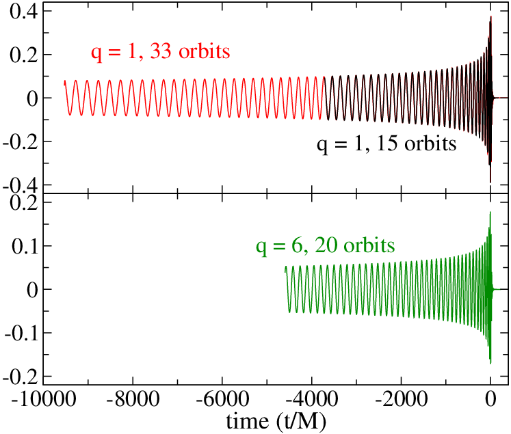
The numerical relativity waveforms were produced with the SpEC code [30], a multi-domain pseudospectral code to solve Einstein’s equations. We use two simulations for the equal-mass, non-spinning binaries. One of these two simulations covers 15 orbits; it was presented in Refs. [19, 31] and was compared to independently computed equal-mass zero-spin BBH waveforms in [32, 33]. This 15-orbit waveform was already used in the preceding study in MacDonald et al.\xspace [10]. The second equal-mass, non-spinning waveform covers 33 inspiral orbits. This is a new simulation which is part of a larger, ongoing parameter-space study of binary black holes [34]. This waveform was obtained with numerical techniques similar to those of [35]. The trajectories of the black holes in the 33-orbit simulation are shown in Fig. 1, and the corresponding gravitational waveform in the top panel of Fig. 2. It is more than twice the length of the 15-orbit waveform, and will allow us to reduce the GW matching frequency from to where with and the individual masses of the black holes. In this paper, all frequencies refer to the gravitational-wave frequency that is extracted from the mode of the gravitational waveform; at leading order, this frequency differs by a factor of two from the orbital frequency often used in PN calculations.

II.3 Hybridization Procedure
The hybridization procedure used for this investigation was the same as in our previous work (see Sec. 3.3 of [10]): The PN waveform, , is time and phase shifted to match the NR waveform, , and they are smoothly joined together in a GW frequency interval centered at with width :
| (1) |
This translates into a matching interval because the GW frequency continuously increases during the inspiral of the binary. As argued in [10], we choose because it offers a good compromise of suppressing residual oscillations in the matching time, while still allowing to be matched as closely as possible to the beginning of .
The PN waveform depends on a (formal) coalescence time, , and phase, . These two parameters are determined by minimizing the GW phase difference in the matching interval as follows:
| (2) |
where and are the time and phase parameters for the best matching between and , and is the phase of the (2,2) mode of the gravitational radiation. (Because we consider only the (2,2) mode, this procedure is identical to time and phase shifting the PN waveform until it has best agreement with NR as measured by the integral in Eq. 1) The hybrid waveform is then constructed in the form
| (3) |
where is a blending function defined as
II.4 Quantifying errors
As in [10], the error measurement used to determine the indistinguishability of two hybrid waveforms within a gravitational wave detector’s noise spectrum was , or the noise-weighted inner product of the difference between the two hybrids. We denote this difference , where and are two hybrid waveforms to be compared. The norm is defined through the noise-weighted inner product
| (8) |
where and are the Fourier transforms of two waveforms and . denotes the (one-sided) power spectral density,
| (9) |
where is the noise correlation matrix for zero-mean, stationary noise. As in our previous work, we calculate these errors using the Advanced LIGO noise curve in its high-power, zero-detuned configuration (ZERO_DET_high_P in [36]).
In order to reduce the effects of the Gibbs phenomenon in the Fourier transforms, we apply a Planck-taper window function [37] to the time-domain data before computing the Fourier transform. The error is then minimized by a time and phase shift of one waveform relative to the other.
Sufficient accuracy of the model waveform is guaranteed if [38]
| (10) |
Here, is a bound on the fractional signal-to-noise ratio (SNR) loss while searching for GW signals. We follow the suggestion in [38] and consider . The parameter in Eq. (10) represents an effective SNR that incorporates a safety factor [39], the impact of a network of detectors, and SNR of the GW event. It is defined as
| (11) |
where is the number of detectors. As in [10], we indicate and in the plots below to cover the range of possibilities with a strong GW signal and a single to many detectors. In addition, the event-detection limit of Eq. (10), , can be rewritten in terms of . We also indicate this bound in our figures.
III RESULTS: equal-mass, non-spinning binaries

As a first consistency check, we perform a PN comparison similar to Boyle et al.\xspace [19]. That work compared a 15-orbit NR waveform to the PN approximants Taylor T1, T2, T3, and T4. PN and NR waveforms were matched at a certain GW frequency , and then the differences in phases between the two waveforms were computed as well as the relative amplitude error. We repeat this analysis for the Taylor T3 3.5/2.5PN waveform to see if the same behaviour holds for a longer numerical waveform. The results are shown in Fig. 3. As in [19], we matched the NR and PN waveforms together at 0.040, 0.050, and 0.063, but also at the lower frequencies 0.025 and 0.030.
The solid lines in Fig. 3 show the phase error obtained when using the new 33-orbit NR waveform. The dashed lines show the results from [19]. Agreement between these two comparisons is excellent, demonstrating that extending the SpEC simulations to larger numbers of orbits yields consistent results with using a shorter waveform. This comparison validates the earlier results [19], and our matching procedure, and demonstrates consistency between the 15- and 33-orbit simulations.

Continuing the consistency tests between the 15-orbit waveform [19, 31] and the new 33-orbit waveform presented in Sec. II.2, Fig. 4 shows the error between hybrids created with the two numerical waveforms matched at the same hybridization frequency as a function of total mass, as well as the error between the high and medium resolutions for each waveform. This figure shows first that the error between hybrids created with the longer and shorter NR waveforms is comparable to the numerical error of either simulation. Numerical errors are much smaller than the error bound for , and so we shall therefore disregard numerical errors.

Having established the accuracy of the 33-orbit waveform, let us now assess the quality of PN-NR hybrid waveforms at the lower matching frequencies that are made accessible by this NR waveform. We choose several matching frequencies in the interval , and for each of these, we construct hybrid waveforms with Taylor T1, T2, T3, and T4. We then compute pairwise differences at a fixed total mass using the ZERO_DET_HIGH_P LIGO noise-curve [36]. The results of this comparison are shown as the solid lines in Fig. 5. Differences decrease with decreasing matching frequency (i.e., when switching from PN to NR earlier), as one would expect. The thick dashed lines represent the same comparison performed with the 15-orbit waveform, i.e., the precise data already presented in Ref. [10]. The comparisons agree for , where both NR waveforms are available. Furthermore, the long waveform continues the trend set by the earlier, shorter waveform without surprises. This indicates that extrapolating errors in our analyses to lower matching frequencies is indeed valid. It also indicates that there is no unexpected behaviour of PN or NR in the newly accessible GW frequency interval , with PN and NR converging toward each other.
IV Unequal-mass black holes
Now let us consider binary black-hole systems with mass ratio . As increases, the inspiral proceeds more slowly, in proportion to the symmetric mass ratio (see e.g., post-Newtonian expansions [7]). This is illustrated by Fig. 6, which shows the number of inspiral orbits to merger as a function of gravitational wave frequency. This figure was created by plotting the number of orbits prior to the maximum amplitude of hybrid waveforms matched at the earliest possible GW frequency ( for and 0.042 for ) with a Taylor T4 waveform against .
Starting from the same GW frequency (e.g., ), the binary proceeds through roughly twice as many orbits. Conversely, the same number of orbits to merger (e.g., ) occurs at higher frequency for than for . The dashed lines indicate a matching frequency of and 12 orbits; we will use these two reference values in subsequent comparisons. Because unequal-mass binaries spend more orbits in the strong field regime, we would expect that with increasing mass ratio , hybrids need to be matched a larger number of orbits before merger than for . The next sections will quantify this expectation.
Before proceeding, it is important to note that the error between hybrids constructed with different PN approximants is much higher than the numerical error of the NR waveforms. We performed an analysis similar to that in Fig. 4, where the highest resolution NR waveform was compared to the medium resolution waveform for all mass ratios used in this paper. In all cases, the numerical error is about an order of magnitude smaller than the PN error in hybrid waveforms.

IV.1 Phase errors between PN and NR
Let us start with investigating the phase difference between NR and PN with measures that are independent of the LIGO noise spectrum. We calculate the accumulated phase difference between PN and NR waveforms. Following Hannam et al.\xspace [40], we match PN and NR at and then calculate their phase difference at a certain time before this matching point.
We perform this computation for TaylorT1, TaylorT2, TaylorT3, and TaylorT4. (The TaylorT3 waveform was only calculated to 3.0PN order in phase since the 3.5PN order waveform does not reach .) The results are shown in Fig. 7. The top panel shows the phase difference between PN and NR at 8 GW cycles before (equivalent to Fig. 8 of [40]), and the bottom panel shows the phase difference at for PN and NR waveforms matched in phase at . Both panels show similar trends. In the lower panel, the phase difference increases more rapidly with increasing mass ratio because the number of orbits within the comparison increases with increasing mass ratio (7.4 orbits for versus 12.2 orbits for ).
Our findings disagree with the results of Hannam et al.\xspace [40], despite following the identical comparison protocol. Figure 8 of [40] shows a roughly constant phase difference between TaylorT1 and the numerical simulation of radians, for all considered mass ratios (), whereas we find a steadily declining phase difference reaching zero near . Similar trends hold for TaylorT4: Ref. [40] reports phase differences radians for mass ratios . We see a very small phase difference at mass ratio , and steadily increasing phase differences at larger mass ratios. These discrepancies are caused by an error in the numerical setup of the simulations used in Ref. [40]11 1 M. Hannam, S. Husa, and M. Pürrer (private communication, October 29, 2012).


Figure 7 shows that one cannot assume that any single PN approximant will be suitable for all of parameter space. Phase errors between PN and NR change dramatically with increasing mass ratio. The agreement between TaylorT4 and NR waveforms in the case of equal-mass non-spinning binaries, for example, is purely coincidental. As the mass ratio of the binary increases, this phase error becomes much larger for TaylorT4, and in fact becomes smaller for TaylorT1 and TaylorT2. Because the Taylor approximants differ only in higher order post-Newtonian terms, the spread between them can be taken as a measure of the post-Newtonian truncation error. For the comparison in the top panel, this indicates a post-Newtonian truncation error of radians for increasing to radian for . Within this (admittedly large) truncation error, all four Taylor approximants are consistent with the numerical data (i.e., consistent with zero phase difference).
IV.2 Hybrid errors
We now repeat the analysis of Fig. 5 for binaries with higher mass ratios: We hybridize TaylorT[1,2,3,4] at several matching frequencies . At each , we compute differences between all six pairs of PN approximants and plot these differences as a function of . The results are shown in Fig. 8 for mass ratio and for total masses 10 and 40. represents a binary with component masses 1.67 and 8.33, which we shall take as an approximation of a black-hole–neutron-star (BH-NS) binary. results in component masses 6.67 and 33.337, a BBH system where the smaller black hole is consistent with known black-hole masses. We chose these masses because they are more astrophysically probable for this mass ratio than the total mass of 20 that we used for . The coloured lines represent the differences between hybrids as just described. To ease the comparison with the results of Fig. 5, we duplicate those data into Fig. 8 as the grey lines in the background.
One notices immediately two differences between and : (1) At the same matching frequency, results in larger differences. This might be caused by the larger number of orbits that the binary spends at high frequency cf. Fig. 6. (2) The comparison covers only comparatively high matching frequencies , whereas the comparison reaches much lower frequencies. This originates in the slower inspiral of higher mass ratios (i.e., longer time to merger from the same starting frequency) and the higher computational cost of high mass ratio simulations.
The difference between the TaylorT1 and TaylorT2 hybrids is particularly small in Fig. 8. This is consistent with Fig. 7, where for , the differences between PN and NR are similar for these two approximants.

Let us now investigate the dependence on in more detail. We compute the differences for all mass ratios at the same matching frequency (the data for and 6 can be read off of Figs. 5 and 8, respectively). The upper panel of Fig. 9 shows these differences as a function of . Once again, it is evident that differences increase with mass ratio.
Length requirements for NR waveforms are often phrased in the convenient unit “number of NR orbits”. To place this notion in context, we match PN+NR 12 orbits before merger, compute differences , and plot these in the lower panel of Fig. 9. When matching a fixed number of orbits before merger, increases even more steeply with , because the matching frequency increases with , cf. Fig. 6.


Both Figs. 7 and 9 show that the error between hybrids using different PN approximants increases with mass ratio. Therefore, with increasing mass ratio binaries, NR waveforms will have to be longer to create hybrids of similar quality. For mass ratio 6, one might estimate from Fig. 8 that total mass requires a matching frequency of . The matching interval Eq. (1) would then extend to a lower frequency requiring about 40 orbits covered by NR. The needed matching frequency (and thus the number of orbits) depends on the total mass considered; for , convergence of the errors with decreasing is not yet apparent (see the curves in Figure 8), so the NR waveform is too short to even estimate how long it should be. This indicates that BH-NS systems may very well place the most stringent requirements on NR simulations. (A proper treatment of BH-NS systems, of course, will also require to simulate the neutron star directly, including its tides and other effects arising from micro-physics. Such a simulation would be yet more challenging than our approach of using the easier BBH system as a proxy.)
It is no surprise that the error for hybrids matched at a certain or at a fixed number of orbits before merger would increase with mass ratio since the number of orbits spent in the strong field regime increases with mass ratio.
V Higher-order Post-Newtonian
The primary source of error lies in the truncation error of the PN approximants. Work is currently being done to calculate PN to 4th order [41, 42], therefore, an interesting question arises: how much might higher PN orders improve the accuracy of PN+NR hybrid waveforms? To address this question we consider the TaylorT4 approximant, where the phase evolution is determined by a single Taylor series [43]:
| (12) | |||||
Here, denotes the symmetric mass ratio, is Euler’s constant, is the speed of light, is the gravitational constant, and .

In Eq. 12, we have included the terms , , and at 4th through 5th PN order. These terms are currently unknown, but trends in the known coefficients can be used to approximate the magnitude of the unknown coefficients. Figure 10 plots the known coefficients vs. PN order for mass ratios . The figure also shows the coefficients for the test-mass limit , which are known up to 5.5-th PN order [44]. The coefficients behave rather erratically, but overall, they seem to be exponentially increasing, as indicated by the black line with filled circles. This black line represents , with a doubling of the coefficients with each increase in PN order (and halving with each decrease). Therefore, we shall take the unknown coefficients to be , and . These values are of course not the correct ones, but are indicative of the expected magnitudes of these coefficients. Hence, we will not be able to compute the correct 4PN (and higher) PN waveforms, but merely estimate the errors in those waveforms, were the coefficients known.
Assuming , we can estimate the truncation error of 3.5PN TaylorT4 by computing between the standard TaylorT4 (with for ) and a modified TaylorT4 with . This comparison is shown as the blue curve in Fig. 11 which is labeled “3.5PN” (the label indicates that this is an estimate of the error of 3.5PN order). This new estimate of the 3.5PN truncation error should of course be consistent with our earlier estimates shown in Fig. 5. To demonstrate this consistency, we include the data of Fig. 5 as the greyed out lines in the background of Fig. 11. Indeed, the new estimate (“3.5PN”) follows closely the trends of the more exhaustive study, lending confidence in this approach.
Repeating this procedure at next higher PN order will now result in an error estimate of 4PN (were it known). Thus we compare TaylorT4 hybrids with and without the term. This results in the red line labeled “4PN” in Fig. 11. We can go one PN order further, and include an term (resulting in the line labeled “4.5PN”). We can also remove the (known) 3.5 PN term, to estimate the 3PN truncation error if 3.5PN were not known (the curve labeled “3PN”; this curve compares with ).
We repeated this analysis for the mass ratios and 6. The results are similar to the calculation of Fig. 11; as an example, Fig. 12 presents the analogous calculation for . In Fig. 11 and 12, a clear pattern emerges: Each additional PN order reduces by approximately a factor of . When matched at low frequency (where PN is more accurate) the reduction in error is somewhat faster than when matching at high frequency. To make these statements quantitative, Figure 13 plots the ratio of the “3.5PN” and the “4PN” curves in Fig. 11 and 12. It also shows data for the remaining mass ratios (). This ratio is at and drops to at the lowest accessible matching frequency . The gain of higher-order PN is approximately independent of mass ratio, except for high matching frequencies and high mass ratios; in this regime errors are so large that the asymptotic trends for small errors/early matching are masked.


V.1 3PN Hybrids
To further quantify the reliability of our estimate of 4PN improvements, let us apply our analysis to 3PN waveforms. The 3PN truncation error estimate based on modifying the 3.5PN coefficient is already plotted in Figs. 11 and 12. What remains is the equivalent of Fig. 5 at 3PN order: We prepare TaylorT[1,2,3,4] hybrids at 3PN order, and compute their pairwise differences. This results in the thick solid blue lines of Fig. 14. Compared to the 3.5PN comparison of Fig. 5 (replicated in the grey lines in Fig. 14), the error of 3PN is indeed somewhat larger than for 3.5PN. The change in error 3PN vs. 3.5PN is smaller than the factor of 2 we would have predicted from Fig. 11, presumably because the actual coefficient is smaller than the assumed of Fig. 10.

Fig. 14 offers another cautionary lesson: Consider the differences between hybrids using the 3PN Taylor T2,T3,T4 approximants. There are three such differences, plotted with blue dashed lines in Fig. 14. The differences between these three hybrids are surprisingly small, with , even when hybridized at the very large matching frequency . If one had used only these three approximants, and if only 3PN were available, one would have concluded that the resulting hybrids are good for Advanced LIGO purposes, and that short NR simulations are sufficient.
But this conclusion would have been entirely incorrect! The dotted red lines in Fig. 14 show the difference between 3PN hybrids with the 3.5PN TaylorT4 hybrid. These differences are an order of magnitude larger than the 3PN internal TaylorT2, T3, and T4 differences. At 3PN, TaylorT2, T3, and T4 are very similar, and they are all three off by the same large amount. The 3PN TaylorT1 comparisons reveal this effect: As shown by the solid blue lines in Fig. 14, differences between TaylorT1 hybrids and the other three hybrids are all very large. As this analysis demonstrates, these large differences are not caused by a “deficiency” of TaylorT1, but rather by coincidentally similar deviations from the true waveform in the TaylorT2,3,4 approximants. The same effect at 3.5PN order is apparent in Fig. 5: At low matching frequencies, the pairwise differences between TaylorT2,3,4 are significantly smaller than the differences relative to TaylorT1. Therefore, it is important to investigate many different approximants, and not to discount lone outliers as in Fig. 14.
VI Discussion
In this paper, we have presented an analysis of errors that affect hybrid gravitational waveforms for a range of mass ratios to assess their suitability for parameter estimation with Advanced LIGO. We have also estimated by how much these errors would be reduced if PN were known to a higher order.
In the case of equal-mass, non-spinning binaries, we have found that the results obtained with the most recent, 33-orbit numerical waveform are consistent with previous results obtained using the older, shorter 15-orbit simulation. The errors between hybrids using these two NR waveforms are small enough for parameter estimation for sources with . In addition, when compared to PN, these two NR waveforms yield similar results. The results in Fig. 5 show that the results using the 15-orbit waveform can be reproduced and extended.
Expanding the parameter space to unequal-mass binaries, we have found that PN errors grow with increased mass ratio as observed by [13, 12, 14, 11]. Phase differences between PN and NR vary strongly with mass ratio and PN approximant. Therefore, no single PN waveform is appropriate for all of parameter space. For example, despite the fact that Taylor T4 matches remarkably well with NR in the case of equal-mass, non-spinning binaries, this is no longer true as the mass ratio between the black holes in the binary system increases. It is only a coincidence that TaylorT4 and NR are so similar in this very unique configuration. In fact, for , TaylorT1 and TaylorT2 agree very well with NR, whereas TaylorT4 does not, cf. Fig. 7.
When evaluating for hybrids which use different PN approximants, it becomes clear that higher mass ratio binaries will require increasingly more NR orbits to reach similar accuracy. This becomes problematic for high mass ratio binaries, since they are more computationally expensive because it requires more numerical resolution to resolve the smaller black hole. We also note the recent analysis [45] of an equal-mass aligned spin BBH simulation with very large spins. Ref. [45] found that the simulation covering orbits was of insufficient length to reliably hybridize with PN.
Knowledge of higher-order PN waveforms will significantly improve the quality of PN+NR hybrid waveforms. As demonstrated in Figs. 11 and 12, any further additional PN order should decrease errors in our measure by roughly a factor of , for the same length of the NR waveform. Because mismatches are proportional to the square of this will reduce mismatches by a factor . For a specified accuracy, the knowledge of a higher-order PN expansion would allow one to shorten the length of NR simulations. For , Fig. 11 indicates that the matching frequency could be raised from to , thus approximately reducing the temporal length of the NR simulation by a factor of . This would be a substantial saving for future NR simulations. We emphasize that these estimates depend on our assumption of the approximate magnitude of the unknown PN coefficients, as discussed in the context of Fig. 10.
This analysis has also provided us with an important cautionary tale: one cannot ignore outliers when comparing many different PN approximants to each other. This is illustrated in the 3PN case in Fig. 14, where the error between Taylor T2, T3, and T4 hybrids is very small, but when compared to Taylor T1 hybrids, the error is much higher. Thus, it is very important, when doing this type of analysis, to consider as many different PN approximants as possible.
This work could be extended in a few ways. First of all, it would be interesting to further extend the parameter space to spinning binaries, and also to the most general case of precessing binaries. Some work has been done to create hybrids for precessing binaries in [46, 47, 48, 49], but error estimates on this type of hybrid are still a ways off. It would also be useful to extend the error analysis of GW modes to modes different from just the (2,2) mode, because these other modes become increasingly important with higher mass ratio (e.g., [35]) and with precession of the orbital plane (e.g., [43, 50]).
It would also be useful to refine our error limit in Eq. 10 to incorporate the effects of a network of detectors in a more effective way. It might be worthwhile to have an error limit which depends on the total mass of the binary as in [13], or to consider some better way of finding an upper bound on . An important consideration is the fact that our error criterion is sufficient but not necessary to the suitability of these hybrid waveforms. For instance, investigations into detection efficiency of hybrid waveforms [51, 14] indicate that hybrid waveforms can be perfectly usable, even when failing the indistinguishability test by a wide margin.
Acknowledgements.
We would like to thank Mark Hannam, Sascha Husa, and Ulrich Sperhake for useful discussions, and thank Riccardo Sturani, Stefano Foffa, Luc Blanchet, Chad Galley, Alessandra Buonanno, and Samaya Nissanke for insights into the difficulties in computing higher order post-Newtonian expansions. The numerical waveforms used in this work were computed with the SpEC code [30]. We gratefully acknowledge support from the NSERC of Canada, from the Canada Research Chairs Program, from the Canadian Institute for Advanced Research, and from the Sherman Fairchild Foundation; from NSF grants PHY-0969111 and PHY-1005426 at Cornell, and from NSF grants PHY-1068881 and PHY-1005655 at Caltech. Computations were performed on the Zwicky cluster at Caltech, which is supported by the Sherman Fairchild Foundation and by NSF award PHY-0960291; on the NSF XSEDE network under grant TG-PHY990007N; and on the GPC supercomputer at the SciNet HPC Consortium [52]. SciNet is funded by: the Canada Foundation for Innovation under the auspices of Compute Canada; the Government of Ontario; Ontario Research Fund–Research Excellence; and the University of Toronto.References
- [1] B. Abbott et al. (LIGO Scientific Collaboration), Rept. Prog. Phys. 72, 076901 (2009), arXiv:0711.3041 [gr-qc] .
- [2] D. Shoemaker (the Advanced LIGO Team), “Advanced LIGO Reference Design,” (2009), [LIGO-M060056].
- [3] G. M. Harry (for the LIGO Scientific Collaboration), Class. Quantum Grav. 27, 084006 (2010).
- [4] The Virgo Collaboration, “Advanced Virgo Baseline Design,” (2009), [VIR-0027A-09].
- [5] K. Kuroda and the LCGT Collaboration, Class. Quantum Grav. 27, 084004 (2010).
- [6] J. Abadie et al. (LIGO Scientific), Class. Quant. Grav. 27, 173001 (2010), arXiv:1003.2480 [Unknown] .
- [7] L. Blanchet, Living Rev.Rel. 9, 4 (2006).
- [8] J. Centrella, J. G. Baker, B. J. Kelly, and J. R. van Meter, Rev. Mod. Phys. 82, 3069 (2010).
- [9] H. P. Pfeiffer, Class.Quant.Grav. 29, 124004 (2012), arXiv:1203.5166 [gr-qc] .
- [10] I. MacDonald, S. Nissanke, and H. P. Pfeiffer, Class. Quantum Grav. 28, 134002 (2011), arXiv:1102.5128 [gr-qc] .
- [11] L. Santamaría, F. Ohme, P. Ajith, B. Brügmann, N. Dorband, M. Hannam, S. Husa, P. Mösta, D. Pollney, C. Reisswig, E. L. Robinson, J. Seiler, and B. Krishnan, Phys. Rev. D 82, 064016 (2010), arXiv:1005.3306 [gr-qc] .
- [12] M. Hannam, S. Husa, F. Ohme, and P. Ajith, Phys. Rev. D 82, 124052 (2010), arXiv:1008.2961 [gr-qc] .
- [13] M. Boyle, Phys. Rev. D 84, 064013 (2011).
- [14] F. Ohme, M. Hannam, and S. Husa, Phys. Rev. D 84, 064029 (2011).
- [15] P. Ajith, S. Babak, Y. Chen, M. Hewitson, B. Krishnan, A. M. Sintes, J. T. Whelan, B. Brügmann, P. Diener, N. Dorband, J. Gonzalez, M. Hannam, S. Husa, D. Pollney, L. Rezzolla, L. Santamaría, U. Sperhake, and J. Thornburg, Phys. Rev. D 79, 129901 (2009).
- [16] The NINJA collaboration, http://www.ninja-project.org/.
- [17] B. Aylott et al., Class. Quantum Grav. 26, 165008 (2009), arXiv:0901.4399 .
- [18] P. Ajith, M. Boyle, D. A. Brown, B. Brugmann, L. T. Buchman, et al., Class. Quantum Grav. 29, 124001 (2012).
- [19] M. Boyle, D. A. Brown, L. E. Kidder, A. H. Mroué, H. P. Pfeiffer, M. A. Scheel, G. B. Cook, and S. A. Teukolsky, Phys. Rev. D 76, 124038 (2007).
- [20] T. Damour, B. R. Iyer, and B. S. Sathyaprakash, Phys. Rev. D 63, 044023 (2001), erratum: [53].
- [21] A. Buonanno, G. B. Cook, and F. Pretorius, Phys. Rev. D 75, 124018 (2007), arXiv:gr-qc/0610122 [gr-qc] .
- [22] L. Blanchet, G. Faye, B. R. Iyer, and B. Joguet, Phys. Rev. D 65, 061501 (2002), erratum: [23].
- [23] L. Blanchet, G. Faye, B. R. Iyer, and B. Joguet, Phys. Rev. D 71, 129902 (2005a).
- [24] L. Blanchet, B. R. Iyer, and B. Joguet, Phys. Rev. D 71, 129903 (2005b).
- [25] L. Blanchet, A. Buonanno, and G. Faye, Phys. Rev. D 74, 104034 (2006).
- [26] L. Blanchet, A. Buonanno, and G. Faye, Phys. Rev. D 75, 049903 (2007).
- [27] L. E. Kidder, Phys.Rev. D77, 044016 (2008), arXiv:0710.0614 [gr-qc] .
- [28] K. G. Arun, A. Buonanno, G. Faye, and E. Ochsner, Phys. Rev. D 79, 104023 (2009), arXiv:0810.5336 [gr-qc] .
- [29] L. Blanchet, A. Buonanno, and G. Faye, Phys. Rev. D 81, 089901 (2010).
- [30] http://www.black-holes.org/SpEC.html.
- [31] M. A. Scheel, M. Boyle, T. Chu, L. E. Kidder, K. D. Matthews and H. P. Pfeiffer, Phys. Rev. D 79, 024003 (2009), arXiv:gr-qc/0810.1767 .
- [32] M. Hannam, S. Husa, J. G. Baker, M. Boyle, B. Bruegmann, T. Chu, N. Dorband, F. Herrmann, I. Hinder, B. J. Kelly, L. E. Kidder, P. Laguna, K. D. Matthews, J. R. van Meter, H. P. Pfeiffer, D. Pollney, C. Reisswig, M. A. Scheel, and D. Shoemaker, Phys. Rev. D 79, 084025 (2009), arXiv:arXiv:0901.2437 [gr-qc] .
- [33] B. Garcia, G. Lovelace, L. E. Kidder, M. Boyle, S. A. Teukolsky, et al., (2012), accepted for publication in Phys. Rev. D, arXiv:1206.2943 [gr-qc] .
- [34] A. H. Mroue and H. P. Pfeiffer, (2012), arXiv:1210.2958 [gr-qc] .
- [35] L. T. Buchman, H. P. Pfeiffer, M. A. Scheel, and B. Szilagyi, Phys. Rev. D 86, 084033 (2012), arXiv:1206.3015 [gr-qc] .
- [36] D. Shoemaker (LIGO Collaboration), “Advanced LIGO anticipated sensitivity curves,” (2010), LIGO Document T0900288-v3.
- [37] D. McKechan, C. Robinson, and B. Sathyaprakash, Class.Quant.Grav. 27, 084020 (2010), arXiv:1003.2939 [gr-qc] .
- [38] L. Lindblom, B. J. Owen, and D. A. Brown, Phys. Rev. D 78, 124020 (2008), arXiv:0809.3844 [gr-qc] .
- [39] T. Damour, A. Nagar, and M. Trias, Phys. Rev. D 83, 024006 (2011), arXiv:1009.5998 [gr-qc] .
- [40] M. Hannam, S. Husa, F. Ohme, D. Müller, and B. Brügmann, Phys. Rev. D 82, 124008 (2010), arXiv:1007.4789 .
- [41] P. Jaranowski and G. Schafer, “Towards the 4th post-Newtonian Hamiltonian for two-point-mass systems,” (2012), arXiv:1207.5448 [gr-qc] .
- [42] S. Foffa and R. Sturani, “The dynamics of the gravitational two-body problem in the post-Newtonian approximation at quadratic order in the Newton’s constant,” (2012), arXiv:1206.7087 [gr-qc] .
- [43] A. Buonanno, Y. Chen, and M. Vallisneri, Phys. Rev. D 67, 104025 (2003), arXiv:gr-qc/0211087 [gr-qc] .
- [44] M. Boyle, A. Buonanno, L. E. Kidder, A. H. Mroué, Y. Pan, et al., Phys. Rev. D 78, 104020 (2008), arXiv:0804.4184 [gr-qc] .
- [45] G. Lovelace, M. Boyle, M. A. Scheel, and B. Szilágyi, Class. Quant. Grav. 29, 045003 (2012), arXiv:arXiv:1110.2229 [gr-qc] .
- [46] M. Campanelli, C. O. Lousto, H. Nakano, and Y. Zlochower, Phys. Rev. D 79, 084010 (2009), arXiv:gr-qc/0808.0713 .
- [47] P. Schmidt, M. Hannam, S. Husa, and P. Ajith, Phys. Rev. D 84, 024046 (2011), arxiv:1012.2879 .
- [48] OShaughnessy, R. and Vaishnav, B. and Healy, J. and Meeks, Z. and Shoemaker, D., “Efficient asymptotic frame selection for binary black hole spacetimes using asymptotic radiation,” (2011), arXiv:1109.5224 .
- [49] M. Boyle, R. Owen, and H. P. Pfeiffer, Phys. Rev. D 84, 124011 (2011), arXiv:1110.2965 [gr-qc] .
- [50] L. Pekowsky, J. Healy, D. Shoemaker, and P. Laguna, “Impact of higher-order modes on the detection of binary black hole coalescences,” (2012), arXiv:1210.1891 [gr-qc] .
- [51] F. Ohme, Class.Quant.Grav. 29, 124002 (2012), arXiv:1111.3737 [gr-qc] .
- [52] C. Loken, D. Gruner, L. Groer, R. Peltier, N. Bunn, M. Craig, T. Henriques, J. Dempsey, C.-H. Yu, J. Chen, L. J. Dursi, J. Chong, S. Northrup, J. Pinto, N. Knecht, and R. V. Zon, J. Phys.: Conf. Ser. 256, 012026 (2010).
- [53] T. Damour, B. R. Iyer, and B. S. Sathyaprakash, Phys. Rev. D 72, 029902 (2005).