Color path-integral Monte-Carlo simulations
of quark-gluon plasma: Thermodynamic and transport properties
Abstract
Based on the quasiparticle model of the quark-gluon plasma (QGP), a color quantum path-integral Monte-Carlo (PIMC) method for calculation of thermodynamic properties and – closely related to the latter – a Wigner dynamics method for calculation of transport properties of the QGP are formulated. The QGP partition function is presented in the form of a color path integral with a new relativistic measure instead of the Gaussian one traditionally used in the Feynman-Wiener path integral. A procedure of sampling color variables according to the SU(3) group Haar measure is developed for integration over the color variable. It is shown that the PIMC method is able to reproduce the lattice QCD equation of state at zero baryon chemical potential at realistic model parameters (i.e. quasiparticle masses and coupling constant) and also yields valuable insight into the internal structure of the QGP. Our results indicate that the QGP reveals quantum liquid-like (rather than gas-like) properties up to the highest considered temperature of 525 MeV. The pair distribution functions clearly reflect the existence of gluon-gluon bound states, i.e. glueballs, at temperatures just above the phase transition, while meson-like bound states are not found. The calculated self-diffusion coefficient agrees well with some estimates of the heavy-quark diffusion constant available from recent lattice data and also with an analysis of heavy-quark quenching in experiments on ultrarelativistic heavy ion collisions, however, appreciably exceeds other estimates. The lattice and heavy-quark-quenching results on the heavy-quark diffusion are still rather diverse. The obtained results for the shear viscosity are in the range of those deduced from an analysis of the experimental elliptic flow in ultrarelativistic heavy ions collisions, i.e. in terms the viscosity-to-entropy ratio, , in the temperature range from 170 to 440 MeV.
Keywords:
quark-gluon plasma, diffusion, viscosity, equation of state, path-integral Monte-Carlo simulationspacs
12.38.-t, 31.15.A-I Introduction
Determining the properties of the quark-gluon plasma (QGP) is nowadays one of the most important goals in high-energy nuclear physics. In recent years, experiments at the Relativistic Heavy-Ion Collider (RHIC) at Brookhaven National Laboratory [1] and the Large Hadron Collider (LHC) at CERN [2] have provided a wealth of data from which one can obtain information on a number of features of the QGP. The most striking result, obtained from analysis of these experimental data [1, 3], is that the deconfined quark-gluon matter behaves as an almost perfect fluid rather than a perfect gas, as it could be expected from the asymptotic freedom.
There are various approaches for a theoretical study of the QGP each of which has its advantages and disadvantages. The most fundamental way to compute the properties of strongly interacting matter is provided by the lattice QCD [4, 5, 6]. Interpretation of these very complicated computations requires application of various QCD motivated, albeit schematic, models simulating various aspects of the full theory. Moreover, such models are needed in cases when the lattice QCD fails, e.g. at large quark chemical potentials and out of equilibrium. While certain progress has been achieved in recent years, transport properties of the QGP are still poorly accessible within lattice QCD – only viscosity for pure gluonic matter was computed [7]. It is, therefore, crucial to devise reliable and manageable theoretical tools for a quantitative description of non-Abelian QGP both in and out of equilibrium.
A semi-classical approximation, based on a quasiparticle picture has been introduced in Refs. [8, 9, 10, 11, 12]. It is motivated by the expectation that the main features of non-Abelian plasmas can be understood in simple semi-classical terms without the difficulties inherent to a full quantum field-theoretical analysis. Independently the same ideas were implemented in terms of molecular dynamics (MD) [13]; this approach was further developed in a series of works [14, 15]. The MD allows one to treat soft processes in the QGP which are not accessible by perturbative means.
Strongly correlated behavior of the QGP is expected to show up in long-ranged spatial correlations of quarks and gluons which, in fact, may give rise to liquid-like and, possibly, solid-like structures. This expectation is based on a very similar behavior observed in electrodynamic plasmas [14, 16, 17]. This similarity was exploited to formulate a classical nonrelativistic model of a color Coulomb interacting QGP [14] which was numerically analyzed by classical MD simulations. Quantum effects were either neglected or incorporated phenomenologically via a short-range repulsive correction to the pair potential. Such a rough model may, however, become a critical issue at high densities. Similar models in electrodynamic plasmas showed poor behavior in the region of strong wave function overlap, in particular around the Mott density where bound states break up. For temperatures and densities of the QGP considered in Ref. [14] these effects are very important since the quasiparticle thermal wave length is of the order of the average interparticle distance. Therefore, to account for quantum effects, we follow an idea of Kelbg [18] that allows one to rigorously include quantum corrections to the pair potential11 1 The idea to use a Kelbg-type effective potential also for quark matter was independently proposed by K. Dusling and C. Young [19]. However, their potentials are limited to weakly nonideal systems. . Strictly speaking, this method is applicable only to weak coupling. To extend the method to stronger couplings, an “improved Kelbg potential” was derived, which contains a single free parameter, being fitted to the exact solution of the quantum-mechanical two-body problem. Using the method of the improved Kelbg potential in classical MD simulations one is able to describe thermodynamic properties of a partially ionized plasma up to moderate couplings [20]. However, this approach may fail, if bound states of more than two particles are formed in the system. This is a result of break-down of the pair approximation for the density matrix, as demonstrated in Refs. [20]. A superior approach, which does not have this limitation, consists in the use of the original Kelbg potential in path integral Monte Carlo simulations (PIMC) which effectively map the problem onto a high-temperature weakly coupled and weakly degenerate one. This allows one to advance the analysis to strong couplings and is, therefore, a relevant choice for the present purpose. The PIMC method has been successfully applied to various phases of strongly coupled electrodynamic plasmas [22, 21]. Examples are partially-ionized dense hydrogen plasmas, where liquid-like and crystalline behavior was observed [23, 24, 25], as well as electron-hole plasmas in semiconductors [26, 27], including excitonic bound states.
In this paper we extend the previous classical nonrelativistic simulations [14] in two ways: first, we include quantum and spin effects and, second, we take into account the dominant relativistic effects, cf. section II. This is done in the frame of quantum Monte Carlo simulations where we rewrite the partition function of this system in the form of color path integrals with a new relativistic measure instead of Gaussian one used in Feynman-Wiener path integrals. For the integration of the partition function over color variables we develop a procedure of sampling the color quasiparticle variables according to the SU(3) group Haar measure with the quadratic and cubic Casimir conditions. The developed approach self-consistently takes into account the Fermi (Bose) statistics of quarks (gluons). The main goal of this article is to test the present Color Path-Integral Monte-Carlo (PIMC) against known lattice data [4] and to predict additional properties of the QGP, which are still inaccesible from lattice QCD. First results of the path integral approach for thermodynamic properties of the nonideal QGP have been already briefly reported in Ref. [28] for SU(3) group and in Refs. [29, 30, 31, 32] for SU(2) group. In this paper we show that the PIMC method is able to reproduce the QCD lattice equation of state at vanishing baryon-charge density and also yields valuable insight into the internal structure of the QGP. These results are presented in section IV.1.
Hydrodynamic simulations of relativistic heavy-ion collisions require not only knowledge of thermodynamic properties of the QGP but also of the transport properties. Unfortunately the PIMC method itself is not able to directly predict transport properties. Therefore, to simulate quantum QGP transport and thermodynamic properties within a unified approach we combine the path integral and Wigner (in phase space) formulations of quantum mechanics (section III). There the kinetic coefficients are calculated by means of Kubo formulas. In this approach the PIMC method is used to generate initial conditions (equilibrium quasiparticle configurations) for dynamical trajectories describing the time evolution for spatial, momentum and color variables. Correlation functions and kinetic coefficients are calculated as averages of Weyl’s symbols of dynamic operators along these trajectories. The basic ideas of this approach have been published in Ref. [33]. This method is applicable to systems with arbitrary strong interaction. Using this approach we calculate the self-diffusion coefficient and viscosity of the strongly coupled QGP. These results are presented in section IV.3.
II Thermodynamics of QGP
In this section we summarize the main ideas of our approach to the thermodynamic properties of the strongly correlated quark-gluon plasma. This approach is based on a generalization of the Feynman path integral representation of quantum mechanics to high energy matter. Before deriving the main equations of our PIMC approach we specify the simplifications and model parameters.
II.1 Basics of the model
The basic assumptions of the model are similar to those of Ref. [14]:
- I.
- II.
-
In view of the first assumption, interparticle interaction is dominated by a color-electric Coulomb potential. Magnetic effects are neglected as subleading ones.
- III.
-
Relying on the fact that the color representations are large, the color operators are substituted by their average values, i.e. by Wong’s classical color vectors (8D in SU(3)) with the quadratic and cubic Casimir conditions [37].
- IV.
-
We consider the 3-flavor quark model. For the sake of simplicity we assume the masses of ’p’, ’own’ and ’trange’ quarks to be equal. As for the gluon quasiparticles, we allow their mass to be different (heavier) from that of quarks.
The quality of these approximations and their limitations were discussed in Ref. [14]. Thus, this model requires the following quantities as a function of temperature () and quark chemical potential () as an input:
- 1.
-
quasiparticle masses, for quarks and gluons , and
- 2.
-
the coupling constant , or .
Input quantities should be deduced from lattice QCD data or from an appropriate model simulating these data.
It has been established that hard modes (in terms of hard thermal loop approximation [38, 39, 40]) behave like quasi-particles [40]. Therefore, masses of these quasiparticles should be deduced from nonperturbative calculations taking into account hard field modes, e.g., they can be associated with pole masses deduced from lattice QCD calculations. At the same time, the soft quantum fields are characterized by very high occupation numbers per mode. Therefore, to leading order, they can be well approximated by soft classical fields. This is precisely the picture we are going to utilize: massive quantum quasiparticles (hard modes) interacting via classical color fields. Applicability of such approach was discussed in Refs. [9, 14] in detail. Our approach differs from that of Ref. [9, 14] by a quantum treatment to quasiparticles instead of the classical one, and additionally by a relativistic description of the kinetic energy instead of the nonrelativistic approximation of Ref. [14].
II.2 Color Path Integrals
We consider a multi-component QGP consisting of color quasiparticles: gluons, quarks and antiquarks. The Hamiltonian of this system is with the kinetic and color Coulomb interaction parts
| (1) | |||||
| (2) |
Here and summations run over quark and gluon quasiparticles, , , and are total numbers of quarks and antiquarks of all flavours (up, down and strange), respectively, 3D vectors are quasiparticle spatial coordinates, the denote the Wong’s quasiparticle color variable (8D-vector in the group ), denote scalar product of color vectors. Nonrelativistic approximation for potential energy is used, while for kinetic energy we still keep relativistic form as the quasiparticle masses are not negligible as compared with temperature. The eigenvalue equation of this Hamiltonian is usually called the spinless Salpeter equation. It may be regarded as a well-defined approximation to the BetheSalpeter formalism [41] for the description of bound states within relativistic quantum field theories, obtained when assuming that all bound-state constituents interact instantaneously and propagate like free particles [42]. Among others, it yields semirelativistic descriptions of hadrons as bound states of quarks [43, 44].
In the classic approximation this system is governed by Wong’s equations of motion [37]
| (3) | |||||
| (4) | |||||
| (5) |
where is the momentum of a quasiparticle, is its velocity, is the color-electric force experienced by the quasiparticle, and
| (6) |
is the driving force in equation of motion for the color charge, are structure constants of the group SU(3) and (see Appendix I). Below we consider spatial degrees of freedom quantum-mechanically while the color dynamics, still classically.
Thermodynamic properties in the grand canonical ensemble with given temperature (), net-quark-number () and strange () chemical potentials, and fixed volume are fully described by the grand partition function
| (7) | |||||
| (8) |
where , denotes the diagonal matrix elements of the density-matrix operator with . Here , and denote the multi-dimensional vectors related spatial, spin and color degrees of freedom, respectively, of all quarks, antiquarks and gluons. The summation and spacial () and color () integrations run over all individual degrees of freedom of the particles, denotes integration over SU(3) group Haar measure, see Appendix I. Usual choice of the strange chemical potential is (nonstrange matter), such that the total factor in front of is zero. Therefore, below we omit from the list of variables. In Eq. (7) we explicitly wrote sum over different quark flavors (u,d,s). Below the sum over quark degrees of freedom is understood in the same way.
Since the masses and the coupling constant depend on the temperature and quark chemical potential, special care should be taken to preserve thermodynamical consistency of this approach. To achieve this, thermodynamic functions such as pressure, , entropy, , baryon number, , and internal energy, , should be calculated through respective derivatives of the logarithm of the partition function
| (9) | |||||
| (10) | |||||
| (11) | |||||
| (12) |
This is a conventional way of maintaining the thermodynamical consistency in approaches of the Ginzburg–Landau type as they are applied in high-energy physics, e.g., in the PNJL model.
The exact density matrix of interacting quantum systems can be constructed using a path integral approach [45, 46] based on the operator identity
| (13) |
where the r.h.s. contains identical factors with , which allows us to rewrite the integral in Eq. (8) in the form
| (14) | |||||
For the sake of notation convenience, here we ascribe superscript (0) to the original variables. Notice that the color charge is a classical variable already in the mixed (i.e. coordinate-momentum) representation, see Appendix I. Therefore, we do not build a chain of different -variables. The spin variable is the same in all except for the ,where it is initially set and only after permutations performed is put to . The spin gives rise to the spin part of the density matrix (). To take into account the Fermi/Bose statistics of (anti)quarks/gluons it is necessary to antisymmetrize/symmetrize the density matrix over respective spatial, color, and spin variables. In the product of it is enough to perform this antisymmetrization/symmetrization only in a single term [47], since in fact the variables of any are related to the same set of quasiparticles. We choose it to be . The (anti)symmetrization is done by the permutation operators , and acting on related spatial , spin and color variables in . The sum runs over all permutations with parity factors and corresponding to each permutation. In Eq. (14)
| (15) | |||||
| (16) |
is an off-diagonal element of the density matrix. Accordingly each quasiparticle is represented by a set of coordinates (“beads”) and a 8-dimensional color vector in the grup. Thus, all ”beads” of each quasiparticle are characterized by the same spin projection, flavor and color charge. Notice that masses and coupling constant in each are the same as those for the original quasiparticles, i.e. these are still defined by the actual temperature .
The main advantage of decomposition (14) is that it allows us to use perturbation theory to obtain approximation for density matrices , which is applicable due to smallness of artificially introduced factor . This means that in each the ratio can be always made much smaller than one, which allows us to use perturbation theory with respect to the potential. Each factor in Eq. (14) should be calculated with the accuracy of order of with , as in this case the error of the whole product in the limit of large will be equal to zero. In the limit , can be approximated by a product of two-particle density matrices [22, 45, 46]. This approximation can be deduces from operator expansion
| (17) | |||||
| (18) | |||||
| (19) |
As the first approximation with the error proportional to , we can write
| (20) | |||||
| (21) |
or a simpler expression based on neglecting the contribution of commutator
| (22) |
In order to save computational time and resources we use the simpler expression (22) for calculation of the thermodynamic quantities. This approximation has the same order of the error as that in Eq. (21) but contain a larger numerical coefficient in front of . For calculations of transport properties we use approximation (21) as it will be explained in Section III.3.
It is very important that in both approximations the error of the whole product in Eq. (14) is proportional to and tends to zero in the limit of . The second advantage of the decomposition of Eq. (14) is that it reduces quantum multi-particle interaction to the pair-wise sum of two-particle interactions described by two-particle classical density matrices in each .
Thus, neglecting the commutator terms in Eq. (19), we arrive at the following expression for the density matrix of Eq. (16)
| (23) |
where is the corresponding density matrix of noninteracting particles. This approximation works well for potentials bounded below. However, the Coulomb potential can go to minus infinity and hence the result (23) diverges in this limit.
A more sophisticated treatment is required to avoid this divergence. All the calculations along this line can be rigorously performed for the two-particle density matrix , where , and . Expanding the two-particle density matrix up to the second order in , one arrives to the following result [18]
| (24) | |||||
where , , is defined in terms of the reduced mass of the pair of particles: , and is the two-particle density matrix of noninteracting particles. In the end of Eq. (24) the result is presented in the form similar to Eq. (23), i.e. in terms of an off-diagonal two-particle effective quantum potential , which is called a Kelbg potential [18]. Eq. (24) is the definition of the color Kelbg potential. The diagonal part of the color Kelbg potential can be obtained analytically
| (25) | |||||
| (26) |
where . Notice that the color Kelbg potential approaches the color Coulomb potential at distances larger than . What is of prime importance, the color Kelbg potential is finite at zero distance, thus removing in a natural way the classical divergences and making any artificial cut-offs, often applied (see, e.g., Ref. [14]), obsolete. This color potential is a straightforward generalization of the corresponding potential of electromagnetic Coulomb plasmas [20]. The off-diagonal color Kelbg potential can be approximated by the diagonal ones by means of .
Unfortunately such rigorous consideration of multiparticle density matrix for particles interacting by potentials unbounded below is not available. Therefore, following the experience gained in electromagnetic Coulomb plasmas, we use the following widely used ansatz [45, 46], which generalizes Eq. (24):
| (27) |
Now we are able to construct of Eq. (14). The density matrix of noninteracting particles is known to be expressed in terms of determinants and permanents of single-particle density matrices in the standard way. These determinants and permanents take their origin from the (anti)symmetrization discussed in Eq. (14). Generalizing the electrodynamic plasma results [22] to the quark-gluon plasma case, we write approximate
| (28) | |||||
In Eq. (28) the effective total color interaction energy is
| (29) |
Other quantities in Eq. (28) are defined as follows:
| (30) |
with being a thermal wavelength of an type quasiparticle (). The antisymmetrization and symmetrization are taken into account by the symbols “det” and “per” denoting the determinant and permanent, respectively. Eq. (28) is exact in the limit of . Indeed, since each factor in Eq. (14) has an error of order of with , the error of the whole product in the limit of equals zero. Matrix is defined by its matrix elements
| (31) | |||||
| (32) |
with
| (33) |
defined in terms of the modified Bessel function . These matrix elements are nonzero only for particles of the same type, i.e. . Additional Kronecker symbols in spin, , and flavor, , indices of the particles are applicable only to quark and antiquark matrix elements. They prevent Pauli blocking for particles with different spins and flavors. The quantity describes the relativistic measure of trajectories in the color path integral. This measure is associated with relativistic operator of kinetic energy in Eq. (1). In the limit of large mass this measure coincides with the Gaussian one used in Feynman-Wiener path integrals. Due to factors the matrix has a block structure corresponding to different types of particles and different flavors of quarks and antiquarks. Subscripts near and operations precisely refer to the corresponding blocks, which in case of quarks and antiquarks are still subdivided into sub-blocks related to flavors.
The dominant contribution to the partition function comes from configurations in which the “size ” of the quasiparticle cloud of ’beads’ is of the order of the Compton wavelength . Thus, this path integral representation takes into account quantum uncertainty of the quasiparticle position. In the limit of a large mass the spatial quasiparticle extension becomes much smaller than the average interparticle distance. This makes possible an analytical integration over the ’beads’ positions by the method of steepest decent. As result the partition function is reduced to its classical limit involving point-like quasiparticles.
In fact, in Monte-Carlo simulations the pressure of the system is computed. To obtained expression for the pressure we change the variable in Eq. (9)
| (34) |
where () is the length scaling parameter introduced in physical quasiparticle coordinates. Details of derivation of the final Monte-Carlo pressure estimator and final intricate formula for path integral representation of partition function is presented and discussed in [46, 64, 65]. Notice that only the maximal term in the sum of Eq. (7) is dominant in the thermodynamic limit of the box volume . Therefore, keeping only this maximal term, corresponding to the canonical ensemble with numbers of particles, in the sum (7), we arrive at the following expression for the Monte-Carlo pressure estimator
| (35) | |||||
where is the pressure of the the ideal gas of quasiparticles, is the distance between beads with number of quasiparticles with numbers and .
The structure of Eq. (35) is obvious. We have separated the classical ideal gas part (first term). The ideal quantum part in excess of the classical one and the correlation contributions are contained in the integral term. The last term in curly brackets in Eq. (35) is due to explicit volume dependence of the exchange matrix. The main advantage of Eqs. (35) is that the explicit sum over permutations has been converted into the determinant which can be computed very efficiently using standard linear algebra methods. Note that Eqs. (35) contain the important limit of an ideal quantum plasma in a natural way.
III Wigner Dynamics
We are going to use Wigner formulation of quantum mechanics for consideration of QGP kinetic properties. Let us review the underlying ideas of the Wigner dynamics for the simplest case, i.e. for nonrelativistic colorless system of particles [48]. The basis of our consideration is the Wigner representation of the von Neumann equation – a Wigner-Liouville equation (WLE). To derive the WLE for the simplest density matrix of the N-particle system with being an eigenfunction of a Hamiltonian operator , we introduce center-of-mass and relative coordinates in a standard manner: and . Note that all these quantities are -dimensional vectors. A Wigner distribution function (WF) is defined as
| (36) |
Here and below products of vector quantities like are understood as scalar products of dimensional vectors. Using this definition, one can derive the WLE for [48, 49, 50]. Applying time derivative to definition (36) and taking into account that
| (37) |
we arrive at
| (38) | |||||
| (39) |
By means of integration by parts the first term in the braces can be transformed as follows
| (40) |
while for the second one we obtain the following expression
| (41) | |||||
| (42) |
which results from substitution of expressed in the form of inverse transformation to formula (36).
This way we arrive at the following form of the WLE
| (43) |
where
| (44) | |||||
| (45) |
In the classical limit, , the r.h.s. of Eq. (43) disappears and Eq. (43) is reduced to the classical Liouville equation. This is the reason why we extracted the term from the r.h.s. of Eq. (43).
III.1 Wigner Dynamics of Color Particles
Let us consider dynamics of QGP quasiparticles additionally characterized by color variables and derive the color WLE for a density matrix of the N-particle system, where, as before, denotes color degrees of freedom of all quarks, antiquarks and gluons. Since color charges are treated classically, we consider only diagonal density matrix with respect to colors. Indeed, the variable already includes both canonical coordinate and momentum corresponding to classical color dynamics (see Appendix I). Therefore, the density matrix takes the form
| (46) |
where the product runs over all particles in the system and is a solution of the classical equation of motion for color (5). Here is a quantum part of the density matrix with being an eigenfunction of the Hamiltonian operator described by Eq. (1) and are already fixed c-numbers.
Now the definition of the corresponding WF reads
| (47) | |||||
| (48) |
The quasiparticles are also characterized by spin and flavor, which we do not explicitly include in the list of quasiparticle degrees of freedom. Notice that color degrees of freedom are also in the Wigner representation, since includes both color canonical coordinated and momenta, see Appendix I. Now the WLE is defined by equation of the form [33, 51]:
| (49) | |||||
| (50) |
where is 3N-dimensional vector of velocities of all quasiparticles, cf. Eq. (4), is a set of the color-electric forces experienced by all quasiparticles, cf. Eq. (3), is an 8N-dimensional vector of driving forces in Wong’s equation of motion for the color charge (5), and is defined by Eq. (45).
The classical part of WLE (50), i.e. the l.h.s. of it, can be easily derived e.g. from the Wong’s equations of motion (3)-(5) for the color-charged particles (see Ref. [51]). In particular, the term natirally results from and Wong’s equation (5). Since we confine ourselves to classical dynamics of color, we do not need any further (quantum) consideration for it. The quantum space dynamics [i.e. the r.h.s. of Eq. (50)] is derived completely in the same way as it was described above, see Eqs. (39)-(43), with minor complications due to relativistic kinematics.
III.2 Wigner representation of time correlation functions
In computations of transport properties, like viscosity, our starting point is the general Kubo expression for the canonical ensemble-averaged operator [52]
| (51) |
where and are quantum operators of dynamic quantities under consideration and is the canonical partition function. Frequently a symmetric time-correlation function is also used [53]:
| (52) |
where is a complex-valued quantity including the inverse temperature . The Fourier transforms of and are related as [53]
| (53) |
As a consequence, transport coefficients described by zero-frequency () Fourier components can be obtained from the symmetric time-correlation functions, which may offer certain computational advantages. This symmetric form is used below.
The Wigner representation of the time-correlation function in a -dimensional space can be written as
| (54) | |||||
where we introduced a short-hand notation for phase space points in (6N+8N)-dimesional space, and , with , and comprising the momenta, coordinates and color variables, respectively, of all particles of the system. Here denotes the Weyl’s symbol [48] of the operator :
| (55) |
and similarly for the operator , while is the spectral density expressed as
| (56) |
In Eq. (54) we silently assumed that operators and do not depend on spin variables. Therefore, summation over spins and can be safely moved to the definition of . Here and below we do not explicitly write spin variables, if they are not essential. The time-correlation function is a linear functional of the spectral density . Thus, the problem of its treatment is reduced to the consideration of the spectral density evolution.
As it follows from Eqs. (50) and Ref. [54], the following system of the WL integro-differential equations describe the time evolution of the color spectral density :
| (57) | |||||
| (58) |
where as before is defined by Eq. (45). This equations are derived precisely in the same way as those of Eqs. (50) and (39)-(43), only the Hamiltonian appears here as a result of time derivation of exponent functions, and , rather than from application of equations of motion (37) in Eq. (39). Notice that while Eq. (57) describes evolution in the positive time direction, Eq. (58) specifies propagation in the reverse time direction. This happens because of the presence the direct time and reverse time evolution operators in definition of the time-correlation function (52).
Now using Eqs. (57) and (58) we can obtain an integral equation [48, 49, 50, 54] for
| (59) |
with Green function
| (60) | |||||
describing propagation of the spectral density along classical trajectories in positive time direction
| (61) | |||||
| (62) | |||||
| (63) |
and in the reverse time direction
| (64) | |||||
| (65) | |||||
| (66) |
where and similarly for bared quantities. These equations of motion are supplemented by initial conditions at time
| (67) | |||||
| (68) | |||||
| (69) | |||||
| (70) | |||||
| (71) | |||||
| (72) |
and by initial conditions at time
| (73) | |||||
| (74) | |||||
| (75) | |||||
| (76) | |||||
| (77) | |||||
| (78) |
In fact, Eqs. (63) are Wong’s equations of motion but written for half-time (). Similarly, Eqs. (66) are half-time Wong’s e quations of motion reversed in time. This happens because the time correlation is taken between instants in the past and the future with the initial conditions fixed in between these instants, i.e. at the spectral density is fixed as it is described in the next subsection. The right-hand sides of equations (63) and (66) include interparticle interaction that can be arbitrary strong.
Solution of the integral equation (59) can be obtained in a form of iterative series with absolute convergence. In this work, we take into account only the first term of this iteration series:
| (79) | |||||
| (80) | |||||
| (81) |
Notice that if the initial is chosen appropriately [48], i.e. such that it contains all powers of the Planck’s constant, then the first term of the iterative series, i.e. Eq. (81), describes propagation of a quantum initial spectral density along classical trajectories. Other (higher) terms describe propagation of the initial spectral density along the analogous trajectories but perturbated by momentum jumps resulted from the convolution structure of integral term in Eq. (59). From physical point of view these jumps relate to quantum () uncertainty (for details see discussion in Ref. [49]). As it was found in Refs. [49, 50, 55], the main contribution to WF comes from the trajectories without jumps, i.e. from the first term of the iterative series, if the motion takes place in a classically accessible region, which is the case here. Nevertheless calculations with higher-order iterative terms are in progress and will be reported elsewhere.
As known, the classical limit for multi-component Coulomb system does not exist since the stability of Coulomb systems is only provided by quantum effects. That was the physical reason for arising the color Kelbg potential in the patition function and Eq. (94) for initial condition (see below). To take into account this quantum effect we replace the color Coulomb potential by the Kelbg one in quantities and defining propagation of the spectral density along the classical trajectories, see Eqs. (63) and (66). By this replacement we are able to take into account certain higher-order quantum terms of the iteration series presenting the solution of integral equation (59). From the practical point of view, it allows us to avoid problems due to singular character of the Coulomb potential.
III.3 Initial conditions
The initial function is expressed in terms of matrix elements of density matrix considered in section II.2. Accordingly to Eq. (56) for and definition of the density matrix , cf. Eq. (8), we have
| (82) | |||||
| (83) |
Thus, the problem is reduced to calculation of matrix elements of density matrix , which is similar to that we did in sect. II devoted to thermodynamics. Only now we need nondiagonal matrix elements rather than diagonal ones, as in sect. II.
As before, cf. Eq. (14), let us subdivide into beards using the operator identity
where the r.h.s. contains identical factors with , so
| (84) | |||||
where () are defined by Eqs. (16) and (27) with
and replaced by . The bar sign above means that these quantities depend on “bared” variables . Similarly, after antisymmetrization we obtain
| (85) | |||||
with
where the “tilde” functions depend on “tilde” variables. Similarly to Eq. (14) it is enough to perform the symmetrization-antisymmetrization only in a single matrix element in Eq. (83).
In Sect. II we used the approximate expression for elements of the density matrix based on Eq. (27). Here it is not practical. An alternative approximation can be derived by means of expression (21) for the density matrix operator. Notice that in fact is a density matrix of the non-interacting system. This symmetrized form results in the following approximation to the matrix elements
| (86) | |||||
| (87) | |||||
| (88) |
where is the diagonal part of the color Kelbg potential, see Eq. (26). This approximate form has the same accuracy as that in Eq. (16 ). At the same time it allows us to explicitly perform Fourier transforms in Eq. (83), since the dependence now occurs only in the factors.
Thus, based on the above approximation for we are able to explicitly evaluate integrals over and
| (89) | |||||
| (90) |
where on the r.h.s. of these equations and below the marginal coordinates take already the following values
and the complex-valued function is defined as
| (91) | |||||
| (92) |
with being the -particle thermal wave lengths related to temperature .
Substituting these expressions into Eq. (83), we arrive at [54, 55, 45]
| (93) | |||||
with
| (94) | |||||
where
| (95) | |||
| (96) |
Applying the notation of Sect. II (cf. Eqs. (30) and Eq. (31)), we finally arrive at
with
In the limit this expression exactly gives the product of matrix elements in Eq. (83) in the form of path integrals multiplied by a limiting expression of the functions. According to the Lebesque-Dirac delta theorem (see Appendix II), the products in integral (93) in the limit are equivalent to the to the following real valued expressions
| (98) | |||||
| (99) |
where . Analytical integration over the delta function simplifies the final path integral used for further computation of the real-valued by means of the Monte-Carlo method.
IV Simulations of QGP
The developed approach is applied to the QGP at zero baryon density (). Then assumption on equal quark masses (see point IV in subsect. II.1) immediately implies equal fractions of quarks and antiqiarks of different flavors: . Ideally the parameters of the model should be deduced from the QCD lattice data. However, presently this task is still quite ambiguous. Therefore, in the present simulations we take only a possible set of parameters. We use so called “one-loop analytic coupling” [56, 57]
| (100) | |||||
| (101) |
where is the momentum transfer, = 206 MeV is the QCD scale and = 3 is the number of flavors. The analytically generated non-perturbative contribution subtracts the unphysical Landau pole in a minimal way, yielding a ghost-free behavior which avoids any adjustable parameter. This coupling agrees with a great body of experimental data [56, 57]. As it is usually done in thermal field models, we substitute by to use this coupling in our simulations. The resulting is displayed in the Panel (a) of Fig. 1 and compared with QCD-lattice coupling deduced from a short-distance behavior of the singlet free energy [58] and from spectral density of heavy-quark correlator [59]. As seen, the running coupling deduced from experimental data is close to those obtained in the lattice QCD. Notice that determination of in lattice QCD simulations is quite indirect. Therefore, different indirect methods naturally give somewhat different results.


Panel a: Running coupling constant versus temperature fitted to experimental data [56, 57] (solid line). Points present the coupling deduced from lattice QCD simulations in Refs. [58] [lattice (Bielefeld 2012)] and [59] [lattice (Banerjee et al. 2012)].
Panel b: Mass-to-temperature ratio for quark and gluon quasiparticles versus temperature. Points are values used in simulations. The solid lines are smooth interpolations between points.
The quasiparticle masses were chosen to reproduce the pressure obtained in lattice QCD calculations [4, 5]. The -dependence of these masses is presented in Fig. 1( Panel a). When choosing masses we kept in mind constraints resulting from lattice QCD data [34, 36, 60] and QCD-motivated quasiparticle models [61, 62]. While gluon masses used in this paper well comply with those deduced from both lattice QCD data [34, 60] and quasiparticle models, this is not the case for quark masses. Our quark masses agrees with values required for quasiparticle fits [61, 62] of the lattice thermodynamic properties of the QGP: . At the same time they are appreciably lower than those in old lattice data [34]: , and higher than reported in newer lattice calculations [36].
IV.1 Equilibrium Properties
Figure 2 (Panel a) demonstrates the quality of reproduction of the equation of state (EOS), i.e. the pressure versus temperature, achieved with the above discussed input data. The reference EoS (filled points in the Panel (a) of Fig. 2) is taken from QCD lattice simulations of the QGP [4]. The quality of the reproduction obviously depends on the degree of accurate tuning of the input data, i.e. the quasiparticle masses. However, the PIMC scheme itself also produces certain errors. If there are metastable states of the system, convergence of calculations becomes poor because of jumps between stable and metastable states. This is a typical situation when the system approaches to a point (or a range) of a phase transition. Precisely this happens at the lower end of considered temperature range. The shaded aria in the Panel (a) of Fig. 2 indicates these uncertainties of the PIMC calculations. Figure 2 also presents the entropy and trace anomaly of the QGP. These quantities are calculated accordingly to Eqs. (9)-(12). In order to avoid the numeric noise, the derivative of a smooth interpolation between the PIMC points (solid line in the Panel (a) of Fig. 2) was taken. Though agreement with the lattice data looks worse for the entropy and trace anomaly, in fact it is the same as that for pressure. Differentiation operations in Eqs. (10) and (12) make differences between PIMC results and lattice data more pronounced.


Having calibrated the model by reproducing the EoS, we can proceed to predictions. First, let us consider internal properties of the system. To characterize physical conditions and interplay of interaction and degeneracy in Fig. 3 a degeneracy parameter for ’up’ quarks and a plasma coupling parameter are presented:
| (102) |
where the thermal wave length was defined in the previous sectios (see text after Eq. (30)), is density of quarks, is Wigner-Seitz radius, is the density of all quasiparticles (quarks, antiquarks and gluons), and is the quadratic Casimir value averaged over quarks, antiquarks and gluons, is a good estimate for this quantity. The plasma coupling parameter is a measure of ratio of the average potential to the average kinetic energy, and the degeneracy parameter indicates wheather a system is classical () or quantum (). It turns out that and are of order unity which indicates that the QGP is a strongly coupled quantum () liquid () rather than a gas.

To clarify interplay of interaction and degeneracy let us consider spatial arrangement of the quasiparticles in the QGP by studying a pair distribution function (PDF) defined as
| (103) |
where and are types of the particles ( or ). The PDF gives a probability density to find a pair of particles of types and at a certain distance from each other. The PDF depends only on the difference of coordinates because of the translational invariance of the system. In a non-interacting classical system, , whereas interactions and quantum statistics result in a redistribution of the particles. At temperatures and the PDF averaged over the quasiparticle spin, colors and flavors are shown in Fig. 4.


At distances 0.2 or 0.3 fm, depending on the temperature, all PDF’s are practically equal to unity (Fig. 4) like in ideal gas due to the screening of the color Coulomb interaction. A drastic difference between and PDF’s (the PDF is identical to the one) occurs at short distances. Here the gluon-gluon and gluon-quark PDF’s increase monotonically when the distance goes to zero while the and ones remain uncorrelated. One of the physical reasons of the PDF difference is spatial quantum uncertainty and different properties of Bose and Fermi statistics of gluon and (anti)quark quasiparticles. Uncertainity in particle localization is defined by the ratio . Localization is better for heavier gluon quasipartcles. Fermi statistics results in effective quark-quark and aniquark-antiquark repulsion, while Bose one results in effective qluon-qluon attraction. Oscillations of the PDF at very small distances fm are related to Monte-Carlo statistical error, as probability of quasiparticles being at short distances quickly decreases.
However, the and pair correlation functions reveal practical absence of fermi repulsion. This happens because another physical reason comes into play. Strong interaction between quasiparticles reduces the influence of the degeneracy in the region of . This interaction is dominated by attraction at short distances. Indeed, the QGP lowers its total energy by minimizing the color Coulomb interaction energy via a spontaneous “anti-ferromagnetic”-like ordering of color vectors, i.e. the color vectors of nearest neighbor quasiparticles become anti-parallel. Similar absence of fermi repulsion was observed in hydrogen plasma at [46]. This short-distance attraction is stronger for gluon-gluon and gluon-(anti)quark pairs than for (anti)quark-(anti)quark ones because of the corresponding difference in values of quadratic Casimir invariants (see Appendix I), which determine the maximal values of the effective color charge products in color Kelbg (Coulomb) potentials: For gluon-gluon pairs 24, for gluon-(anti)quark pairs 10, and for (anti)quark-(anti)quark pairs 4. Stronger attraction additionally enhances correlation of the gluon-gluon pairs at short distances. At the same time the short-distance attraction is the only reason of the gluon-(anti)quark short-distance correlation.
The short-distance correlation implies formation of the gluon-gluon and gluon-(anti)quark clusters, which are uniformly distributed in space. In case of the gluon-gluon clusters we can even speak about bound states, i.e. glueballs, as it is seen from Fig. 5. The product is proportional (up to constant factor) to a probability to find a pair of quasiparticles at a distance from each other. As known from consideration of hydrogen plasma [46], a maximum in signals population of a bound state. For comparison, the quark-antiquark correlation function, i.e. , is also presented in Fig. 5. It demonstrates that there are no bound meson-like states. We can only speak about weak meson-like clustering at lower temperatures, see short-distance correlation at T=193 MeV in Fig. 4. Possible existence of medium-modified meson-like bound states was actively discussed some time ago, e.g., in Ref. [66] and later in Refs. [67, 68] based on results from lattice QCD calculations of spectral functions [69, 70]. Our result supports conclusion of Ref. [71] on the absence of bound states above the temperature of the phase transition. This finding is in contrast to our previous results on SU(2) group [29, 30, 31, 32]. There well pronounced bound states were found just above the critical temperature, which however quickly dissolved with the temperature rise. This happens because the SU(3) plasma turns out to be essentially denser than the SU(2) one, which is a consequence of a stronger effective attraction between constituents. As a result, possible bound states in the SU(3) plasma just melt. To verify the relevance of all above discussed trends, a more refined color-, flavor-, spin-resolving analysis of the PDF’s is necessary. This work is presently in progress.
IV.2 Monte Carlo Simulations
Details of our path integral Monte-Carlo simulations have been discussed elsewhere in a number of papers and review articles, see, e.g. Refs. [46, 63] and references therein. For simulation of the thermodynamic properties of QGP we use the standard Metropolis algorithm. We use a cubic simulation box with periodic boundary conditions. The main idea of the simulations consists in constructing a Markov chain of different quasiparticle states in the configuration space including the color. The computational procedure consists of two stages.
At the first stage a dominant, i.e. maximal, -term in the sum of Eq. (7) is determined by calculations in grand canonical ensemble. This term is indeed dominant in the thermodynamic limit of the box volume . In grand canonical ensemble the quasiparticle numbers in simulation box are varied, i.e. the consecutive states of the Markov chain can differ from each other by numbers of quarks, antiquarks and gluons. Transitions between these states are the first type of markovian elementary steps. In the second type of elementary steps coordinates of a single bead of a randomly chosen quasiparticle are changed. The color variables are changed accordingly to the SU(3) group Haar measure in the third type of markovian elementary steps. We generate the Markov chain until a full convergence of calculated values is achieved. Thus, we determine the average numbers of quarks, antiquarks and gluons in the box at fixed temperature. Here only densities of each species, i.e. the ratios of the these average numbers to the box volume, have the physical meaning. Usually, after several millions of elementary steps the average numbers of these quasiparticles become stable and the average number of quarks practically equals that of antiquarks. This equality is considered as an inherent test of consistency of the calculations at zero baryon chemical potential.
At the second stage we fix the number of quarks, antiquarks and gluons to be equal to the obtained average values and perform calculations in the canonical ensemble. Here we use only the second and third types of the elementary steps described above. We calculate the pressure defined in Eq. (35) An important difference from the case of the electrodynamic plasmas consists in using the relativistic measure in path integrals. This measure is associated with relativistic kinetic energy operator instead of the conventional Gaussian one arising from the non-relativistic operator of kinetic energy in Feynman-Wiener path integrals. After several millions of elementary markovian steps the result for the pressure becomes stable.
Errors of Monte-Carlo calculations of thermodynamic quantities related to the finite particle number () in the system with periodic boundary conditions are of the order of [46]. However, too large number of particles presented by a large number of beads requires too large computer resources. In practical calculations we try to keep the total number of particles not exceeding and adjust the above determined proper densities of species by varying the total volume of the box. The number of beads for each particle is used. Our choice of particle and bead numbers is a compromise between acceptable accuracy and available computer resources. It was checked that variation of the number of beads from up to practically does not change results.
As it follows from Fig. 3, the degeneracy is moderate in our case,
i.e. the degeneracy parameter is of order of several units.
Therefore, the well known sign problem in Monte-Carlo simulations
of Fermi particles is not very severe here. In our calculations we reduce the sign problem
from the level of sign interference of the permutations to the level
of sign interference of determinants. For this purpose we include the modulus of determinants
of Eq. (28) in the probability of the markovian elementary steps, while
the sign of the determinants is attributed to the weight function at calculations
of the average quantities. Thus, each markovian step is equivalent to the
markovian steps in the sum over permutations. This method was tested at the example
of the ideal Fermi gas [46]. It was found that the method results in
agreement with the exact solution up to
values of 10-15 of the degeneracy parameter (102), if the particle wave
length is smaller than the size of Monte Carlo box.
As shown in calculations of Ref.
[46, 64, 65],
this method works well enough for hydrogen and electron-hole plasmas.
We anticipate that this approach will be efficient at least at moderate values of
the baryon chemical potential, i.e. up to .
IV.3 Transport coefficients
An important aspect of the strongly coupled QGP is its transport properties which strongly differ from those we would expect for weakly coupled plasmas. We use the developed approach based on Wigner formulation of quantum mechanics to calculate the QGP transport properties at strong coupling. In particular, we calculate the QGP self-diffusion constant and shear viscosity, as these quantities can be compared to respective values deduced from analysis of experimental data heavy-ion collisions and also predictions of the lattice QCD computations. More precisely, summary of shear viscosity deduced from analysis of experimental elliptic flow is presented in Ref. [75], in Ref. [76] an extensive review of theoretical works on viscousity is done, while the heavy-quark diffusion constant is available from the experiment analysis [73, 74] and QCD lattice computations [72, 59]. We anticipate that the self-diffusion and heavy-quark diffusion constants are compareable by the order of magnitude.
A natural way to obtain these transport coefficients is use of the quantum Green-Kubo relations. These relations give the transport coefficients in terms of integrals of equilibrium time-depended correlation functions. According to the Eq. (54) a self-diffusion constant is the integral of the velocity autocorrelation function
| (104) | |||||
| (105) | |||||
| (106) | |||||
| (107) |
where the product of 3-velocities is
| (109) | |||||
| (110) |
where the spectral density is given by Eq. (81), while trajectories in positive (bared) and inverse (tilded) time directions are defined by Eqs. (63) and (66), respectively. Figure 6 shows examples of the velocity-velocity autocorrelation and its antiderivative functions. The self-diffusion constant is a limiting value of the related antiderivative function at .
Calculations of autocorrelation functions are performed in canonical ensemble and include combination of the Monte-Carlo sampling of initial conditions and for trajectories and solving the system of dynamic equations (63) and (66). The initial conditions and for the trajectories are sampled by Monte-Carlo method accordingly to the probability . The autocorrelator (110) as a function of time is calculated along the trajectories (63) and (66), which themselves are computed by means of a numerical scheme for solution of a system of ordinary differential equations of the first order. We use the explicit numerical scheme with automatically adapted time step. To check correctness of the calculations we control values of three integrals of motion: the energy, and quadratic and cubic Casimirs. Their variations in our calculations amount to less than 1-2%. Usually several thousands of generated trajectories are required for convergence of the antiderivative of the autocorrelation function up to accuracy of 5-10%. The convergence is fast enough because the autocorrelation function includes averaging-out (i.e. summation) over all quasiparticles.


Analogously, the Green-Kubo relation for the shear viscosity is the integral of the autocorrelation function of the stress-energy tensor
| (111) | |||||
| (112) | |||||
| (113) | |||||
| (114) | |||||
| (115) |
where the off-diagonal stress-energy tensor is
| (116) | |||||
| (117) |
here , and is the sum of the color Kelbg potentials defined by Eqs. (95) and (96) with . Examples of the stress-energy-tensor autocorrelation and its antiderivative function are presented in Fig. 7. The shear viscosity is defined by limiting value of the related antiderivative function at .



Panel b: The ratio of shear viscosity to entropy density as a function of temperature [shaded aria marked “Wigner dynamics”]. Horizontal dashed lines indicate the range of constraint on the viscosity-to-entropy ratio deduced from numerous hydrodynamical simulations of heavy-ion experimental data, as summarized in Ref. [75].
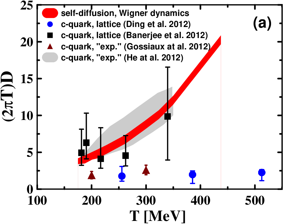
The self-diffusion constant and the viscosity-to-entropy ratio are presented in Fig. 8 as a function of temperature. The entropy density is taken from results of our PIMC calculations presented in Fig. 2. Our results are presented in the form of bands. The width of the bands represents the theoretical uncertainty associated with the oscillations of the antiderivative functions at large times, see Figs. 6 and 7. Slowly decaying oscillations of the time correlation functions are inherent in liquid-like systems of strongly interacting particles in contrast to exponentially decaying oscillations in gas-like systems. As known from hydrogen plasma, these oscillations arise because of quasiclosed chaotic orbits and are caused by strong interparticle interaction. In liquids these oscillations decay according to a power law rather than exponentially. Therefore, extremely long (in time) trajectories are required for more accurate calculations of the diffusion constant and viscosity. Due to CPU time limitations, we had to stop our computations before the decay of these oscillations was completed.
Unfortunately, the self-diffusion constant is unavailable from other calculations. Therefore, we compare it with heavy-quark diffusion constant, anticipating that these are of the same order of magnitude. The heavy-quark diffusion constant is available from recent QCD lattice computations [72, 59], which are presented in the Panel (a) of Figs. 8. Our results (labeled as “Wigner dynamics”) well agree with lattice data of Ref. [59], while essentially overestimate those of Ref. [72]. The heavy-quark diffusion constant is also available from analysis of experiments on heavy-quark quenching in ultrarelativistic heavy ions collisions at RHIC. For comparison we took two recent works on the subject [73, 74]. Here the results are also rather diverse. Estimates of Ref. [74] are well comparable with our result and lattice data of Ref. [59], while estimate of Ref. [73, 74] is considerably lower and better conforms to lattice results of Ref. [72].
Our results on the shear viscosity are presented in the Panel (b) of Figs. 8. As seen, the obtained values of viscosity are in the range of those deduced from the analysis of experimental elliptic flow in ultrarelativistic heavy ions collisions at RHIC, as summarized in Ref. [75]. Lattice data on the shear viscosity in the realistic case of the SU(3) group are not available, an extensive review of theoretical works on viscosity within QCD-motivated models is done in Ref. [76]. As seen, the minimum of the viscosity-to-entropy ratio is reached at a temperature above the expected phase transition rather than at the phase transition point, as is commonly expected. This minimum turns out to be quite shallow. The value of the viscosity-to-entropy ratio at the minimum is very close (from above) to the lower bound of for this quantity [77], often referred to as the KSS bound. With the temperature decrease, i.e. towards the hadronic phase, the viscosity rapidly rises.
V Conclusion
In this paper we demonstrated that color quantum Monte-Carlo (PIMC) simulations based on the quasiparticle model of the QGP are able to reproduce the lattice equation of state at zero baryon chemical potential at realistic model parameters (i.e. quasiparticle masses and coupling constant) even near the critical temperature and also yields valuable insight into the internal structure of the QGP. In our simulations we have introduced a new relativistic path integral measure and have developed a procedure of sampling color quasiparticle variables according to the SU(3) group Haar measure with appropriate Casimir conditions. Unfortunately, convergence of our calculations becomes poor in the range of the expected phase transition because the scheme suffers from jumps between stable and metastable states which turn out to be almost equally probable in this range. Our results indicate that the QGP reveals quantum liquid-like (rather than gas-like) properties up to the highest considered temperature of .
Short-distance correlations in the computed pair distribution functions of gluon-gluon and gluon-(anti)quark pairs displays the formation of clusters. In case of the gluon-gluon clusters we can even speak about gluon-gluon bound states, i.e. glueballs, at temperatures just above the phase transition. The possible existence of medium-modified meson-like bound states was actively discussed some time ago [67, 68]. Our result supports the conclusion of Ref. [71] on the absence of bound states above the temperature of the phase transition. This finding is in contrast to our previous results on the SU(2) group [29, 30, 31, 32]. There well pronounced bound states were found just above the critical temperature, which however quickly dissolved with the temperature rise. This happens because the SU(3) plasma turns out to be essentially denser than the SU(2) one, which is a consequence of a stronger effective attraction between the constituents. As a result, possible meson-like bound states in the SU(3) plasma just melt.
The PIMC method is not able to yield transport properties of the QGP. A way to access these is to develop a classical color molecular dynamics simulation [14], where quantum effects are included phenomenologically via a short-range potential. In contrast to these classical MD simulations [14], we have developed a more rigorous approach based on the combination of Feynman and Wigner formulations of quantum dynamics. The basic ideas of this approach have been briefly reported in Ref. [33]. In this paper we gave a more detailed description. In particular, this approach allowed us to calculate the self-diffusion coefficient and the viscosity of the strongly coupled QGP. Since the self-diffusion constant is unavailable from other calculations, we compared it with the heavy-quark diffusion constant, anticipating that these are of the same order of magnitude. The heavy-quark diffusion constant is available from recent QCD lattice computations [72, 59] and also from an analysis of the heavy-quark quenching in experiments on ultrarelativistic heavy ions collisions at RHIC. For comparison we took two recent works on such an analysis [73, 74]. Unfortunately the above mentioned lattice and heavy-quark-quenching results are rather diverse. Our self-diffusion constant well agrees with lattice data of Ref. [59] and estimates of Ref. [74], while essentially overestimates those of Refs. [72] and [72].
Our results on the shear viscosity are in the range of those deduced from the analysis of the experimental elliptic flow in ultrarelativistic heavy ions collisions at RHIC, as summarized in Ref. [75], i.e. in terms of the viscosity-to-entropy ratio, , in the temperature range from 170 to 440 MeV. The minimum of the viscosity-to-entropy ratio is reached at a temperature ( MeV), above the expected phase transition rather than at the phase transition point as commonly expected. This minimum turns out to be very shallow. The value of the viscosity-to-entropy ratio at the minimum is very close (from above) to the lower bound of for this quantity [77], i.e. to the KSS bound. With the temperature decrease, i.e. towards the hadronic phase, the viscosity rapidly rises.
Our present analysis is still confined only to the case of zero baryon chemical potential. Simulations at nonzero baryon chemical potentials are in progress.
We acknowledge stimulating discussions with P. Levai, D. Blaschke, R. Bock, H. Stoecker, and D.N.Voskresensky. Y.B.I. was partially supported by grant of the Russian Ministry of Science and Education NS-215.2012.2.
Appendix I: Integration over SU(3) group Haar measure
In this appendix we explain details of integration over SU(3) Haar measure in Eq. (7). The measure for single color charge in case of the SU(3) group is [9, 78, 79, 80]
| (118) |
with summation over and constants given in Table 1. For the SU(N) group the quadratic and cubic Casimirs are with for qluons and for quarks and antiquarks, for gluons and for quarks, for antiquarks has opposite sign. In fact, the normalization constant depends on and Casimirs.
For random sampling of the variable in Monte-Carlo integration in Eq. (7) we change to the related canonical Darboux variables for the SU(3) group. The set of the canonical variables is defined by the canonical Poisson bracket
| (119) |
where and are conventional coordinate and momentum, respectively, and obey
| (120) |
The color variables form a representation of SU(3). In terms canonical variables their Poison bracket reads
| (121) |
where are the structure constants of SU(3) given in Table 1.
| values |
|---|
| values |
|---|
The explicit transformations to canonical variables are given [9, 78, 79, 80] by expressions:
| (122) |
in which we have used definitions:
| (123) |
and and are given by
| (124) |
In this expression the set forms an SU(2) subgroup with quadratic Casimir . Let us note that two Casimirs depend only on and . They can be computed using the values given in Table 1 as
| (125) |
The phase space color measure for SU(3), given in Eq. (118) can be transformed to the new coordinates through use of Eq. (122) and evaluation of the Jacobian
| (126) |
Then the measure reads
| (127) | |||||
Since the two Casimirs are independent, the -functions fix both and . After integration over and the Eq. (127) gives a proper canonical volume element . Thus applying Metropolis algorithm to variables we can construct Markovian chain in phase space and obtain random color variables for calculation partition function according to the SU(3) group Haar measure with two Casimir conditions.
Appendix II: Lebesque-Dirac delta theorem
Let be a summable function of real argument such that .
Then when .
Proof: Let be any test function. Then
References
- [1] E. Shuryak, Prog. Part. Nucl. Phys. 62, 48 (2009) [arXiv:0807.3033 [hep-ph]]; ibid.53, 273 (2004) [arXiv:hep-ph/0312227].
- [2] J. Schukraft, arXiv:1112.0550 [arXiv:hep-ex].
- [3] C. Shen and U. Heinz, Phys. Rev. C 85, 054902 (2012) [arXiv:1202.6620 [nucl-th]].
- [4] Z. Fodor and S. D. Katz, arXiv:0908.3341 [hep-ph].
- [5] S. Borsanyi, G. Endrodi, Z. Fodor, A. Jakovac, S. D. Katz, S. Krieg, C. Ratti, K. K. Szabo, JHEP 1011, 077 (2010) [arXiv:1007.2580 [hep-lat]].
- [6] M. Cheng et al., Phys. Rev. D 81, 054504 (2010) [arXiv:0911.2215 [hep-lat]].
- [7] H. B. Meyer, Phys. Rev. D 76, 101701 (2007) [arXiv:0704.1801 [hep-lat]].
- [8] P. Hartmann, Z. Donko, P. Levai, G.J. Kalman, J. Phys. A42, 214029 (2006); Nucl. Phys. A774, 881-884, (2006) [arXiv:nucl-th/0601017].
- [9] D. F. Litim and C. Manuel, Phys. Rev. Lett. 82, 4981 (1999) [arXiv:hep-ph/9902430]; Nucl.Phys. B 562, 237 (1999) [arXiv:hep-ph/9906210]; Phys. Rev. D 61, 125004 (2000) [arXiv:hep-ph/9910348]; Phys. Rep. 364, 451 (2002) [arXiv:hep-ph/0110104].
- [10] M. Laine and C. Manuel, Phys. Rev. D 65, 077902 (2002) [arXiv:hep-ph/0111113].
- [11] C. Manuel and S. Mrowczynski, Phys. Rev. D 68, 094010 (2003) [arXiv:hep-ph/0306209].
- [12] P. F. Kelly, Q. Liu, C. Lucchesi and C. Manuel, Phys. Rev. D 50, 4209 (1994) [arXiv:hep-ph/9406285].
- [13] M. Hofmann, M. Bleicher, S. Scherer, et al., Phys. Lett. B 478, 161 (2000) [arXiv:nucl-th/9908030].
- [14] B.A. Gelman, E. V. Shuryak, and I. Zahed, Phys. Rev. C 74, 044908 (2006) [nucl-th/0601029]; ibid. 74, 044909 (2006) [arXiv:nucl-th/0605046].
- [15] S. Cho and I. Zahed, Phys. Rev. C 79, 044911 (2009) [arXiv:0812.1736 [nucl-th]]; ibid. 80, 014906 (2009) [arXiv:0812.1741 [nucl-th]]; ibid. 82, 054907 (2010) [arXiv:0910.2666 [nucl-th]]; ibid. 82, 064904 (2010) [arXiv:0910.1548 [nucl-th]]; ibid. 82, 044905 (2010) [arXiv:0909.4725 [nucl-th]]; K. Dusling and I. Zahed, Nucl. Phys. A 833, 172 (2010) [arXiv:0904.0169 [nucl-th]].
- [16] M.H. Thoma, IEEE Trans. Plasma Science 32, 738 (2004).
- [17] A. Filinov, M. Bonitz, and W. Ebeling, J. Phys. A 36, 5957 (2003).
- [18] G. Kelbg, Ann. Phys. (Leipzig) 12, 219 (1962); 13, 354 (1963).
- [19] K. Dusling and C. Young, arXiv:0707.2068 [nucl-th].
- [20] A. Filinov, V. Golubnychiy, M. Bonitz, et al., Phys. Rev. E 70, 046411 (2004).
- [21] M. Bonitz, A. Filinov, V. Golubnychyi, et al., J. Phys. A 36, 5921 (2003); Phys. 15, 055704 (2008).
- [22] V. S. Filinov, M. Bonitz, W. Ebeling, and V. E. Fortov, Plasma Phys. Control. Fusion 43, 743 (2001).
- [23] V. S. Filinov, M. Bonitz, and V. E. Fortov, JETP Lett. 72, 245 (2000).
- [24] M. Bonitz, V. S. Filinov, V. E. Fortov., et al., Phys. Rev. Lett. 95, 235006 (2005).
- [25] V. S. Filinov, M. Bonitz, P. R. Levashov, et al., J. Phys. A 36, 6069 (2003).
- [26] M. Bonitz, V. S. Filinov, V. E. Fortov, et al., J. Phys. A 39, 4717 (2006).
- [27] V. S. Filinov, H. Fehske, M. Bonitz, et al., Phys. Rev. E 75 , 036401 (2007).
- [28] V. S. Filinov, V. E. Fortov, P. R. Levashov, Y. B. Ivanov, M. Bonitz, V. E. Fortov and P. R. Levashov, Phys. Lett. A 376, 1096 (2012) [arXiv:1203.2191 [hep-ph]].
- [29] V. S. Filinov, M. Bonitz, Y. B. Ivanov, V. V. Skokov, P. R. Levashov and V. E. Fortov, Contrib. Plasma Phys. 52, 135 (2012).
- [30] V. S. Filinov, Y. B. Ivanov, M. Bonitz, P. R. Levashov and V. E. Fortov, Phys. Atom. Nucl. 74, 1364 (2011).
- [31] V. S. Filinov, Y. B. Ivanov, M. Bonitz, P. R. Levashov and V. E. Fortov, Phys. Atom. Nucl. 75, 693 (2012).
- [32] V. S. Filinov, M. Bonitz, Y. B. Ivanov, V. V. Skokov, P. R. Levashov and V. E. Fortov, Contrib. Plasma Phys. 49, 536 (2009) [arXiv:0905.0324 [nucl-th]].
- [33] V. S. Filinov, M. Bonitz, Y.B. Ivanov, V.V. Skokov, P.R. Levashov, and V.E. Fortov, Contrib. Plasma. Phys. 51, N4, 322-327 (2011).
- [34] P. Petreczky, F. Karsch, E. Laermann, S. Stickan, and I. Wetzorke, Nucl. Phys. Proc. Suppl. 106, 513 (2002) [arXiv:hep-lat/0110111].
- [35] J. Liao and E. V. Shuryak, Phys. Rev. D 73, 014509 (2006).
- [36] F. Karsch and M. Kitazawa, Phys. Rev. D 80, 056001 (2009) [arXiv:0906.3941 [hep-lat]].
- [37] S. K. Wong, Nuovo Cimento A 65, 689 (1970).
- [38] R. D. Pisarski, Phys. Rev. Lett. 63, 1129 (1989).
- [39] E. Braaten and R. D. Pisarski, Nucl. Phys. B337, 569 (1990); B339, 310 (1990).
- [40] J. Blaizot and E. Iancu, Phys. Rept. 359, 355 (2002) [arXiv:hep-ph/0101103].
- [41] E. E. Salpeter and H. A. Bethe, Phys. Rev. 84, 1232, (1951).
- [42] E. E. Salpeter, Phys. Rev. 87, 328, (1952).
- [43] W. Lucha, F. F. Schoberl, and D. Gromes, Phys. Rep. 200, 127, (1991).
- [44] W. Lucha, F. F. Schoberl, Int. J. Mod. Phys. A7, 6431, (1992).
- [45] R. P. Feynman, and A. R. Hibbs, Quantum Mechanics and Path Integrals (McGraw-Hill, New York, 1965).
- [46] V. M. Zamalin, G. E. Norman, and V. S. Filinov, The Monte-Carlo Method in Statistical Thermodynamics (Nauka, Moscow, 1977), (in Russian).
- [47] K. Huang,Statistical Mechanics (John Wiley&Sons, Inc., New York - London, 1963)
- [48] V. Tatarskii, Sov. Phys. Uspekhi 26, 311 (1983).
- [49] V. Filinov, Y. Medvedev, V. Kamskii, Mol. Phys. 85(4), 711 (1995).
- [50] G. Ciccotti, C. Pierleoni, F. Capuani, V. Filinov, Comp. Phys. Comm. 121-122, 452 (1999).
- [51] S. Cho and I. Zahed, Phys. Rev. C 82, 054907 (2010) [arXiv:0910.2666 [nucl-th]];
- [52] D.N. Zubarev, Nonequilibrium Statistical Thermodynamics, Plenum Press, New York/London 1974.
- [53] J.D. Doll, D.L. Freeman, T.L. Beck, Adv. Chem. Phys. 78, 61-127 (1990).
- [54] V.S. Filinov, J. Mol. Phys. 88, 1517, 1529 (1996).
- [55] V. Filinov, P. Thomas, I. Varga, T. Meier, M. Bonitz, V. Fortov and S. Koch, Phys. Rev. B65, 165124, (2002).
- [56] D. V. Shirkov and I. L. Solovtsov, Phys. Rev. Lett. 79 (1997) 1209; Nucl. Phys. Proc. Suppl. 64, 106 (1998).
- [57] G. M. Prosperi, M. Raciti, and C. Simolo, Prog. Part. Nucl. Phys. 58, 387 (2007) [arXiv:hep-ph/0607209].
- [58] O. Kaczmarek, F. Karsch, F. Zantow, and P. Petreczky, Phys. Rev. D 72, 059903 (2005) [arXiv:hep-lat/0406036].
- [59] D. Banerjee, S. Datta, R. Gavai and P. Majumdar, Phys. Rev. D 85, 014510 (2012) [arXiv:1109.5738 [hep-lat]].
- [60] A. Nakamura, T. Saito and S. Sakai, Phys. Rev. D 69, 014506 (2004) [arXiv:hep-lat/0311024].
- [61] A. Peshier, B. Kampfer, and O.P. Pavlenko, Phys. Rev. D 54, 2399 (1996).
- [62] Yu. B. Ivanov, V. V. Skokov, and V. D. Toneev, Phys. Rev. D 71, 014005 (2005) [arXiv:hep-ph/0410127].
- [63] A. V. Filinov, V. S. Filinov, Yu. E. Lozovik and M. Bonitz, Introduction to Computational Methods for Many-Body Physics, Ed. by M. Bonitz and D. Semkat (Rinton Press, Princeton, 2006).
- [64] V.S. Filinov, M. Bonitz, W. Ebeling, and V.E. Fortov, Plasma Physics and Controlled Fusion 43, 743-759 (2001).
- [65] V. Filinov, H. Fehske, M. Bonitz, V.E. Fortov, and P.R. Levashov, Phys. Rev. E75 , 036401 (2007).
- [66] V. I. Yukalov and E. P. Yukalova, Physica A 243, 382 (1997); Fiz. Elem. Chastits At. Yadra 28, 89 (1997).
- [67] E. V. Shuryak and I. Zahed, Phys. Rev. C 70, 021901 (2004) [arXiv:hep-ph/0307267]; Phys. Rev. D 70, 054507 (2004) [arXiv:hep-ph/0403127].
- [68] G. E. Brown, B. A. Gelman, and M. Rho, arXiv:nucl-th/0505037.
- [69] M. Asakawa, T. Hatsuda and Y. Nakahara, Prog. Part. Nucl. Phys. 46, 459 (2001) [arXiv:hep-lat/0011040]; Nucl. Phys. A 715, 863 (2003) [Nucl. Phys. Proc. Suppl. 119, 481 (2003)] [arXiv:hep-lat/0208059]; M. Asakawa and T. Hatsuda, Phys. Rev. Lett. 92, 012001 (2004) [arXiv:hep-lat/0308034].
- [70] S. Datta, F. Karsch, P. Petreczky and I. Wetzorke, Phys. Rev. D 69, 094507 (2004) [arXiv:hep-lat/0312037].
- [71] V. Koch, A. Majumder, and J. Randrup, Phys. Rev. Lett. 95, 182301 (2005) [arXiv:nucl-th/0505052].
- [72] H. T. Ding, A. Francis, O. Kaczmarek, F. Karsch, H. Satz and W. Soeldner, Phys. Rev. D 86, 014509 (2012) [arXiv:1204.4945 [hep-lat]].
- [73] P. Gossiaux, J. Aichelin and T. Gousset, Prog. Theor. Phys. Suppl. 193, 110 (2012) [arXiv:1201.4038 [hep-ph]]; P. B. Gossiaux, J. Aichelin, M. Bluhm, T. Gousset, M. Nahrgang, S. Vogel and K. Werner, PoS QNP 2012, 160 (2012) [arXiv:1207.5445 [hep-ph]].
- [74] M. He, R. J. Fries and R. Rapp, arXiv:1204.4442 [nucl-th].
- [75] S. A. Bass, Nucl. Phys. A 862-863, 174 (2011).
- [76] A. S. Khvorostukhin, V. D. Toneev and D. N. Voskresensky, Nucl. Phys. A 845, 106 (2010) [arXiv:1003.3531 [nucl-th]].
- [77] P. Kovtun, D. T. Son and A. O. Starinets, Phys. Rev. Lett. 94, 111601 (2005) [arXiv:hep-th/0405231].
- [78] K. Johnson, Ann. Phys. 192, 104, (1989).
- [79] P.F. Kelly, Q. Liu, C. Lucchesi and C. Manuel, Phys. Rev. Lett. 72, 3461, (1994).
- [80] P.F. Kelly, Q. Liu, C. Lucchesi and C. Manuel, Phys. Rev. D50, 4209, (1994).