Dispersive effects in the unitary Fermi gas
Abstract
We investigate within density functional theory various physical properties of the zero-temperature unitary Fermi gas which critically depend on the presence of a dispersive gradient term in the equation of state. First, we consider the unitary Fermi superfluid gas confined to a semi-infinite domain and calculate analytically its density profile and surface tension. Then we study the quadrupole modes of the superfluid system under harmonic confinement finding a reliable analytical formula for the oscillation frequency, which reduces to the familiar Thomas-Fermi one in the limit of a large number of atoms. Finally, we discuss the formation and propagation of dispersive shock waves in the collision between two resonant fermionic clouds, and compare our findings with recent experimental results.
PACS numbers: 05.30.Fk, 03.75.Ss, 67.85.-d
1 Introduction
In the last years the crossover from the weakly paired Bardeen-Cooper-Schrieffer (BCS) state to the Bose-Einstein condensate (BEC) of molecular dimers with ultra-cold two-hyperfine-components Fermi vapors atoms has been investigated by several experimental and theoretical groups 1. When the densities of the two spin components are equal, and when the gas is dilute so that the range of the inter-atomic potential is much smaller than the inter-particle distance, then the interaction effects are described by only one parameter: the s-wave scattering length, whose sign determines the character of the gas. Fano-Feshbach resonances can be used to change the value and the sign of the scattering length, simply by tuning an external magnetic field. At resonance the scattering length diverges so that the gas displays a very peculiar character, being at the same time dilute and strongly interacting. In this regime all scales associated with interactions disappear from the problem and the energy of the system is expected to be proportional to that of a non interacting fermions system. This is called the unitary regime 1, 2.
Recently it has been remarked 2 that the superfluid unitary Fermi gas, characterized by a divergent s-wave scattering length 1, can be efficiently described at zero temperature by phenomenological density functional theory. Indeed, different theoretical groups have proposed various density functionals. For example Bulgac and Yu have introduced a superfluid density functional based on a Bogoliubov-de Gennes approach to superfluid fermions 3, 4. Papenbrock and Bhattacharyya 5 have instead proposed a Kohn-Sham density functional with an effective mass to take into account nonlocality effects. Here we adopt instead the extended Thomas-Fermi functional of the unitary Fermi gas that we have proposed few years ago 6. The total energy in the extended Thomas-Fermi functional contains a term proportional to the kinetic energy of a uniform non interacting gas of fermions with number density , plus a gradient correction of the form , originally introduced by von Weizsäcker to treat surface effects in nuclei 7, and then extensively applied to study electrons 8, showing good agreement with Kohn-Sham calculations. In the context of the BCS-BEC crossover, the presence of the gradient term (and its actual weight) is a debated issue 9, 10, 11, 12, 13, 14, 15, 16. The main advantage of using such a functional is that, as it depends only on a single function of the coordinates, i.e. the order parameter, can be used to study systems with quite large number of particles . Other functionals, which are based instead on single-particle orbitals, require self-consistent calculations with a numerical load rapidly increasing with .
In the last years we have successfully applied our extended Thomas-Fermi density functional and its time-dependent version 6 to investigate density profiles 6, 17, collective excitations 17, Josephson effect 18 and shock waves 19, 20 of the unitary Fermi gas. In addition, the collective modes of our density functional have been used to study the low-temperature thermodynamics of the unitary Fermi gas (superfluid fraction, first sound and second sound) 21 and also the viscosity-entropy ratio of the unitary Fermi gas from zero-temperature elementary excitations 22.
For the superfluid unitary Fermi gas one expects the coexistence of dispersive and dissipative terms in the equation of state 20, 21, 22, 23. However, at zero temperature only dispersive term survive 20, 24. In this paper we investigate various physical quantities of the unitary Fermi gas, which depend on the presence of a dispersive gradient term in the zero-temperature equation of state. In the fist part we investigate static properties like density profiles and surface tension. In the second part we study dynamical properties like collective oscillations and dispersive shock waves due to the collision between two fermionic clouds.
2 Extended Thomas-Fermi density functional
The energy density of a uniform Fermi gas at unitarity depends on the constant density as follows 1
| (1) |
where is a universal parameter of the Fermi gas 1. In the presence of an external trapping potential the Hohenberg-Kohn theorem 25 ensures that the ground-state local density of the system can be obtained by minimizing the energy functional
| (2) |
where is a (generally unknown) energy functional of the internal energy, which is independent on . In our extended Thomas-Fermi approach we choose
| (3) |
where the local energy density is given by
| (4) |
In this expression, which is the equation of state (internal energy density) of the inhomogeneous system, the first term is the Thomas-Fermi-like term describing the uniform system, while the second term is the von Weizsäcker gradient correction 7. We have obtained the value by fitting accurate Monte Carlo results for the energy of fermions confined in a spherical harmonic trap close to unitary conditions 6, 26.
3 Semi-infinite domain: density profile and surface tension
We put in evidence the effects of the gradient term of our density functional by considering the external potential
| (5) |
acting on the Fermi superfluid. This implies that the superfluid density must go to zero at the boundary , while it becomes a constant far from the boundary. Since in the present calculations we fix the chemical potential rather than the total number of fermions , it is useful to introduce the zero-temperature grand potential energy functional of the unitary Fermi gas
| (6) |
It is convenient to introduce the characteristic length of the system
| (7) |
and to rewrite the density in terms of a function of the adimensional variable as
| (8) |
The grand-potential (6) then becomes:
| (9) |
where . is the area in the plane and is the length in the direction. The function minimizing the grand-potential obeys the equation:
| (10) |
with the boundary conditions The first integral of the system is
| (11) |
By using the appropriate boundary conditions we find and . It is then straightforward to get the integral equation
| (12) |
which gives implicitly the profile function .

In Fig. 1 we plot the scaled density profile obtained from the numerical integration (solid line) of Eq. (12), together with the function (dot-dashed line), which provides an excellent overall approximation to it.
In the limit the grand potential energy is divergent due to the asymptotic energy
| (13) |
where and . The surface tension is defined as
| (14) |
in the limit , i.e.
| (15) |
Eq. (11) with , and , helps us to rewrite the formula of the surface tension as
| (16) |
where .
In Fig. 2 we plot the surface tension as a function of the von Weizsäcker gradient coefficient setting 1, 6. By using , which is a reasonable estimate 6, 30 consistent with Monte Carlo results 6, 18, one finds This value is of the same order of magnitude of previous microscopic determinations of the surface tension based on different theoretical approaches27, 28, 29 and different boundary conditions at the interface.
4 Extended superfluid hydrodynamics

Let us now consider dynamical properties of the unitary Fermi gas. The starting point are the zero-temperature equations of superfluid hydrodynamics 24, given by
| (17) | |||
| (18) |
where where is the time-dependent scalar density field and is the time-dependent vector velocity field. In the case of the unitary Fermi gas the local energy density can be written by using Eq. (4). If , then Eqs. (17) and (18) reproduce by construction the familiar equations of superfluid hydrodynamics 1.
For a fermionic superfluid the velocity is irrotational, i.e. , and the circulation is quantized, i.e.
| (19) |
where is an integer quantum number. This means that the velocity field of the unitary Fermi gas can be written as
| (20) |
where is the phase of the Cooper pairs 1, 30. Eqs. (17) and (18) can be interpreted as the Euler-Lagrange equations of the following action functional
| (21) |
which depends on the local density and the phase . In the next section we use this action functional (21) to investigate zero-temperature collective oscillations of the unitary Fermi gas trapped by an external potential.
5 Quadrupole oscillations

In the case of spherically-symmetric harmonic confinement, i.e.
| (22) |
we have numerically studied 17 the collective modes of the unitary Fermi gas for different number of atoms by means of Eqs. (17) and (18). As predicted by Y. Castin 31, the frequency of the monopole mode (breathing mode) and the frequency dipole mode (center of mass oscillation) do not depend on :
| (23) |
We have found 17 instead that the frequency of the quadrupole () mode depends on and on the choice of the gradient coefficient . In particular, in Ref. 17 we have calculated for increasing values of up to .
In this paper we extend our previous calculations by taking into account much larger values of . To excite the quadrupole mode, we solve numerically Eqs. (17) and (18) with the initial condition
| (24) | |||||
| (25) |
where is the ground-state density profile and a small parameter. The results are shown in Fig. 3 where we plot the quadrupole frequency as a function of the number of atoms for three values of the gradient coefficient .
The numerical results of the figure can quite well be captured by a time-dependent Gaussian variational approach 32. We set
| (26) |
and
| (27) |
where , , , and are the time-dependent variational parameters. Inserting these quantities into the action functional (21), after integration over space variables we find
| (28) |
where the effective Lagrangian is given by
| (29) |
with . From this effective Lagrangian we calculate analytically the small oscillations around the equilibrium configuration, following the procedure described in Ref.32. In this way we get the following formula for the frequency of the quadrupole mode:
| (30) |
In the limit it gives the Thomas-Fermi result 1 , while in the limit it gives , which is the quadrupole oscillation frequency of non-interacting atoms 1. The curves reported in Fig. 3 show that this analytical formula reproduces remarkably well the numerical results (filled squares). This fact suggests the possibility of using Eq. (30) to determine the value of from experimental measurements of .
6 Collision of resonant Fermi clouds
We use here the generalized superfluid hydrodynamics equations to obtain the long-time dynamics of the collision between two initially separated Fermi clouds, simulating the experiments of Ref. 33. The details of our calculations can be found in Ref. 20. Here we summarize the main results of our study. In our simulations we tried to reproduce as closely as possible the experimental conditions of Ref. 33 which we summarize briefly in the following. A 50:50 mixture of the two lowest hyperfine states of 6Li (for a total of atoms) is confined by an axially symmetric cigar-shaped laser trap, elongated along the z-axis. The resulting trapping potential is , where , Hz and Hz. The trapped Fermi cloud is initially bisected by a blue-detuned beam which provides a repulsive knife-shaped potential. This potential is then suddenly removed, allowing for the two separated parts of the cloud to collide with each other. The system is then let to evolve for a given hold time after which the trap in the radial direction is removed. The system is allowed to evolve for another ms during which the gas expands in the r-direction (during this extra expansion time, the confining trap frequency along the z-axis is changed to Hz), and finally a (destructive) image of the cloud is taken. The process is repeated from the beginning for another different value for the hold time . The main effect observed in the experiment 33 is the presence of shock waves, i.e. of regions characterized by large density gradients, in the colliding clouds. The experimental results are shown in the right part of Fig. 4 as a sequence of one-dimensional profiles obtained by averaging along one transverse direction the observed cloud density at different times.

We simulated the whole procedure by using the Runge-Kutta-Gill fourth-order method 34, 35 to propagate in time the solutions of the following non-linear Schrödinger equation (NLSE)
| (31) |
which is strictly equivalent 6, 30 to Eqs. (17) and (18), with given by Eq. (4), and
| (32) |
Since the confining potential used in the experiments is cigar-shaped, we have exploited the resulting cylindrical symmetry of the system by representing the solution of our NLSE on a 2-dimensional grid. During the time evolution of our system, when the two clouds start to overlap, many ripples whose wavelength is comparable to the interparticle distance are produced in the region of overlapping densities. In order to properly compare our results with the experimental data of resonant fermions 33, which are characterized by a finite spatial resolution, we smooth the calculated profiles at each time by local averaging the density within a space window of centered around the calculated point.
The results of our simulations, for the whole time duration of the experiments, and after the smoothing procedure is applied to the (y-averaged) density profile at each time, are shown in the left part of Fig. 4 (see also Ref.20), plotted along the long trap axis, for the same time frames as in the experiment. Remarkably, there is a striking correspondence between the experimental data and the results of our simulation. At variance with the current interpretation of the experiments, where the role of viscosity is emphasized33, we obtained a quantitative agreement with the experimental observation of the dynamics of the cloud collisions within our superfluid effective hydrodynamics approach, where density variations during the collision are controlled by a purely dispersive quantum gradient term.
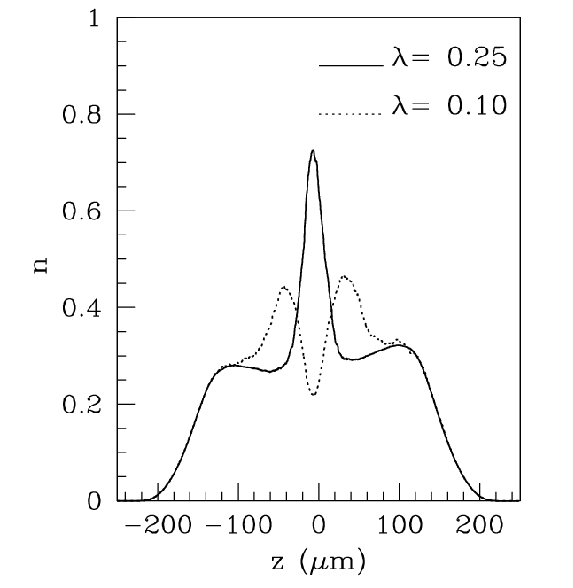
We find that changing from the optimal value has profound consequencies on the long-time evolution of the colliding clouds, providing density profiles which are completely different from the experimental ones. This is shown in Fig.5, where the simulated density profile after 3 ms is calculated using two different values for . Such a strong dependence on of the time evolution of a Fermi cloud made of a large number of atoms is at first sight surprising, because the gradient term should become less and less important with increasing . We believe that such dependence is due to the presence of shock waves (i.e. regions characterized by large density gradients) in the colliding clouds, as discussed in Ref.20.
7 Conclusions
In the first part of the paper we have calculated the density profile and surface tension of the superfluid unitary Fermi gas in a semi-infinite domain by using the extended Thomas-Fermi density functional, where the surface effects are modelled by the the von Weizsäcker gradient term. Indeed we have found that is proportional to , where is the phenomenological coefficient of the von Weizsäcker term. In the second part of the paper we have investigated dispersive dynamical effect which crucially depend on the presence of a gradient term in the equation of state of the unitary Fermi gas. In particular, we have studied the quadrupole modes of the superfluid system under harmonic confinement, finding a reliable analytical formula for the oscillation frequency, which reduces to the familiar Thomas-Fermi one in the limit of a large number of atoms. Finally, we have numerically studied the long-time dynamics of shock waves in the ultracold unitary Fermi gas. Two main results emerge from our calculations: a) at zero temperature the simplest regularization process of the shock is purely dispersive, mediated by the quantum gradient term, which is one of the ingredient in our DF approach; b) the quantum gradient term plays an important role not only in determining the static density profile of small systems, where surface effects are important, but also in the fast dynamics of large systems, where large density gradients may arise.
Acknowledgements.
We thank James Joseph, John E. Thomas and Manas Kulkarni for fruitful discussions.References
- 1 W. Zwerger (ed.), BCS-BEC Crossover and the Unitary Fermi Gas, Lecture Notes in Physics, vol. 836 (Springer, Berlin, 2011).
- 2 A. Bulgac, M. Mc Neil Forbes, and P. Magierski, in BCS-BEC Crossover and the Unitary Fermi Gas, Lecture Notes in Physics, vol. 836, Ed. by W. Zwerger (Springer, Berlin, 2011).
- 3 A. Bulgac and Y. Yu, Phys. Rev. Lett. 91, 190404 (2003).
- 4 A. Bulgac, Phys. Rev. A 76, 040502(R) (2007).
- 5 T. Papenbrock, Phys. Rev. A 72, 041603(R) (2005); A. Bhattacharyya and T. Papenbrock, Phys. Rev. A 74, 041602(R) (2006).
- 6 L. Salasnich and F. Toigo, Phys. Rev. A 78, 053626 (2008); L. Salasnich and F. Toigo, Phys. Rev. A 82, 059902(E) (2010).
- 7 C.F. von Weizsäcker, Zeit. Phys. 96, 431 (1935).
- 8 D. A. Kirzhnits, Zh. Eksp. Teor. Fiz. 32, 115 (1957) [Sov. Phys. JETP 5, 64 (1957)]; C.H. Hodges, Can. J. Phys. 51, 1428 (1973). E. Zaremba and H.C. Tso, Phys. Rev. B 49, 8147 (1994); Z. Yan, J. P. Perdew, T. Korhonen, and P. Ziesche, Phys. Rev. A 55, 4601 (1997).
- 9 Y.E. Kim and A.L. Zubarev, Phys. Rev. A 70, 033612 (2004).
- 10 M.A. Escobedo, M. Mannarelli and C. Manuel, Phys. Rev. A 79, 063623 (2009).
- 11 E. Lundh and A. Cetoli, Phys. Rev. A 80, 023610 (2009).
- 12 G. Rupak and T. Schäfer, Nucl. Phys. A 816, 52 (2009).
- 13 S.K. Adhikari, Laser Phys. Lett. 6, 901 (2009).
- 14 W.Y. Zhang, L. Zhou, and Y.L. Ma, EPL 88, 40001 (2009).
- 15 A. Csordas, O. Almasy, and P. Szepfalusy, Phys. Rev. A 82, 063609 (2010).
- 16 S. N. Klimin, J. Tempere, and J.P.A. Devreese, J. Low Temp. Phys. 165, 261 (2011).
- 17 L. Salasnich, F. Ancilotto, and F. Toigo, Laser Phys. Lett. 7, 78 (2010).
- 18 F. Ancilotto, L. Salasnich, and F. Toigo, Phys. Rev. A 79, 033627 (2009).
- 19 L. Salasnich, EPL 96, 40007 (2011).
- 20 F. Ancilotto, L. Salasnich, and F. Toigo, Phys. Rev. A 85, 063612 (2012).
- 21 L. Salasnich, Phys. Rev. A 82, 063619 (2010).
- 22 L. Salasnich and F. Toigo, J. Low Temp. Phys. 165, 239 (2011).
- 23 M. Kulkarni and A.G. Abanov, e-preprint arXiv:1205.5917.
- 24 L.D. Landau and E.M. Lifshitz, Fluid Mechanics (Pergamon Press, London, 1987).
- 25 P. Hohenberg and W. Kohn, Phys. Rev. 136 B864 (1964).
- 26 S.K. Adhikari and L. Salasnich, New J. Phys. 11, 023011 (2009); S.K. Adhikari, J. Phys B 43, 085304 (2010).
- 27 H. Caldas, J. Stat. Mech. P11012 (2007).
- 28 S.K. Baur, Sourish Basu, T.N. De Silva and E.J. Mueller, Phys. Rev. A 79, 063628 (2009).
- 29 A. Kryjevski, Phys. Rev. A 78, 043610 (2008).
- 30 S.K. Adhikari and L. Salasnich, Phys. Rev. A 78 043616 (2008); L. Salasnich, Laser Phys. 19, 642 (2009).
- 31 Y. Castin, Comptes Rendus Physique 5, 407 (2004).
- 32 L. Salasnich, Int. J. Mod. Phys. B 14, 1 (2000).
- 33 J. Joseph, J. Thomas, M. Kulkarni, and A. Abanov, Phys. Rev. Lett. 106, 150401 (2011).
- 34 Mathematical Methods for Digital Computers, Ed. by A. Ralston and H. S. Wilf, vol. 1, p. 117 (Wiley, New York, 1960).
- 35 M. Pi, F. Ancilotto, E. Lipparini and R. Mayol, Physica E 24, 297 (2004).