Roughly speaking, the measurement problem consists in the fact that the Schrödinger equation of quantum mechanics generically fails to predict that measurements have outcomes. Instead, it apparently predicts (empirically) unacceptable “superpositions” thereof. Slightly more technically, the problem is usually formulated in approximately the following way (see e.g. the excellent presentations in [2, 18, 19] for more detail). Suppose that one measures some observable $O$ pertaining to a microscopic system $S$, in such a way that if $S$ is in an eigenstate $\Phi_{i}$ of $O$, then the associated macroscopic apparatus $A$ is in state $\Omega_{i}$. It is important to note that in this description (pure) states are seen as unit vectors in some Hilbert space, as usual in quantum mechanics. Now, although there is hardly any problem with the existence of a microscopic superposition $\Phi=\sum_{i}c_{i}\Phi_{i}$ of $S$ (where $\sum_{i}|c_{i}|^{2}=1$), the linearity of the Schrödinger equation implies that it would bring $S+A$ into a similar superposition $\Psi=\sum_{i}c_{i}\Psi_{i}$, $\Psi_{i}\equiv\Phi_{i}\otimes\Omega_{i}$, which, if macroscopic,⁵⁵ 5 This notion needs to be quantified, of course [2, 19]. See also [75] and the present paper. is never seen in nature. Instead, as a matter of fact one always observes one of the states $\Omega_{i}$ (or so it is claimed).

This problem was immediately recognized by the founders of quantum theory. In response, in 1926, Born (generalizing earlier ideas of Bohr and Einstein on light emission by atoms) stated that quantum theory indeed did not predict individual outcomes, but merely computed their probabilities (according to the formula now named after him) [14, 78]. In 1927, Heisenberg (again in the wake of Bohr’s electronic “quantum jumps”) proposed the “collapse of the wave-packet” [57], which (in the above language) implies that during the course of the measurement, the state $\Psi$ miraculously “jumps” to one of the states $\Psi_{i}$. Bohr immediately endorsed this idea, ordered that such quantum jumps ought not to be analyzed any further, and claimed that they were the source of irreducible randomness in physics. During the period 1927–1935 (with an aftermath running until 1949), Bohr famously defended these ideas against a highly critical Einstein [10], as did Born [13]. Adding considerable conceptual and mathematical precision, von Neumann gave an account of the measurement problem in his book from 1932 [89], which has formed the basis for most discussions of the issue ever since. The early period was closed in 1935, the year in which Schrödinger (following a correspondence with Einstein [43]) published a penetrating analysis, including the metaphor around the cat later named after him [103].

The introduction of the collapse process (and the associated Born probabilities) has turned out to be an incredibly successful move, on which practically all empirical successes of quantum theory are based. This may well be the reason why few physicists are bothered by the measurement problem: the underlying slick manoeuvre of ad hoc collapse seems an acceptable price for these successes, unprecedented in science as they are. But for those in the foundations of physics, there is no doubt that this is a pseudo-solution. Consequently, despite arguments claiming to prove their non-existence [16, 19, 42], many solutions to the measurement problem have been proposed. Among those, it is fair to say that at least the quasi-philosophical solutions have failed to convince the scientific community at large.⁶⁶ 6 This is true in particular for the Many-Worlds (aka “Everett”) Interpretation [100], or the Modal Interpretation of quantum mechanics [36], in which radical changes are proposed in the ontology and/or the usual interpretative rules of the theory, without clarifying in any way what is really going on during measurements (a question one indeed is not supposed to ask, according to received wisdom). Bohmian mechanics (as a modern incarnation of de Broglie’s pilot-wave theory) does a better job here [33, 38, 39], but its narrow applicability (at least in its current form), focusing as it does on position as the only physical observable, makes it unattractive to many (including the authors). See some kinship in §5.4, however.

Within the realm of technical approaches to the measurement problem, one may distinguish between those proposals that do and those that do not modify quantum theory. Among the latter, the main effort so far has been towards attempts to eliminate interference terms (i.e., between states like the $\Psi_{i}$ above), sometimes accompanied by the (implicit or explicit) suggestion that their removal would actually solve the problem.⁷⁷ 7 This applies, for example, to the famous paper by Danieri, Loinger, and Prosperi [34], to early papers on decoherence [117], and to much of the mathematical physics literature on the measurement problem, including the work of the senior author [40, 60, 72, 73, 108]. We now regard such papers as mathematically interesting but conceptually misguided, at least on this point. On the other hand, it is to the credit of especially the Swiss school that it drew attention to the idea that measurement involves limiting procedures, so that solutions of the measurement problem should at least incorporate the appropriate limits.

Such attempts come in (at least) two kinds. In the wake of the Swiss school [40, 60], mathematical physicists typically use the formalism of superselection rules (see [72, 73] for reviews and [108] for recent work in this direction), whereas theoretical physicists tend to exploit decoherence (see [68, 102] for recent reviews). There seems to be a general consensus, though, that neither of these solves the problem (at least in the form stated above); they rather reconfirm it. Indeed, granted that measurements yield classical data, since classical physics by definition does not have quantum-mechanical interference terms, their disappearance in appropriate limiting situations (like the ones described by decoherence and/or superselection theory) is just a necessary condition that (in part) defines measurement (which after all is supposed to produce some classical state as its outcome).⁸⁸ 8 In this sense even von Neumann’s book [89] is misleading, since he suggested that the act of observation may be identified with a cut in the chain now named after him. What is right about this idea is that observation is linked to a voluntary change of information, but it would have been preferable to point out that such a change, in so far as it defines measurement, should be a loss of quantum information. Consequently, in our opinion the measurement problem is posed, rather than solved by proving that such interference terms vanish under particular (limiting) conditions.⁹⁹ 9 Furthermore, despite its outspoken ambition to derive classical physics from quantum theory [68, 102, 117], decoherence hardly (if at all) invokes limits like Planck’s constant going to zero, which are needed, for one thing, to derive the correct classical equations of motion (cf. [75, 76]).

In contrast, the dynamical collapse models of Pearle, Ghirardi–Rimini–Weber, and others (cf. [2] for a comprehensive survey) do solve the measurement problem. But they do so at a price: the Schrödinger equation is modified by adding a novel and universal stochastic process that even makes the equation nonlinear, and which, like the solution of Heisenberg and von Neumann, is ad hoc except for its goal of causing collapse.

The approach to the measurement problem we are going to propose below uses key ideas from both dynamical collapse models and decoherence (and could not have been conceived without the inspiration from these earlier approaches), but in such a way that we avoid some of their drawbacks (though only in the context of a simple example, so far):

1. 1.

   Dynamical collapse is obtained without modifying quantum theory.

2. 2.

   While decoherence preserves all peaks (i.e., potential measurement outcomes) in the density matrix, and hence subsequently needs e.g. some kind of a Many Worlds Interpretation [63, 102, 113], our mechanism, if correct, leads to just one outcome.

Our approach starts with a technical reformulation of the measurement problem, which relies on a specific mathematical formalism for dealing with classical states, including their role as potential limits of quantum states. For completeness’ sake, we explain this first.

In order to describe classical states as limits of quantum states, we need to describe all states algebraically.¹⁰¹⁰ 10 An introduction for philosophers to the material in this section may be found in [75, Ch. 4&5]. Although this formalism implicitly uses the language of C*-algebras, very little of that theory will be needed here [53, 74]. The main point is to have a unified formalism for classical and quantum physics, from which the usual treatment in which classical physics is described using phase spaces having the structure of (differentiable) manifolds, whilst quantum physics is based on Hilbert spaces and operators, is a far cry.

Nonetheless, the necessary unification of these diverse instances of mathematical formalism may be achieved by focusing on the interplay between observables (or propositions) and states (as opposed to the reification of the notion of a state inherent in the usual approach, which is particularly detrimental to the measurement problem). Indeed, classical and quantum physics turn out to share the following mathematical structure:

• •

  The observables comprise the (self-adjoint part of) a C*-algebra $A$.¹¹¹¹ 11 A C*-algebra is a complex algebra $A$ that is complete in a norm $\|\cdot\|$ satisfying $\|ab\|\,\leq\,\|a\|\,\|b\|$ for all $a,b\in A$, and has an involution $a\rightarrow a^{*}$ such that $\|a^{*}a\|=\|a\|^{2}$.

• •

  The states are positive linear functionals $\omega:A\rightarrow{\mathbb{C}}$ of norm one on $A$.¹²¹² 12 Positivity of $\omega$ means that $\omega(a^{*}a)\geq 0$ for all $a\in A$. If $A$ has a unit $1$, then a state may equivalently be defined as a positive linear functional $\omega:A\rightarrow{\mathbb{C}}$ that satisfies $\omega(1)=1$.

• •

  A pure state $\omega$ has no nontrivial convex decomposition, i.e., if $\omega=p\omega_{1}+(1-p)\omega_{2}$ for some $p\in(0,1)$ and certain states $\omega_{1}$ and $\omega_{2}$, then $\omega_{1}=\omega_{2}=\omega$.

In the main example of interest for this paper, which is a particle moving on the real line, this abstract talk has a simple implementation (which suffices for what follows). Its main feature is that, as Heisenberg had it, the difference between the classical and the quantum setting lies in the non-commutativity of the observables in the latter (see also [25]).

Classical:

The C*-algebra of observables is $A_{0}=C_{0}({\mathbb{R}}^{2})$, that is, the continuous functions on the phase space ${\mathbb{R}}^{2}$ that vanish at infinity. The algebraic operations are defined pointwise (e.g., $(fg)(z)=f(z)g(z)$), involution is (pointwise) complex conjugation, and the norm is the supremum-norm. Hence $A_{0}$ is commutative. A state $\mu:A_{0}\rightarrow{\mathbb{C}}$ is essentially the same thing as a probability measure $\hat{\mu}$ on phase space through

$$\mu(f)=\int_{{\mathbb{R}}^{2}}d\hat{\mu}\,f.$$

(2.1)

Such a probability measure may or may not be given by a probability density with respect to the Liouville measure $dpdq/2\pi$, i.e., a positive $L^{1}$-function $\chi$ on ${\mathbb{R}}^{2}$ s.t.

$$\int_{{\mathbb{R}}^{2n}}\frac{dpdq}{2\pi}\,\chi(p,q)f(p,q)=\int_{{\mathbb{R}}^{2}}d\hat{\mu}\,f.$$

(2.2)

This also implies that $\chi$ integrates to unity (with respect to the Liouville measure). Pure states on $C_{0}({\mathbb{R}}^{2})$ are probability measures of the Dirac form $\delta_{z}$, $z\in{\mathbb{R}}^{2}$, i.e., $\delta_{z}(f)=f(z)$ for $f\in C_{0}({\mathbb{R}}^{2})$, and hence bijectively correspond to points of ${\mathbb{R}}^{2}$. Such states are not given by probability densities, however, as $\delta$-functions are not in $L^{1}$.

Quantum:

The C*-algebra of observables is $A=K(L^{2}({\mathbb{R}}))$ i.e., the algebra of compact operators on the Hilbert space $L^{2}({\mathbb{R}})$ of square-integrable wave-functions.¹³¹³ 13 A self-adjoint operator $a$ on a Hilbert space is compact just in case it has a spectral decomposition $a=\sum_{i}\lambda_{i}|e_{i}\rangle\langle e_{i}|$ (where $|e_{i}\rangle\langle e_{i}|$ is the orthogonal projection onto the ray ${\mathbb{C}}e_{i}$), where the eigenvectors $(e_{i})$ form an orthonormal basis of $H$, each nonzero eigenvalue $\lambda_{i}$ has finite multiplicity, and if the eigenvalues are listed in decreasing order of their absolute value (i.e., $\|a\|=|\lambda_{1}|\geq|\lambda_{2}|\geq\cdots$), then $\lim_{\alpha\rightarrow\infty}|\lambda_{\alpha}|=0$. Such operators may be added and multiplied in the obvious way; involution is hermitian conjugation, and the norm is the usual operator norm. States $\rho:K(L^{2}({\mathbb{R}}))\rightarrow{\mathbb{C}}$ bijectively correspond to density matrices $\hat{\rho}$ on $L^{2}({\mathbb{R}})$ through $\rho(a)=\mbox{\rm Tr}\,(\hat{\rho}a)$. A unit vector $\Psi$ defines a density matrix $|\Psi\rangle\langle\Psi|$, so that pure states $\psi$ on $K(L^{2}({\mathbb{R}}))$ bijectively correspond to unit vectors $\Psi$ up to a phase (or to rays ${\mathbb{C}}\cdot\Psi$) through

$$\psi(a)=\langle\Psi|a|\Psi\rangle\equiv\langle\Psi,a\Psi\rangle.$$

(2.3)

In both cases, an idealized description has been used in order to avoid unnecessary mathematical complications: first, inherently to the C*-algebraic formalism, one works with bounded operators (in quantum theory) and functions (classically).¹⁴¹⁴ 14 Although unbounded operators play a major practical role in physics (think of position and momentum), they may be awkward to deal with due to domain issues and in any case they can theoretically be avoided without any loss of generality. Indeed, unbounded self-adjoint operators $a$ bijectively correspond to bounded operators (or constructions involving those) in at least four different ways [96]. First, one may pass to the unitary Cayley transform $(a-i)(a+i)^{-1}$. Second, one may construct the associated one-parameter unitary group $t\mapsto\exp(ita)$ by Stone’s Theorem. Third, one may work with the bounded spectral projections, from which the operator may be reconstructed by the spectral theorem. Fourth, one could take the resolvents $(a-\lambda)^{-1}$, $\lambda\notin{\mathbb{R}}$ (whose typical integral kernels are Green’s functions). Second, the restriction to functions vanishing at infinity and compact operators in the classical and the quantum case, respectively, is also purely a matter of mathematical convenience.¹⁵¹⁵ 15 Classically, one could work with the (essentially) bounded integrable functions $L^{\infty}({\mathbb{R}}^{2})$, whilst in quantum theory one could take the algebra $B(L^{2}({\mathbb{R}}))$ of all bounded operators on $L^{2}({\mathbb{R}})$ (as opposed to merely the compact ones). These broader classes can be constructed from the $C_{0}$-functions or compact operators by taking pointwise and weak (or strong) limits, respectively. Enlarging the class of observables like that also brings in new continuity conditions on the states (namely $\sigma$-additivity and $\sigma$-weak continuity, respectively). Imposing these leads to the same states as discussed above; without them, one obtains more.

The following notion of convergence of quantum states to classical ones is standard (cf. [27, 74, 95, 98] and many other sources),¹⁶¹⁶ 16 Often Weyl quantization $Q^{W}_{\hbar}$ is used instead of Berezin quantization $Q_{\hbar}$, as in [9], but for Schwartz functions $f$ on phase space these have the same asymptotic properties as $\hbar\rightarrow 0$ [74]. The advantage of Berezin quantization is that it is well defined also for continuous functions vanishing at infinity, in that for any unit vector $\Psi\in L^{2}({\mathbb{R}})$ the map $f\mapsto\langle\Psi|Q_{\hbar}(f)|\Psi\rangle$ defines a probability measure on phase space. In contrast, the Wigner function defined by $f\mapsto\langle\Psi|Q^{W}_{\hbar}(f)|\Psi\rangle$ may fail to be positive, as is well known. and has been used especially in quantum chaology [91]. We first recall the coherent states, labeled by $z=(p,q)\in{\mathbb{R}}^{2}$,

$$\Phi^{(p,q)}_{\hbar}(x)=(\pi\hbar)^{-1/4}e^{-ipq/2\hbar}e^{ipx/\hbar}e^{-(x-q)^{2}/2\hbar},$$

(2.4)

with associated Berezin quantization map $f\mapsto Q_{\hbar}(f)$, $f\in C_{0}({\mathbb{R}}^{2})$, $Q_{\hbar}(f)\in K(L^{2}({\mathbb{R}}))$,

$$Q_{\hbar}(f)=\int_{{\mathbb{R}}^{2n}}\frac{dpdq}{2\pi\hbar}\,f(p,q)|\Phi^{(p,q)}_{\hbar}\rangle\langle\Phi^{(p,q)}_{\hbar}|.$$

(2.5)

Now let $(\rho_{\hbar})$ be a family of quantum states, indexed by $\hbar$ (say $\hbar\in(0,1]$), with associated density matrices $(\hat{\rho}_{\hbar})$, and let $\rho_{0}$ be a state on $C_{0}({\mathbb{R}}^{2})$, with associated probability measure $\hat{\rho}_{0}$ on ${\mathbb{R}}^{2}$. The quantum states $(\rho_{\hbar})$ converge to the classical state $\rho_{0}$ if for all $f\in C_{0}({\mathbb{R}}^{2})$,

$$\lim_{\hbar\rightarrow 0}\rho_{\hbar}(Q_{\hbar}(f))=\rho_{0}(f).$$

(2.6)

In that case we write $\lim_{\hbar\rightarrow 0}\rho_{\hbar}=\rho_{0}$. The condition (2.6) more explicitly reads

$$\lim_{\hbar\rightarrow 0}\mbox{\rm Tr}\,(\hat{\rho}_{\hbar}Q_{\hbar}(f))=\int_{{\mathbb{R}}^{2}}d\hat{\rho}_{0}\,f,\>\mbox{ for all }f\in C_{0}({\mathbb{R}}^{2}).$$

(2.7)

If $\rho_{\hbar}=|\Psi_{\hbar}\rangle\langle\Psi_{\hbar}|$, then obviously

$$\langle\Psi_{\hbar}|Q_{\hbar}(f)|\Psi_{\hbar}\rangle=\int_{{\mathbb{R}}^{2n}}\frac{dpdq}{2\pi\hbar}\,\chi_{\Psi_{\hbar}}(p,q)f(p,q),$$

(2.8)

where the probability density $\chi_{\Psi_{\hbar}}$, called the Husumi function of $\Psi_{\hbar}$, is given by

$$\chi_{\Psi_{\hbar}}(p,q)=|\langle\Phi^{(p,q)}_{\hbar}|\Psi_{\hbar}\rangle|^{2},$$

(2.9)

in which the inner product is taken in $L^{2}({\mathbb{R}})$. Consequently, if the limit in (2.6) exists for specific $\rho_{\hbar}=|\Psi_{\hbar}\rangle\langle\Psi_{\hbar}|$, then the limit measure $\hat{\rho}_{0}$ is the weak (or pointwise) limit of the probability measures $\mu_{\Psi_{\hbar}}$ defined by the probability densities $\chi_{\Psi_{\hbar}}$ according to (2.2).

Let us illustrate this formalism for the ground state of the one-dimensional harmonic oscillator. Taking $V(x)=\mbox{\footnotesize$\frac{1}{2}$}\omega^{2}x^{2}$ in the usual quantum Hamiltonian (with mass $m=1/2$),

$$H_{\hbar}=-\hbar^{2}\frac{d^{2}}{dx^{2}}+V(x),$$

(2.10)

it is well known that the ground state is unique and that its wave-function

$$\Psi_{\hbar}^{(0)}(x)=\left(\frac{\omega}{2\pi\hbar}\right)^{1/4}e^{-\omega x^{2}/4\hbar}$$

(2.11)

is a Gaussian, peaked above $x=0$. As $\hbar\rightarrow 0$, this ground state converges to the ground state $\rho_{0}^{(0)}=(0,0)\in{\mathbb{R}}^{2}$ (i.e., $(p=0,q=0)$) of the corresponding classical system. Slightly less familiar, the same is true for the anharmonic oscillator (with small $\lambda>0$), i.e.,

$$V(x)=\mbox{\footnotesize$\frac{1}{2}$}\omega^{2}x^{2}+\mbox{\footnotesize$\frac{1}{4}$}\lambda x^{4},$$

(2.12)

the peak, of course, now being only approximately Gaussian. But it is a deep and counterintuitive feature of quantum theory that even the symmetric double-well potential

$$V(x)=-\mbox{\footnotesize$\frac{1}{2}$}\omega^{2}x^{2}+\mbox{\footnotesize$\frac{1}{4}$}\lambda x^{4}+\mbox{\footnotesize$\frac{1}{4}$}\omega^{4}/\lambda=\mbox{\footnotesize$\frac{1}{4}$}\lambda(x^{2}-a^{2})^{2},$$

(2.13)

where $a=\omega/\sqrt{\lambda}>0$ (assuming $\omega>0$ as well as $\lambda>0$), has a unique quantum-mechanical ground state [62, 97], despite the fact that the corresponding classical system has two degenerate ground states, given by the phase space points $\rho_{0}^{\pm}\in{\mathbb{R}}^{2}$ defined by

$$\rho_{0}^{\pm}=(p=0,q=\pm a).$$

(2.14)

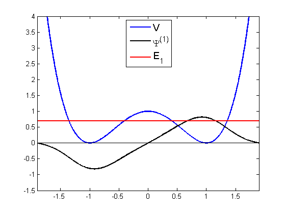
This ground state wave-function $\Psi_{\hbar}^{(0)}$ is again real and positive definite, but this time it has two peaks, above $x=\pm a$, with exponential decay $|\Psi_{\hbar}^{(0)}(x)|\sim\exp(-1/\hbar)$ in the classically forbidden region [62, 97]. As a quantum-mechanical shadow of the classical degeneracy, energy eigenfunctions (and the associated eigenvalues) come in pairs. In what follows, we will be especially interested in the first excited state $\Psi_{\hbar}^{(1)}$, which like $\Psi^{(0)}_{\hbar}$ is real, but has one peak above $x=a$ and another peak below $x=-a$. See Figure 1.

As $\hbar\rightarrow 0$, the eigenvalue splitting $E_{1}-E_{0}$ vanishes exponentially in $-1/\hbar$ like

$$\Delta\equiv E_{1}-E_{0}\sim(\hbar\omega/\sqrt{\mbox{\footnotesize$\frac{1}{2}$}e\pi})\cdot e^{-d_{V}/\hbar}\>\>(\hbar\rightarrow 0),$$

(2.15)

where the typical wkb-factor is given by

$$d_{V}=\int_{-a}^{a}dx\,\sqrt{V(x)};$$

(2.16)

see [46, 71] (heuristic), or [58, 62, 110] (rigorous) for details. Also, the probability density of each of the wave-functions $\Psi^{(0)}_{\hbar}$ or $\Psi_{\hbar}^{(1)}$ contains approximate $\delta$-function peaks above both classical minima $\pm a$. See Figure 2, displayed just for $\Psi^{(0)}_{\hbar}$, the other being analogous.

We can make the correspondence between the nondegenerate pair $(\Psi^{(0)}_{\hbar},\,\Psi_{\hbar}^{(1)})$ of low-lying quantum-mechanical wave-functions and the pair $(\rho_{0}^{+},\rho_{0}^{-})$ of degenerate classical ground states more transparent by invoking the above notion of a classical limit. Indeed, in terms of the corresponding algebraic states $\psi^{(0)}_{\hbar}$ and $\psi_{\hbar}^{(1)}$, cf. (2.3), one has

	$\displaystyle{\lim_{\hbar\rightarrow 0}\psi_{\hbar}^{(0)}}$	$\displaystyle=$	$\displaystyle\lim_{\hbar\rightarrow 0}\psi^{(1)}_{\hbar}=\rho_{0}^{(0)},$		(2.17)
	$\displaystyle\rho_{0}^{(0)}$	$\displaystyle\equiv$	$\displaystyle\mbox{\footnotesize$\frac{1}{2}$}(\rho_{0}^{+}+\rho_{0}^{-}),$		(2.18)

where $\rho_{0}^{\pm}$ are the pure classical ground states (2.14) of the double-well Hamiltonian.¹⁷¹⁷ 17 In (2.18) we regard classical states as probability measures on phase space; hence the addition on the right-hand side is a convex sum of measures, which has nothing to do with addition in the particular phase space ${\mathbb{R}}^{2}$ (whose linear structure is accidental and irrelevant). To see this, one may either consider numerically computed Husumi functions, as shown in Figure 3 (just for $\Psi^{(0)}_{\hbar}$, as before), or proceed analytically, combining the relevant estimates in [56] or in [110] with the computations in §II.2.3 of [74]. Either way, it is clear that the pure (algebraic) quantum ground state $\psi_{\hbar}^{(0)}$ converges to the mixed classical state (2.18).

In contrast with $\Psi_{\hbar}^{(0)}$ and $\Psi_{\hbar}^{(1)}$, the localized (but now time-dependent) wave-functions

$$\Psi_{\hbar}^{\pm}=\frac{\Psi_{\hbar}^{(0)}\pm\Psi_{\hbar}^{(1)}}{\sqrt{2}},$$

(2.19)

which of course define pure (algebraic) states as well, converge to pure classical states, i.e.,

$$\lim_{\hbar\rightarrow 0}\psi^{\pm}_{\hbar}=\rho_{0}^{\pm}.$$

(2.20)

On the one hand this is not surprising, because $\Psi_{\hbar}^{\pm}$ has a single peak above $\pm a$, but on the other hand it is, since neither $\Psi_{\hbar}^{+}$ nor $\Psi_{\hbar}^{-}$ is an energy eigenstate (whereas their limits $\rho_{0}^{+}$ and $\rho_{0}^{-}$ are energy eigenstates, in the classical sense of being fixed points for the Hamiltonian flow). The explanation is that the energy difference (2.15) vanishes exponentially as $\hbar\rightarrow 0$, so that in the classical limit $\Psi_{\hbar}^{+}$ and $\Psi_{\hbar}^{-}$ approximately do become energy eigenstates. In similar vein, because of (2.15) the tunneling time $\tau=2\pi\hbar/\Delta$ of the oscillation between $\Psi_{\hbar}^{+}$ and $\Psi_{\hbar}^{-}$ becomes exponentially large in $1/\hbar$ as $\hbar\rightarrow 0$.

Finally, in the above examples (and many others) time evolution of states is defined both classically (by the Liouville equation for measures) and quantum mechanically (by the von Neumann equation for density matrices), and provided that $\lim_{\hbar\rightarrow 0}\rho_{\hbar}=\rho_{0}$ as in (2.6), time-evolution commutes with taking the classical limit: that is, for each fixed time $t\in{\mathbb{R}}$, one has Egorov’s Theorem in the form [74, Thm. II.2.7.2], [98]

$$\lim_{\hbar\rightarrow 0}(\rho_{\hbar}(t))=\rho_{0}(t).$$

(2.21)

We return to the measurement problem. If measurement is merely seen as the establishment of certain correlations between two quantum systems, then the problem does not arise, since a priori nothing is wrong with the existence of superpositions of such correlated quantum states. What is wrong is that at first sight such superpositions seem to survive the classical limit, as shown above by the ground state of the double-well potential. More generally, the measurement problem arises whenever in the classical limit a pure quantum state converges to a mixed classical state, since in that case quantum theory fails to predict a single measurement outcome. Rather, it suggests there are many outcomes, not just because the wave-function has several peaks per se, but because in addition in the classical limit each of these peaks converges to a different classical state.

Consequently, the measurement problem is by no means solved by proving that such interference terms vanish under certain (limiting) conditions. Instead, the real problem is to show that under realistic measurement conditions pure quantum states actually have pure classical limits. Indeed, Schrödinger’s Cat is exactly of this nature [75, §6.6]:

• •

  If one were to study the cat as a quantum system, nothing would be wrong with the famous superposition it resides in. However, such a study is practically impossible.¹⁸¹⁸ 18 This appeal to “practice” does not mean that we are resigned to fapp (i.e., “for all practical purposes”) solutions to the measurement problem. As in [73], we remain convinced that the classical description of a measurement apparatus is a purely epistemic move, relative to which outcomes are defined. So even if it were possible to study a cat as a quantum system, there would be no measurement problem, since in that case there would be innumerable superpositions but not a single (undesirable) mixture of classical states.

• •

  The “paradox” arises only if one uses macroscopic variables in order to give a classical description of the cat, so that notions like (being) “alive” or “dead” make sense. In that case, the naive classical state of the cat is of the kind $\rho_{0}^{(0)}=\mbox{\footnotesize$\frac{1}{2}$}(\rho_{0}^{+}+\rho_{0}^{-})$, cf. (2.18), where (say) $\rho_{0}^{+}$ stands for being alive and $\rho_{0}^{-}$ is the (classical) state of death. A classical state like $\rho_{0}^{(0)}$ is indeed intolerable, but since our flea destabilizes it, fortunately enough it cannot arise in practice (in theory, such a state could be created in a totally isolated system, in which case its paradoxical features disappear).

Having endorsed the Bohrian (or rather: the experimentally relevant) view of what a measurement is, we emphatically reject the (typically) accompanying claims that the measurement process itself cannot be analyzed or described in principle, and that its outcome is irreducibly random (except for special initial states).¹⁹¹⁹ 19 We share this rejection with the Bohmians [32]. The folk wisdom (shared by the Founding Fathers) that the Copenhagen Interpretation has no measurement problem relies on these secondary Copenhagenian claims, which indeed sweep the problem under the rug. Incidentally, these claims seem much more popular than Bohr’s doctrine of classical concepts, which is generally not well understood, and/or mistaken for the idea that the goal of physics is to explain experiments, or that reality does not exist, et cetera. For if measurement by definition produces some classical state from a quantum state, and quantum (field) theory is agreed to be fundamental and hence classical physics is some limit of it [74, 75], then it would seem almost perverse not to describe the pertinent limiting procedure explicitly.

Take our example of the classical limit of the double-well potential, cf. (2.19) etc. Its ground state $\Psi_{\hbar}^{(0)}=(\Psi_{\hbar}^{+}+\Psi_{\hbar}^{-})/\sqrt{2}$ is supposed to model the combined post-measurement state $\Psi$ of some apparatus $A$ coupled to a microscopic system $S$, where the latter was initially prepared in a superposition $(\Phi_{+}+\Phi_{-})/\sqrt{2}$, upon which the measurement interaction brought $S+A$ into the state $(\Phi_{+}\otimes\Omega_{+}+\Phi_{-}\otimes\Omega_{-})\sqrt{2}$, cf. §2.1, so that $\Psi_{\hbar}^{\pm}\simeq\Phi_{\pm}\otimes\Omega_{\pm}$.

However, this insight concerning perturbed ground states and their associated localized wave-functions is only the first, static part of the solution of the measurement problem. The dynamical part of the solution would be to find an appropriate time-dependent way for the flea to jump onto Schrödinger’s Cat (in its superposition state), and either kill it, or let it live. That is, one needs to find a suitable perturbed (but nonetheless unitary!) quantum time-evolution operator $U_{\hbar}^{(\delta)}(t)$ such that the (algebraic) state $\psi^{(\delta)}_{\hbar}(t)$ defined by the wave-function $U_{\hbar}^{(\delta)}(t)\Psi^{(0)}_{\hbar}$ converges to either $\rho_{0}^{+}$ or $\rho_{0}^{-}$ as $t\rightarrow\infty$ and $\hbar\rightarrow 0$. Moreover, a completely satisfactory solution of the measurement problem (or at least of its Schrödinger Cat instance) would have the additional property that measurement results that are already pre-classical, which in this case means that they are either $\psi^{+}_{\hbar}$ or $\psi^{-}_{\hbar}$, be stable under perturbations. This leads to the following conditions:

	$\displaystyle\lim_{\hbar\rightarrow 0,t\rightarrow\infty}\psi^{(0)}_{\hbar}(t)$	$\displaystyle=$	$\displaystyle\mbox{ either }\rho_{0}^{+}\mbox{ or }\rho_{0}^{-};$		(2.22)
	$\displaystyle{\lim_{\hbar\rightarrow 0,t\rightarrow\infty}\psi^{+}_{\hbar}(t)}$	$\displaystyle=$	$\displaystyle\rho_{0}^{+};$		(2.23)
	$\displaystyle{\lim_{\hbar\rightarrow 0,t\rightarrow\infty}\psi^{-}_{\hbar}(t)}$	$\displaystyle=$	$\displaystyle\rho_{0}^{-}.$		(2.24)

As in (2.17) - (2.20), these conditions do not contradict each other, since in passing from unit vectors $\Psi$ to algebraic states $\psi$ (which are quadratic in $\Psi$), linearity is lost. Indeed, (2.17) - (2.18) would be impossible for unit vectors (noting that $\Psi_{\hbar}^{(0)}$ and $\Psi_{\hbar}^{(1)}$ are orthogonal), but they are perfectly alright for algebraic states.²²²² 22 Families of unit vectors like $\Psi^{(i)}_{\hbar}$, where $i=0,1,+,-$, typically do not have a limit as unit vectors (or even as density matrices, including one-dimensional projections). This marks a decisive difference with standard approaches to the measurement problem [2, 18, 19], which are victim to “insolubility” theorems of the kind proved by Fine and others [16, 19, 42]. Such theorems assume that the post-measurement state (if pure) is a unit vector in Hilbert space (or a density matrix otherwise), and totally rely on the linearity of the Schrödinger equation. In contrast, we take the post-measurement state to be classical by definition.

In the above setting, determining the correct way to take the double limit $\hbar\rightarrow 0,t\rightarrow\infty$ is a highly nontrivial problem. In the theory of semiclassical asymptotics [98] (with quantum chaology as an important subfield [12, 41, 104, 115]), the goal of this limit is to find the long-time behaviour of some quantum system by first describing the underlying classical system (especially if it is chaotic), and subsequently using suitable classical expressions to approximate the corresponding quantum formulae. For example, suppose one wants to find the time evolution of a wave-packet that initially is strongly (micro)localized, i.e., is a coherent state for some small (effective) value of $\hbar$. For fixed time $t$, one has Egorov’s Theorem (2.21), which, supplemented by exponentially small error terms, shows that for any finite $t$ the limit $\hbar\rightarrow 0$ delivers the above goal. But for large times there is a competition between the limit $\hbar\rightarrow 0$ making the state more localized (and hence more classical), and the limit $t\rightarrow\infty$ making it less so (and hence more wave-like or quantum-mechanical). Intuitively, spreading is enhanced if the classical dynamics is chaotic, and suppressed if it is integrable. In the chaotic case, it turns out that (micro)localization defeats the spread in time as long as $t\leq C\ln(1/\hbar)$, with $C$ of order one, so that one may take the double limit in the order $\hbar\rightarrow 0,t\rightarrow C\ln(1/\hbar)$ [1, 15, 29]. If the system is integrable, on the other hand, one expects to push this to much larger times $t\sim\hbar^{-k}$, for some $k\in{\mathbb{N}}$.

Our situation is more complicated than that. First, in $d=1$, time-dependent perturbations of the ‘‘flea’’ type render the double-well potential no longer integrable, without the perturbed dynamics becoming really chaotic either. Second, the initial state is the ground state of the (unperturbed) double well, which is not even localized to begin with.²³²³ 23 As explained above, the nonlinearity inherent in the limit $\hbar\rightarrow 0$ makes it impossible to find the limit of this ground state $\Psi^{(0)}_{\hbar}$ by just adding the results for two localized wave-functions like $\Psi^{+}_{\hbar}$ and $\Psi^{-}_{\hbar}$. Third, we will actually invoke another limit, namely the adiabatic one. As we will explain in the Discussion, combining these features poses a new problem in the practically unexplored territory of quantum metastability, whose solution will not only involve new mathematical results in semiclassical asymptotics, but also calls for genuinely new physical understanding. For now, our goal is just to explain our program and provide a “proof of concept” that it might work. Thus at the present stage we merely present some numerical results, showing that for fixed small $\hbar$, localization takes place for sufficiently large $t$.

Regarding the doubly-peaked ground state $\Psi_{\hbar}^{(0)}$ of the symmetric double well as the quantum-mechanical counterpart of a hung parliament, the analogue of a small party that decides which coalition is formed is a tiny asymmetric perturbation $\delta V$ of the potential. Indeed, the following spectacular phenomenon in the theory of Schrödinger operators was discovered in 1981 by Jona-Lasinio, Martinelli and Scoppola [65, 66], using stochastic techniques. Using more conventional methods, it was subsequently reconfirmed and analyzed further by mathematical physicists [28, 51, 58, 59, 110].²⁴²⁴ 24 The “Flea on the Elephant” terminology used in [110] for the phenomenon in question evidently motivated the title of the present paper, which has identified the proper host animal at last! In view of this extensive mathematical literature, we hardly see a need for yet another rigorous treatment, but rather take it as our goal to explain the main idea to physicists and philosophers. This section just gives the key results; a more detailed (an novel) treatment using the well-known wkb approximation from the textbooks may be found in the appendix.

Replace $V$ in (2.10) by $V+\delta V$, where $\delta V$ (i.e., the “flea”) is assumed to:

1. 1.

   be real-valued with fixed sign, and $C^{\infty}_{c}$ (hence bounded) with connected support not including the minima $x=a$ or $x=-a$;²⁵²⁵ 25 Some of the details in this section depend on the latter assumption, but our overall scenario in Section 4 does not. For example, if the value and/or the curvature of one of the minima is decreased, then the ground state wave-function will localize above that minimum, as follows from standard minimax techniques taking single harmonic eigenfunctions as trial states [51, 97]. So collapse is actually easier in that case.

2. 2.

   satisfy $|\delta V|>>e^{-d_{V}/\hbar}$ for sufficiently small $\hbar$ (e.g., by being independent of $\hbar$);

3. 3.

   be localized not too far from at least one the minima, in the following sense.

   First, for $y,z\in{\mathbb{R}}$ and $A\subset{\mathbb{R}}$, we extend the notation (2.16) to

   	$\displaystyle d_{V}(y,z)$	$\displaystyle=$	$\displaystyle\left|\int_{y}^{z}dx\,\sqrt{V(x)}\right|;$		(3.25)
   	$\displaystyle d_{V}(y,A)$	$\displaystyle=$	$\displaystyle\inf\{d_{V}(y,z),z\in A\}.$		(3.26)

   Second, we introduce the symbols

   	$\displaystyle d_{V}^{\prime}$	$\displaystyle=$	$\displaystyle 2\cdot\min\{d_{V}(-a,\mbox{supp}\ \delta V),d_{V}(a,\mbox{supp}\ \delta V)\};$		(3.27)
   	$\displaystyle d_{V}^{\prime\prime}$	$\displaystyle=$	$\displaystyle 2\cdot\max\{d_{V}(-a,\mbox{supp}\ \delta V),d_{V}(a,\mbox{supp}\ \delta V)\}.$		(3.28)

   The localization assumption on $\delta V$ is that one of the following conditions holds:

   	$\displaystyle d_{V}^{\prime}<d_{V}<d_{V}^{\prime\prime};$		(3.29)
   	$\displaystyle d_{V}^{\prime}<d_{V}^{\prime\prime}<d_{V}.$		(3.30)

   In the first case, the perturbation is typically localized either on the left or on the right edge of the double well, whereas in the second it resides on the middle bump.²⁶²⁶ 26 Symmetric perturbations are excluded by 3, as these would satisfy $d_{V}^{\prime}=d_{V}^{\prime\prime}$.

Under these assumptions, the ground state wave-function $\Psi^{(\delta)}_{\hbar}$ of the perturbed Hamiltonian (which had two peaks for $\delta V=0$!) localizes as $\hbar\rightarrow 0$, in a direction which given that localization happens may be understood from energetic considerations. For example, if $\delta V$ is positive and is localized to the right, then the relative energy in the left-hand part of the double well is lowered, so that localization will be to the left. See Figures 4 - 6.

Although the collapse of the perturbed ground state for small $\hbar$ is a mathematical theorem, supported (or rather illustrated) both by our numerical simulations and by the wkb analysis in the appendix, it remains an enigmatic phenomenon of a purely quantum-mechanical nature. Indeed, despite the fact that in quantum theory the localizing effect of the flea is enhanced for small $\hbar$, the corresponding classical system has no analogue of it. Trivially, a classical particle residing at one of the two minima of the double well at zero (or small) velocity, i.e., in one of its degenerate ground states, will not even notice the flea; the ground states are unchanged. But even under a stochastic perturbation, which leads to a nonzero probability for the particle to be driven from one ground state to the other in finite time (as some form of classical “tunneling”, where in this case the necessary fluctuations come from Brownian motion), the flea plays a negligible role. For example, in the case at hand the famous Eyring–Kramers formula for the mean transition time reads

$$\langle\tau\rangle\cong\frac{2\pi}{\sqrt{V^{\prime\prime}(a)V^{\prime\prime}(0)}}e^{V(0)/\epsilon},$$

(3.33)

where $\epsilon$ is the parameter in the pertinent Langevin equation $dx_{t}=-\nabla V(x_{t})dt+\sqrt{2\epsilon}dW_{t}$, in which $W_{t}$ is standard Brownian motion.²⁹²⁹ 29 Cf. [7] (for mathematicians) or [55] (for physicists), and references therein. Clearly, this expression only contains the height of the potential at its maximum and its curvature at its critical points; most perturbations satisfying assumptions 1–4 above do not affect these quantities.

The instability of the ground state of the double-well potential under “flea” perturbations as $\hbar\rightarrow 0$ is easy to understand (at least heuristically) if one truncates the infinite-dimensional Hilbert space $L^{2}({\mathbb{R}})$ to a two-level system living in ${\mathbb{C}}^{2}$ [58, 110].³⁰³⁰ 30 This approximation is extremely well known also in physics [79], but has hardly been studied in the present context. It is too simple to display the behaviour (2.22) - (2.24), though. See also §5.1. This simplification is accomplished by keeping only the lowest energy states $\Psi_{\hbar}^{(0)}$ and $\Psi_{\hbar}^{(1)}$, in which case the full Hamiltonian (2.10) with (2.13) is reduced to the $2\times 2$ matrix

$$H_{0}=\mbox{\footnotesize$\frac{1}{2}$}\left(\begin{array}[]{cc}0&-\Delta\\ -\Delta&0\end{array}\right),$$

(3.34)

with $\Delta>0$ given by (2.15). We drop the label $\hbar$. The eigenstates of $H_{0}$ are given by

$$\Phi_{0}^{(0)}=\frac{1}{\sqrt{2}}\left(\begin{array}[]{c}1\\ 1\end{array}\right),\>\>\>\Phi_{0}^{(1)}=\frac{1}{\sqrt{2}}\left(\begin{array}[]{c}1\\ -1\end{array}\right),$$

(3.35)

with energies $E_{0}=-\mbox{\footnotesize$\frac{1}{2}$}\Delta$ and $E_{1}=\mbox{\footnotesize$\frac{1}{2}$}\Delta$, respectively; in particular, $E_{1}-E_{0}=\Delta$. If

$$\Phi_{0}^{\pm}=\frac{\Phi_{0}^{(0)}\pm\Phi_{0}^{(1)}}{\sqrt{2}},$$

(3.36)

as in (2.19), then

$$\Phi_{0}^{+}=\left(\begin{array}[]{c}0\\ 1\end{array}\right),\>\>\>\Phi_{0}^{-}=\left(\begin{array}[]{c}1\\ 0\end{array}\right).$$

(3.37)

Hence in this approximation $\Phi_{0}^{+}$ and $\Phi_{0}^{-}$ play the role of wave-functions (2.19) localized above the classical minima $x=+a$ and $x=-a$, respectively, with classical limits $\rho_{0}^{\pm}$. The “flea”, then, is introduced as follows: if its support is in ${\mathbb{R}}^{+}$, then we put

$$\delta_{+}V=\left(\begin{array}[]{cc}0&0\\ 0&\delta\end{array}\right),$$

(3.38)

where $\delta\in{\mathbb{R}}$ is a constant, whereas a perturbation with support in ${\mathbb{R}}^{-}$ is approximated by

$$\delta_{-}V=\left(\begin{array}[]{cc}\delta&0\\ 0&0\end{array}\right).$$

(3.39)

Without loss of generality, let us take the latter (a change of sign of $\delta$ leads to the former). The eigenvalues of $H^{(\delta)}=H_{0}+\delta_{-}V$ are $E_{0}=E_{-}$ and $E_{1}=E_{+}$, with energies

$$E_{\pm}=\mbox{\footnotesize$\frac{1}{2}$}(\delta\pm\sqrt{\delta^{2}+\Delta^{2}}),$$

(3.40)

and normalized eigenvectors

	$\displaystyle\Phi^{(0)}_{\delta}$	$\displaystyle=$	$\displaystyle\frac{1}{\sqrt{2}}\left(\delta^{2}+\Delta^{2}+\delta\sqrt{\delta^{2}+\Delta^{2}}\right)^{-1/2}\left(\begin{array}[]{c}\Delta\\ \delta+\sqrt{\delta^{2}+\Delta^{2}}\end{array}\right);$
	$\displaystyle\Phi^{(1)}_{\delta}$	$\displaystyle=$	$\displaystyle\frac{1}{\sqrt{2}}\left(\delta^{2}+\Delta^{2}-\delta\sqrt{\delta^{2}+\Delta^{2}}\right)^{-1/2}\left(\begin{array}[]{c}\Delta\\ \delta-\sqrt{\delta^{2}+\Delta^{2}}\end{array}\right).$

Note that $\lim_{\delta\rightarrow 0}\Phi^{(i)}_{\delta}=\Phi^{(i)}_{0}$ for $i=0,1$. Now, if $\hbar\rightarrow 0$, then $|\delta|>>\Delta$, in which case $\Phi^{(0)}_{\delta}\rightarrow\Phi_{0}^{\pm}$ for $\pm\delta>0$ (and if we had started from (3.38) instead of (3.39), one would have had the opposite case, i.e., $\Phi^{(0)}_{\delta}\rightarrow\Phi_{0}^{\mp}$ for $\pm\delta>0$). Thus the ground state localizes as $\hbar\rightarrow 0$, which resembles the situation (3.31) - (3.32) for the full double-well problem.

If anything, a post-measurement state must be stable. This suggests that ground states are natural candidates. Furthermore, $n$ distinct “peaks” of the wave-function of such a ground state should bijectively correspond to $n$ distinct measurement outcomes. This can be realized, for example, in the double-well potential in the classical limit, as discussed in the present paper, but also in the setting of large systems in the thermodynamic limit (cf. §5.2 below). Either way, the abstract mechanism behind the collapse of the wave-function is that the system has $n$ low-lying energy eigenstates (of which the ground state is just one), which become degenerate in the appropriate (i.e. classical or thermodynamic) limit, and whose energy levels do not cross the remainder of the spectrum in this limit. Localized perturbations that hardly change these energy levels and hence preserve this separation then suffice to sufficiently shake up the ground state that it collapses to one of these peaks.

Beyond calculations and simulations like the ones presented in the main body of the present paper, this effect is best studied abstractly, using the so-called interaction matrix introduced by Helffer and Sjöstrand [58, 59, 110]. This matrix acts on an $n$-dimensional vector space $V$ spanned by a basis of conveniently chosen localized wave-functions,³³³³ 33 For potentials with $n$ identical wells, this basis may be chosen to consist of the eigenfunctions of the $n$ individual wells with Dirichlet boundary conditions [58, 59]. For the quantum Ising model (cf. [70]), where $n=2$, one may take the state with all spins up and the state with all spins down, etc. whose linear span (i.e. $V$) exponentially well approximates the linear span of the first $n$ exact eigenfunctions of the unperturbed Hamiltonian $H_{\hbar}$ (like (2.10)), as $\hbar\rightarrow 0$. In this basis, the ground state of the $H_{\hbar}$ is approximately $(1,1,\ldots,1)/\sqrt{n}$, displaying the $n$ peaks of the post-measurement state. Now if a perturbation $\delta V$ has the properties just mentioned, then the lowest $n$ levels and eigenstates of $H+\delta V$ can be studied using this compressed form, resulting in the collapse studied throughout this paper: typically, as $\hbar\rightarrow 0$ the (approximate) perturbed ground state is one of the basis vectors itself and hence is localized.

This mechanism only uses linear algebra, and hence it is independent of the use of the position representation in our basic double well example.³⁴³⁴ 34 In this respect our approach has an edge over Bohmian mechanics and the grw theory, although it remains to be shown that typical environments induce the right perturbations for the mechanism to apply. For example, in large spin systems (see below) the appropriate notion of localization refers to spin configurations rather than position. All that matters is that the ground state of the original, unperturbed Hamiltonian (which arguably models a typical post-measurement state) has $n$ peaks that become well separated in the appropriate (classical or thermodynamic) limit, with $n$ corresponding energy levels not crossing the rest of the spectrum in the limit.

The symmetric double-well potential provides one of the simplest models of spontaneous symmetry breaking (ssb). Both the classical Hamiltonian and its quantization have a ${\mathbb{Z}}_{2}$ symmetry, given by reflection in the origin of the $x$-axis. As we have seen, a remarkable difference between classical and quantum mechanics arises: the classical ground state is degenerate and breaks the symmetry, whereas the quantum ground state $\Psi^{(0)}_{\hbar}$ is unique and hence symmetric. If we see the splitting of the ground state as a phase transition, then evidently the quantum system has no phase transition, whereas its classical counterpart does. At first sight this appears to be quite paradoxical, since the presence or absence of symmetry breaking is a major qualitative feature of the system described either classically or quantum-mechanically, while at the same time we quantitatively expect the classical theory to be a limiting case of the quantum theory. Indeed, this is nothing but the measurement problem in disguise: if, for any $\hbar>0$, the (delocalized) quantum ground state prevails, then the classical ground states $\rho_{0}^{\pm}$ totally fail to be approximated by it.

We resolved this problem by the “flea” instability. Similarly, the ground state of a large but finite quantum system ($N<\infty$) is typically unique and hence symmetric. But at $N=\infty$, for suitable Hamiltonians ssb occurs, in that the ground state (or thermal equilibrium state at low temperature) fails to be symmetric. Thus the limit $N$ tends to infinity does not approximate the phenomenon of ssb when $N$ equals infinity.³⁵³⁵ 35 Like the measurement problem, this seemingly paradoxical situation does not seem to bother physicists very much, although their Higgs mechanism relies on a resolution of it: apparently, in any finite volume the system refuses to choose a ground state (or vacuum), although all perturbative calculations underlying the successful Standard Model of elementary particle physics rely on such a choice. But it has been the subject of recent discussions in the philosophy of science [4, 20, 80, 86, 92], in which some claim that this “discontinuity” in passing from $N<\infty$ to $N=\infty$ is crucial for the possibility of emergence (‘More is Different’), whilst others try to find arguments for continuity and hence defend some form of reductionism. Based on [70] and the discussion in §5.1, we expect to find some analogue of the “flea” perturbation and expect it to be especially effective for large $N$. This should destabilize the ground state so as to break the symmetry already in large but finite volume. Indeed, an instability like this must underlie the Higgs mechanism (proved phenomenologically relevant in 2012).

As we see it, the measurement problem is ultimately a problem in quantum metastability. Metastability is well understood if it is thermally driven, both in classical and in quantum theory [55, 94, 106, 107], but in our approach the driving force is neither a heat bath nor Brownian motion: quantum fluctuations are supposed to drive the old (unperturbed) ground state to the new (perturbed) one. Little is known about this situation even heuristically [90, 109]. What we can say is that the limit $\hbar\rightarrow 0$ seems a double-edged sword: on the one hand, it causes the instability of the original ground state, and hence favours static collapse (in that the perturbed ground state is localized, unlike the original one), but on the other hand, it suppresses tunneling and hence slows down dynamical collapse (i.e. the perturbed time-evolution of the unperturbed ground state into the localized perturbed one). Together with the adiabatic arrival of the flea,³⁶³⁶ 36 If it happens to be true that measurement outcomes emerge adiabatically, it would be a marked break with tradition, starting with von Neumann’s model, in which both the measurement interaction and the alleged collapse take place instantly [89]. However, the recent notion of a “weak measurement” seems to support our approach on this point [69, 82, 99]. We are indebted to Jos Groot for these references. this appears to explain the exceptionally long time it takes for localization to happen in our numerical simulations.

In so far as determinism is concerned, there are two ways to look at our proposal.

First, the ‘‘flea’’ perturbation might itself be a genuine random process, perhaps being ultimately of quantum-mechanical origin. In that case, its own intrinsic randomness (whatever that may mean) is simply transferred to the set of possible measurement outcomes. Although in that case the flea may still be said to ‘‘cause’’ one particular outcome (of some experiment), it would fail to restore determinism. Rather, the experiment merely amplifies the randomness that was already inherent in the flea.³⁷³⁷ 37 See [26] for a recent discussion of randomness amplification, which focuses on the way experiments may be construed to amplify the randomness inherent in the (alleged) “free” choice of an experimentalist.

Second, the flea might be deterministic (but is just modeled stochastically for pragmatic reasons). This would open the door to a complete restoration of determinism. For now the flea transfers its determinism to the experiment (rather than its randomness, as in the previous scenario). The mistaken impression that quantum theory implies the irreducible randomness of nature then arises because measurement outcomes are merely unpredictable “for all practical purposes”, indeed in a way that (because of the exponential sensitivity to the flea in $1/\hbar$) dwarfs even the unpredictability of classical chaotic systems.

Either way, the location of the flea plays a similar role to the position variable in Bohmian mechanics [33, 39], i.e., it is essentially a hidden variable.³⁸³⁸ 38 What follows will hardly be new to specialists in these matters, but it needs to be stated clearly. As such, one has to deal with well-known results like Bell’s Theorem [5, 18, 85] or the Free Will Theorem [17, 24, 30, 31, 61, 112]. In the analysis of these results, the notions of Outcome Independence (oi) and Parameter Independence (pi), have come to play an important role, and these are especially relevant to our situation.³⁹³⁹ 39 Using the traditional scene where (Alice, Bob) are spacelike separated and perform experiments with settings $(a,b)$ and outcomes $(x,y)$, respectively, a stochastic hidden variable $\lambda$ (or rather the corresponding theory) satisfies oi if Alice’s conditional probability $P(x|a,b,y,\lambda)$ of finding $x$ given $(a,b,y,\lambda)$ is independent of Bob’s outcome $y$, whereas the theory satisfies pi if her conditional probability $P(x|a,b,\lambda)$ of finding $x$ given $(a,b,\lambda)$ is independent of Bob’s setting $b$, and vice versa. These notions were originally introduced, in slightly different form, by Jarrett [64]. Controversies around this terminology and its use of the sort discussed in e.g. [18, 48, 85, 93, 105] seem irrelevant to our purposes. Briefly, the conjunction of oi and pi is equivalent to Bell’s locality condition, and if the latter is satisfied, then also the Bell inequalities hold. Since these are violated by quantum mechanics, any hidden variable theory compatible with quantum mechanics must violate either oi or pi (or both). Deterministic hidden variable theories necessarily satisfy oi, in which case both Bell’s Theorem and the Free Will Theorem show that they must violate pi in order to be compatible with quantum mechanics. A violation of pi leads to possible superluminal signalling only if the variable $\lambda$ can be controlled [85, 93]. If the wave-function $\Psi$ is regarded as the “hidden” (sic) variable $\lambda$, then quantum theory itself satisfies pi but violates oi (since $\Psi$ can be controlled, the other way round would be disastrous). Being a deterministic hidden variable theory, Bohmian mechanics satisfies oi, and hence it violates pi [85]. The grw theory, on the other hand, satisfies pi but violates oi [3, 48, 49, 93].

The fate of our own approach depends on the nature of the perturbation: if the flea is deterministic, our theory behaves like Bohmian mechanics in this respect and hence violates pi, whereas stochastic perturbations typically violate oi (and possibly also pi).

Either way, no conflict with the said theorems arises. Paraphrasing a comment often made by Bell concerning Bohmian mechanics and grw [85]: the nonlocality of the collapse mechanism we propose just reflects the nonlocality inherent in quantum mechanics itself.

We start by recalling some standard wkb formulas. The wkb wave-function in the classically allowed region without turning points ($E>V(x)$) can be written as

$$\Psi(x)\cong\frac{1}{\sqrt{p(x)}}\left[Ae^{\frac{i}{\hbar}\int^{x}{p(y)dy}}+Be^{-\frac{i}{\hbar}\int^{x}{p(y)dy}}\right],$$

(6.53)

where

$$p(x)=\left\{\begin{array}[]{ll}\sqrt{\left[E-V(x)\right]}&\mbox{if }E\geq V(x)\\ \pm i\sqrt{\left[V(x)-E\right]}&\mbox{if }E<V(x)\end{array}\right..$$

(6.54)

A similar formula holds for the classically forbidden region ($E<V(x)$), namely

$$\Psi(x)\cong\frac{1}{\sqrt{|p(x)|}}\left[Ce^{-\frac{1}{\hbar}\int^{x}{|p(y)|dy}}+De^{\frac{1}{\hbar}\int^{x}{|p(y)|dy}}\right].$$

(6.55)

These wave-functions can be connected across turning points via so-called connection formulas, stated in books like [52]. First, we need to distinguish between two kinds of turning points in the usual way: we use the coefficients $A_{l}$, $B_{l}$, $C_{l}$ and $D_{l}$ for a left-hand turning point and $A_{r}$, $B_{r}$, $C_{r}$ and $D_{r}$ for a right-hand one. The lower limit of the integrals in the above equations is always the coordinate of the turning point. The connection formulas for a left-hand turning point are given by

$$\left(\begin{array}[]{c}A_{l}\\ B_{l}\\ \end{array}\right)=\overbrace{e^{i\pi/4}\left(\begin{array}[]{cc}\mbox{\footnotesize$\frac{1}{2}$}&-i\\ -\frac{i}{2}&1\\ \end{array}\right)}^{M_{C_{l}/D_{l}\rightarrow A_{l}/B_{l}}}\left(\begin{array}[]{c}C_{l}\\ D_{l}\\ \end{array}\right)\mbox{ or }\left(\begin{array}[]{c}C_{l}\\ D_{l}\\ \end{array}\right)=\overbrace{e^{-i\pi/4}\left(\begin{array}[]{cc}1&i\\ \frac{i}{2}&\mbox{\footnotesize$\frac{1}{2}$}\\ \end{array}\right)}^{M_{A_{l}/B_{l}\rightarrow C_{l}/D_{l}}}\left(\begin{array}[]{c}A_{l}\\ B_{l}\\ \end{array}\right),$$

(6.56)

whilst those for a right-hand turning point are given by

$$\left(\begin{array}[]{c}A_{r}\\ B_{r}\\ \end{array}\right)=\overbrace{e^{i\pi/4}\left(\begin{array}[]{cc}1&-\frac{i}{2}\\ -i&\mbox{\footnotesize$\frac{1}{2}$}\\ \end{array}\right)}^{M_{C_{r}/D_{r}\rightarrow A_{r}/B_{r}}}\left(\begin{array}[]{c}C_{r}\\ D_{r}\\ \end{array}\right)\mbox{ or }\left(\begin{array}[]{c}C_{r}\\ D_{r}\\ \end{array}\right)=\overbrace{e^{-i\pi/4}\left(\begin{array}[]{cc}\mbox{\footnotesize$\frac{1}{2}$}&\frac{i}{2}\\ i&1\\ \end{array}\right)}^{M_{A_{r}/B_{r}\rightarrow C_{r}/D_{r}}}\left(\begin{array}[]{c}A_{r}\\ B_{r}\\ \end{array}\right).$$

(6.57)

Now consider a general asymmetric double well, as shown in Figure 9. This figure also introduces part of the notation used.

References

- [1] D. Bambusi, S. Graffi, T. Paul, Long time semiclassical approximation of quantum flows: a proof of the Ehrenfest time, Asymptot. Anal. 21, 149–160 (1999).
- [2] A. Bassi and G. Ghirardi, Dynamical reduction models, Phys. Rep. 379, 257–426 (2003).
- [3] A. Bassi and G. Ghirardi, The Conway-Kochen argument and relativistic GRW models, Found. Phys. 37, 169–185 (2007)
- [4] R.W. Batterman, Emergence, singularities, and symmetry breaking, Found. Phys. 41, 1031–1050 (2011).
- [5] J.S. Bell, On the Einstein–Podolsky–Rosen Paradox, Physics 1, 195–200 (1964).
- [6] J.S. Bell, On wave packet reduction in the Coleman-Hepp model, Helv. Phys. Acta 48, 93–98 (1975).
- [7] N. Berglund, Kramers’ law: Validity, derivations and generalizations, arXiv:1106.5799.
- [8] M.V. Berry, The adiabatic limit and the semiclassical limit, J. Phys. A 17, 1225–1233 (1984).
- [9] M. V. Berry and N.L. Balazs, Evolution of semiclassical quantum states in phase space, J. Phys. A 12, 625–642 (1979).
- [10] N. Bohr, Discussion with Einstein on epistemological problems in atomic physics, Albert Einstein: Philosopher-Scientist, P.A. Schlipp, ed., pp. 201–241 (Open Court, 1949).
- [11] Ph. Blanchard, G. Bolz, M. Cini, G. F. Angelis and M. Serva, Localization stabilized by noise, J. Stat. Phys. 75, 749–755 (1994).
- [12] F. Bonechi, S. De Bièvre,, Exponential mixing and time scales in quantized hyperbolic maps on the torus, Comm. Math. Phys. 211, 659–686 (2000).
- [13] H. und M. Born, A. Einstein, Briefwechsel 1916–1955 (Nymphemburger, München, 1969).
- [14] M. Born, Quantenmechanik der Stoßvorgänge, Z. Phys. 38, 803–827 (1926).
- [15] A. Bouzouina and D. Robert, Uniform semiclassical estimates for the propagation of quantum observables, Duke Math. J. 11, 223–252 (2002).
- [16] H. R. Brown, The insolubility proof of the quantum measurement problem, Found. Phys. 16, 857–870 (1986).
- [17] H. Brown and G. Svetlichny, Nonlocality and Gleason’s lemma. Part I. Deterministic theories, Foundations of Physics 20, 1379-1387 (1990).
- [18] J. Bub, Interpreting the Quantum World (Cambridge University Press, 1997).
- [19] P. Busch, P.J. Lahti, P. Mittelstaedt, The Quantum Theory of Measurement (Springer, 1991).
- [20] J. Butterfield, Less is different: emergence and reduction reconciled, Found. Phys. 41, 1065–1135 (2011).
- [21] F. Cesi, An algorithm to study tunneling in a wide class of one-dimensional multiwell potentials. I, J. Phys. A22, 1027–1052 (1989).
- [22] F. Cesi, G.C. Rossi, and M. Testa, Non-symmetric double well and Euclidean functional integral, Ann. Phys. 206, 318–333 (1991).
- [23] P. Claverie, G. Jona-Lasinio, Instability of tunneling and the concept of molecular structure in quantum mechanics: The case of pyramidal molecules and the enantiomer problem, Phys. Rev. A33, 2245–2253 (1986).
- [24] R. Clifton, Getting contextual and nonlocal elements-of-reality the easy way, Am. J. Phys. 61, 443–447 (1993).
- [25] R. Clifton, J. Bub, H. Halvorson, Characterizing quantum theory in terms of information-theoretic constraints, Found. Phys. 33, 1561–1591 (2003).
- [26] R. Colbeck and R. Renner, Free randomness can be amplified, Nature Physics 8, 450–454 (2012).
- [27] Y. Colin de Verdière and B. Parisse, Équilibre instable en régime semi-classique I: concentration microlocale, Commun. P.D.E. 19, 1535–1563 (1994).
- [28] J. M. Combes, P. Duclos, and R. Seiler, Convergent expansions for tunneling, Commun. Math. Phys. 92, 229–245 (1983).
- [29] M. Combescure and D. Robert, Semiclassical spreading of quantum wave packets and applications near unstable fixed points of the classical flow, Asymptot. Anal. 14, 377–404 (1997).
- [30] J. Conway and S. Kochen, The Free Will Theorem, Found. Phys. 36, 1441–1473 (2006).
- [31] J. Conway and S. Kochen, The Strong Free Will Theorem, Notices of the AMS 56, 226–232 (2009).
- [32] J.T. Cushing, Quantum Mechanics: Historical Contingency and the Copenhagen Hegemony (University of Chicago Press, 1994).
- [33] J.T. Cushing, A. Fine (eds.), Bohmian Mechanics and Quantum Theory: An Appraisal (1996).
- [34] A. Danieri, A. Loinger, G.M. Prosperi, Quantum theory of measurement and ergodic condition, Nucl. Phys. 33, 297–319 (1962).
- [35] S. De Bièvre and D. Robert, Semiclassical propagation on time scales, Int. Math. Res. Not. 12, 667–696 (2003).
- [36] D. Dieks and P.E. Vermaas (eds), The Modal Interpretation of Quantum Mechanics (Kluwer, 1998).
- [37] M. Dimassi and J. Sjöstrand, Spectral Asymptotics in the Semi-classical Limit (Cambridge University Press, 1999).
- [38] D. Dürr, S. Goldstein, N. Zanghi, Quantum mechanics, randomness, and deterministic reality, Phys. Lett. A172, 6–12 (1992).
- [39] D. Dürr and S. Teufel, Bohmian Mechanics: The Physics and Mathematics of Quantum Theory (Springer, 2009).
- [40] G.G. Emch and B. Whitten-Wolfe, Mechanical quantum measuring process, Helv. Phys. Acta 49, 45–55 (1976).
- [41] F. Faure, Semi-classical formula beyond the Ehrenfest time in quantum chaos. I. Trace formula. Ann. Inst. Fourier (Grenoble) 57, 2525–2599 (2007).
- [42] A. Fine, Insolubility of the Quantum Measurement Problem, Phys. Rev. D 2, 2783–2787 (1970).
- [43] A. Fine, The Shaky Game: Einstein, Realism, and the Quantum Theory (University of Chicago Press, 1986). Commun. Math. Phys. 101, 21–46 (1985).
- [44] N. Fröman and P.O. Fröman, Phase-Integral Method: Allowing Nearlying Transition Points (Springer, 1996).
- [45] N. Fröman and P.O. Fröman, Physical Problems Solved by the Phase-integral Method (Cambridge University Press, 2002).
- [46] A. Garg, Tunnel splittings for one-dimensional potential wells revisited, Am. J. Phys. 68, 430–437 (2000).
- [47] F. Germinet, S. De Bièvre, Dynamical localization for discrete and continuous random Schrödinger operators, Commun. Math. Phys. 194, 323–341 (1998).
- [48] G.C. Ghirardi, Does quantum nonlocality irremediably conflict with Special Relativity?, Found. Phys. 40, 1379–1395 (2010).
- [49] G.C. Ghirardi, R. Grassi, J. Butterfield, and G.N. Fleming, Parameter dependence and outcome dependence in dynamical models for state vector reduction, Found. Phys. 23, 341–364 (1993).
- [50] G.C. Ghirardi, A. Rimini, T. Weber, Unified dynamics for microscopic and macroscopic systems, Phys. Rev. D 34, 470Ð491 (1986).
- [51] S. Graffi, V Grecchi, G Jona-Lasinio, Tunnelling instability via perturbation theory, J. Phys. A 17, 2935–2944 (1984).
- [52] D.J. Griffiths, Introduction to Quantum Mechanics (Pearson, 1995).
- [53] R. Haag, Local Quantum Physics: Fields, Particles, Algebras (Springer, 1992).
- [54] G.A. Hagedorn and A. Joye, Elementary exponential error estimates for the adiabatic approximation, J. Mathematical analysis and applications 267, 235–246 (2002).
- [55] P. Hänggi, P. Talkner, M. Borkovec, Reaction-rate theory: fifty years after Kramers, Rev. Mod. Phys. 62, 251–341 (1990).
- [56] E.W. Harrell, Double wells, Commun. Math. Phys. 75, 239–261 (1980).
- [57] W. Heisenberg, Über den anschaulichen Inhalt der quantentheoretischen Kinematik und Mechanik, Z. Physik 43, 172–198 (1927).
- [58] B. Helffer, Semi-classical Analysis for the Schrödinger Operator and Applications (Springer, 1988).
- [59] B. Helffer and J. Sjöstrand, Puits multiples en limite semi-classique. II. Interaction moléculaire. Symétries. Perturbation. Ann. Inst. H. Poincar Phys. Théor. 42, 127–212 (1985).
- [60] K. Hepp, Quantum theory of measurement and macroscopic observables, Helv. Phys. Acta 45, 237–248 (1972).
- [61] P. Heywood and M. Redhead, Nonlocality and the Kochen–Specker paradox, Found. Phys. 13, 481-499 (1983).
- [62] P.D. Hislop & I.M. Sigal, Introduction to Spectral Theory (Springer, 1996).
- [63]
H. Janssen, Reconstructing Reality: Environment-Induced Decoherence, the Measurement Problem, and the Emergence of Definiteness in Quantum Mechanics. MSc Thesis, Radboud University
Nijmegen. Available at philsci-archive.pitt.edu/archive/00004224/. - [64] J.P. Jarrett, On the physical significance of the locality conditions in the Bell arguments, Noûs 18, 569–589 (1984).
- [65] G. Jona-Lasinio, F. Martinelli, and E. Scoppola, New approach to the semiclassical limit of quantum mechanics, Commun. Math. Phys. 80, 223–254 (1981).
- [66] G. Jona-Lasinio, F. Martinelli, and E. Scoppola, The semiclassical limit of quantum mechanics: A qualitative theory via stochastic mechanics, Phys. Rep. 77 313–327 (1981).
- [67] G. Jona-Lasinio, C. Presilla, and C. Toninelli, Interaction induced localization in a gas of pyramidal molecules, Phys. Rev. Lett. 88, 123001 (2002).
- [68] E. Joos, H.D. Zeh, C. Kiefer, D. Giulini, J. Kupsch, & I.-O. Stamatescu, Decoherence and the Appearance of a Classical World in Quantum Theory (Springer, 2003).
- [69] S. Kocsis et al, Observing the average trajectories of single photons in a two-slit interferometer, Science 332, 1170–1173 (2011).
- [70] T. Koma and H. Tasaki, Symmetry breaking and finite-size effects in quantum many-body systems, J. Stat. Phys. 76, 745–803 (1994).
- [71] L.D. Landau and E.M. Lifshitz, Quantum Mechanics, third ed. (Pergamon, 1977).
- [72] ÊN.P. Landsman, Algebraic theory of superselection sectors and the measurement problem in quantum mechanics, Int. J. Mod. Phys. A6, 5349–5372 (1991).
- [73] ÊN.P. Landsman, Observation and superselection in quantum mechanics, Stud. Hist. Phil. Mod. Phys. 26, 45–73 (1995).
- [74] ÊN.P. Landsman, Mathematical Topics Between Classical and Quantum Mechanics (Springer, 1998).
- [75] ÊN.P. Landsman, Between classical and quantum, Handbook of the Philosophy of Science Vol. 2: Philosophy of Physics, Part A (Eds. J. Butterfield and J. Earman), pp. 417-553 (2007).
- [76] N.P. Landsman, Essay Review: Decoherence and the Quantum-to-Classical Transition by M. Schlosshauer, Stud. Hist. Phil. Mod. Phys. 40, 94–95 (2009).
- [77] N.P. Landsman, Macroscopic observables and the Born rule, Rev. Math. Phys. 20, 1173-1190 (2008).
- [78] N.P. Landsman, The Born rule and its interpretation, Compendium of Quantum Physics, Eds. D. Greenberger, K. Hentschel, and F. Weinert, pp. 64–70 (Springer, 2009).
- [79] A. J. Leggett, S. Chakravarty, A. T. Dorsey, M.P.A. Fisher, A. Garg, W. Zwerger, Dynamics of the dissipative two-state system, Rev. Mod. Phys. 59, 1–85 (1987).
- [80] C. Liu and G.G. Emch, Explaining quantum spontaneous symmetry breaking, Stud. Hist. Phil. Mod. Phys. 36, 137–163 (2005).
- [81] R. Y. S. Lynn and J. B. Keller, Uniform asymptotic solutions of second order linear ordinary differential equations with turning points, Comm. Pure Applied Math. 23, 379–408 (1970).
- [82] A.P. Lund and H.M. Wiseman, Measuring measurementÐdisturbance relationships with weak values, New J. Phys. 12, 093011 (2010).
- [83] M. Maioli and A. Sacchetti, Two Level Systems Driven by a Stochastic Perturbation, J. Stat. Phys. 119, 1383–1396 (2005).
- [84] F. Martinelli and E. Scoppola, Introduction to the mathematical theory of Anderson localization. Riv. Nuovo Cimento (3) 10, 1–90 (1987).
- [85] T. Maudlin, Quantum Non-Locality and Relativity: Metaphysical Intimations of Modern Physics, 3d ed. (Wiley–Blackwell, 2011).
- [86] T. Menon and C. Callender, Turn and face the strange …Ch-ch-changes, The Oxford Handbook of Philosophy of Physics, R.W. Batterman (ed.), to appear (Oxford University Press, 2013).
- [87] N.D. Mermin, Quantum Computer Science: An Introduction (Cambridge University Press, 2007).
- [88] S. C. Miller and R. H. Good, A WKB-type approximation to the Schrödinger equation, Phys. Rev. 91, 174–179 (1953).
- [89] J. von Neumann, Mathematische Grundlagen der Quantenmechanik (Springer, Berlin, 1932).
- [90] M.M. Nieto et al, Resonances in quantum mechanical tunneling, Phys. Lett. B163, 336–342 (1985).
- [91] S. Nonnenmacher and A. Voros, Chaotic eigenfunctions in phase space, J. Stat. Phys. 92, 431–518 (1998).
- [92] J.D. Norton, Approximation and idealization: why the difference matters, Phil. Science 79, 207–232 (2012).
- [93] T. Norsen, Local causality and completeness: Bell vs. Jarrett, Foundations of Physics 39, 273–294 (2009).
- [94] E. Olivieri and M.E. Vares, Large Deviations and Metastability (Cambridge University Press, Cambridge, 2005).
- [95] T. Paul, and A. Uribe, On the pointwise behavior of semi-classical measures. Commun. Math. Phys. 175, 229–258 (1996).
- [96] M. Reed and B. Simon, Methods of Modern Mathematical Physics. Vol I. Functional Analysis. (Academic Press, 1972).
- [97] M. Reed and B. Simon, Methods of Modern Mathematical Physics. Vol IV. Analysis of Operators. (Academic Press, 1978).
- [98] D. Robert, Autour de l’Approximation Semi-Classique (Birkhäuser, 1987)
- [99] L.A. Rozema et al, Violation of HeisenbergÕs measurement-disturbance relationship by weak measurements, Phys. Rev. Lett. 109, 100404 (2012).
- [100] S. Saunders, J. Barrett, A. Kent, D. Wallace (eds.), Many Worlds? Everett, Quantum Theory, and Reality (Oxford University Press, 2010).
- [101] E. Scheibe, The Logical Analysis of Quantum Mechanics (Pergamon, 1973).
- [102] M.A. Schlosshauer, Decoherence and the Quantum-to-Classical Transition (Springer, 2008).
- [103] E. Schrödinger, Die gegenwärtige Situation in der Quantenmechanik, Die Naturwissenschaften 23, 807–812, 823–828, 844–849 (1935).
- [104] R. Schubert, Semiclassical behaviour of expectation values in time evolved Lagrangian states for large times, Communications in mathematical physics 256, 239–254 (2005).
- [105] M.P, Seevinck, Parts and Wholes: An Inquiry into Quantum and Classical Correlations (PhD Thesis, Utrecht University, 2008). philsci-archive.pitt.edu/4583/.
- [106] G. L. Sewell, Stability, equilibrium and metastability in statistical mechanics, Phys. Rep. 57, 307–342 (1980).
- [107] G. L. Sewell, Quantum Theory of Collective Phenomena (Oxford University Press, 1986).
- [108] G. L. Sewell, On the mathematical Structure of Quantum Measurement Theory, arXiv:math-ph/0505032v2.
- [109] M. Shifman, Advanced Topics in Quantum Field Theory (Cambridge University Press, 2012).
- [110] B. Simon, Semiclassical analysis of low lying eigenvalues. IV. The flea on the elephant, J. Funct. Anal. 63, 123–136 (1985).
- [111] D.-Y. Song, Tunneling and energy splitting in an asymmetric double-well potential, Ann. Phys. 323, 2991–2999 (2008).
- [112] A. Stairs, Quantum logic, realism, and value definiteness, Phil. SCience 50, 578–602 (1983).
- [113] D. Wallace, Decoherence and its role in the modern measurement problem, arxiv:1111.2187.
- [114] Ludwig Wittgenstein, On Certainty, transl. Denis Paul and G.E.M. Anscombe (Blackwell, Oxford, 1975).
- [115] G. M. Zaslavsky, Stochasticity in quantum systems, Phys. Rep. 80 (1981), no. 3, 157–250.
- [116] E. Zauderer, A uniform asymptotic turning point theory for second order linear ordinary differential equations, Proc. Amer. Math. Soc. 31, 489–494 (1972).
- [117] W.H. Zurek, Decoherence and the transition from quantum to classical. Physics Today 44 (10), 36–44 (1991).