Magnetic fluctuations and effective magnetic moments in $\gamma$–iron due to electronic structure peculiarities

The problem of iron magnetism attracts a lot of attention till now. Pure $\alpha$-iron has body centered cubic crystal (bcc) lattice and it is ferromagnetic at temperatures below Curie temperature 1043 K [1, 2, 3]. In the temperature range between 1043 and 1183 K $\alpha$–iron is paramagnetic. This most studied allotrope of iron becomes, however, unstable above 1183 K because of the structural phase transition to the $\gamma$–phase [1, 4], which has a face centered cubic (fcc) crystal structure [2, 3]. The theory of the $\alpha$–$\gamma$ structural transition is still under development. Recent investigations [5, 6, 7, 8] have shown an important role of magnetic correlations for this transition. These observations are supported by the results indicating presence of local magnetic moments in $\alpha$-iron even above the magnetic transition temperature [9, 10]. In view of these observations understanding of magnetic properties of $\gamma$-iron, which is on the other side of the bcc $\leftrightarrow$ fcc transition, is of high importance.

Experimentally the temperature dependence of inverse magnetic susceptibility in $\gamma$ phase has a very weak slope, which cannot be determined to a good accuracy because of large spread of experimental data (see Refs. 11, 12 and references therein). The paramagnetic Curie temperature, extracted from a fit to experimental data is negative, $\theta_{CW}\simeq-3451$ K, and the corresponding magnetic moment is about $\mu_{\rm CW}=7.47\mu_{\rm B}$ [12]. Therefore, the magnetic properties of $\gamma$–iron are very different from those of $\alpha$-iron, where the paramagnetic Curie temperature is positive, $\theta_{CW}\simeq 1093$ K, and the magnetic moment is much smaller, $\mu_{\rm CW}=3.13\mu_{\rm B}$[11].

At low temperatures the magnetically ordered fcc phase does not exist as a single crystal due to structural phase transition. Nevertheless magnetically ordered state can be studied in iron precipitates in copper matrix that have the same fcc crystal structure with slightly different lattice parameter. The first measurements of the magnetic properties of $\gamma$–Fe precipitates were carried out in 1960s by Abrahams et al. [13]. They found it to be type–I antiferromagnet (AFM) with small Néel temperature, $T_{N}=8$ K. Later studies [14, 15, 16] showed that the Néel temperature varies between 46 and 67 K depending on the size of iron particles in precipitates and its crystal structure which can be regarded as distorted fcc. At the end of eighties Tsunoda and coworkers in the series of neutron scattering studies [17, 19, 20, 18] demonstrated that the iron precipitates in cooper with truely fcc structure have a spin density wave ground state with $\mathbf{q}\approx(2\pi/a)(1,0.127,0)$ and Néel temperature $T_{N}=40$ K [18].

The value of Wilson–Sommerfeld ratio, $R_{\rm W}=(\pi^{2}k_{\rm B}^{2}\chi)/(3\mu_{\rm B}^{2}\gamma)$, cannot be directly found from magnetic and calorimetric measurements since pure $\gamma$–iron does not exist as large crystal at low temperatures. For a rough estimation of $R_{\rm W}$ the available high-temperature value of the uniform spin susceptibility can be used, $\chi(T=\mbox{1000 K})\simeq 50\mu_{\rm B}^{2}/{\rm eV}$ [11]. The Sommerfeld specific heat coefficient $\gamma$ was measured for different fcc alloys in a wide range of component concentrations[21]. The maximal value of specific heat coefficient is in antiferromagnetic Fe:Mn alloy, $\gamma\approx 14$ mJ/(mol$\cdot$K²). The nonmagnetic Ni:V alloy has the smallest value of specific heat coefficient, $\gamma\approx 5$ mJ/(mol$\cdot$K²). Two above opposite limits cover the situation in the presence or absence of magnetic fluctuations in alloys. Therefore one finds Wilson–Sommerfeld ratio in range $8<W_{R}<25$, which points to the presence of strong ferromagnetic fluctuations, whether or not the magnetic contiribution to the specific heat is taken into account, and indicates that the (antiferro)magnetism in $\gamma$–iron is likely to be frustrated by the competing magnetic fluctuations.

The ground state magnetic properties of $\gamma$-iron were considered previously within the density functional theory calculations by many authors. In the pioneering study of Mryasov et al. [22] the incommensurate spin spiral (SS) magnetic order was considered in the framework of the tight-binding linearized muffin-tin orbitals with atomic sphere approximation for the potential (TB-LMTO-ASA). They found that for the range of lattice parameter $6.8<a<6.96$ the ground state energy approaches its minimum for the spiral state with $\mathbf{q}=(2\pi/a)(0,0,q)$, where $q$ is close to 0.5, while for larger lattice parameter, $a>7.11$, the ferromagnetic state is more energetically favorable (the atomic units are used for the lattice parameter). Similar results were obtained within augmented spherical wave method [23]. Using TB-LMTO-ASA method James et al. [24] considered a stability of different magnetic structures with increasing of the volume and found the following sequence of magnetic phase transitions: low-spin FM $\xrightarrow{a=6.5}$ 3k structure $\xrightarrow{a=6.78}$ double-layered AFM $\xrightarrow{a=6.9}$ triple-layered AFM $\xrightarrow{a=7.04}$ high-spin FM. The calculations within disordered local moments approximation gave a metastable solution with slightly higher energy. At the same time, spin molecular dynamics calculations, based on first-principles Kohn-Sham spectra [25], applied for the $\gamma$-iron yielded the following transitions: 2k superimposed SS with $\mathbf{q}=(2\pi/a)(0,0,q)\xrightarrow{a=6.79}$ double-layered AFM $\xrightarrow{a=7.05}$ FM. Körling and Ergon [26] analyzed the importance of the full potential scheme and replacement of the local spin density approximation by the generalized gradient one. They found that the use of the above mentioned approximations leads to the results that are closer to experiments than earlier studies. Later on Knöpfle et al. [27] using modified augmented spherical waves method that takes into account intra atomic magnetization non–collinearity found that the ground state is SS with $\mathbf{q}\approx(2\pi/a)(0.15,0,1)$ which is close to the experimental value. They also first noticed that 3$d$ electrons in $\gamma$-iron forms well defined local moments. Sjöstedt and Nordström [28] demonstrated that the use of the full potential scheme with non-collinear approach for intra atomic magnetization is more important for the proper description of the magnetic ground state than applying different approximations for exchange correlation potential. They found the SS ground state with the wave vector, $\mathbf{q}\approx(2\pi/a)(0.19,0,1)$.

One can see that quite generally the results for the type of the magnetic ground state in $\gamma$-iron strongly depend on the value of lattice parameter and approximations made for account of intra atomic magnetic structure and interaction potential which may point to a close competition of different magnetic states in this material. Recent analysis [31, 30] within the ab-initio SS approach have also shown presence of long-range competing exchange interactions which strongly depend on the lattice parameter.

The calculations of the paramagnetic state were performed within a disordered local moment approach (DLM) by many authors [24, 29, 32, 30] who compared the stability of the paramagnetic solution versus different SS states depending on volume. It was found that the DLM solution lies always higher in energy with respect to the ordered state regardless the lattice parameter value [29, 32]. One should remember that DLM is the approach on top of density functional theory to treat paramagnetic ground state and therefore it does not consider correlation effects. Although the paramagnetic solution obtained with DLM can be stable at higher temperatures its treatment requires other methods, which necessarily include correlation effects.

A possible approach for obtaining temperature evolution of magnetic properties with account of correlation effects is a combination of local density approximation (LDA) with the dynamical mean-field theory (DMFT). Recently, the LDA+DMFT calculations of the spectral properties and uniform magnetic susceptibility were carried out by Pourovskii et al. [33] for all iron allotropes. The authors have concentrated mainly on high pressure data with small value of the volume. They obtained that at these conditions the fcc iron is Fermi-liquid-like material with the exchange–enhanced Pauli susceptibility.

In the present paper we focus on the detailed LDA and LDA+DMFT calculations of magnetic susceptibilities to investigate the origin of weak antiferromagnetism of $\gamma$-iron, dominating types of magnetic fluctuations and possibility of the local moment formation in this substance.

We first consider the results for $\gamma$–iron in LDA approximation. $\gamma$-iron crystallizes in a stable face centered cubic structure in the temperature interval from 1183 K to 1667 K and it has the lattice parameter $a=$ 6.91 a.u. at 1183 K[2, 3]. Band structure calculations have been carried out in LDA approximation [34] within tight-binding linear muffin-tin orbital atomic spheres approximation framework [35]. The von Barth-Hedin local exchange-correlation potential has been used [36]. Primitive reciprocal translation vectors have been discretized into 12 points along each direction which leads to 72 k–points in irreducible part of the Brillouin zone.

The band structure together with the density of states are presented in the Fig. 1. On the left part of the figure the fatbands for the $t_{2g}$ and $e_{g}$  orbitals are shown by green and red colors, respectively (light and dark gray in the black-and-white version). The fatness coincides with the contribution of the corresponding partial DOSes shown on the right part of the Fig. 1. The bands of $t_{2g}$ and $e_{g}$ symmetries hybridize in the vicinity of the L point and in K$-\Gamma$ direction. In other symmetry directions the $t_{2g}$ and $e_{g}$  manifolds hybridize weakly with $s$ and $p$ bands which span energy range from -8 eV to far above Fermi level (corresponding to zero energy). The $t_{2g}$ states have a very flat region along X$-$W$-$L$-$K directions that is reflected in the DOS peak at 0.7 eV. At the Fermi level the partial $t_{2g}$ DOS has a deep. Other large peaks of the $t_{2g}$ DOS are located at $-1.3$ and $-2.6$ eV.

Although the $e_{g}$  partial DOS has a bandwidth almost equal to the $t_{2g}$ counterpart, its shape is very different. The corresponding dispersion has a flat part at small negative energy near $\Gamma$ point (extended van Hove singularity, cf. Ref. 37), which results in the large peak of DOS just below the Fermi level at about $-0.2$ eV, such that the states at the Fermi energy lie at the slope of peak. The smaller peak of the corresponding partial DOS is located at $-3.4$ eV. This is in contrast to $\alpha$-iron [38, 9], where peak of $e_{g}$ density of states is located very close to the Fermi level. As it will be shown below, this shift is of crucial importance for the magnetic properties difference between $\alpha$– and $\gamma$–iron.

The Fermi surface obtained within LDA is shown in the Fig. 2. The four sheets that satisfy the equation for the Fermi surface, $\varepsilon_{\mathbf{k}_{F}}=0$, are colored such that amount of the appropriate color corresponds to the weight of partial contribution (we use the same colors as in Fig. 1: red for $e_{g}$  states, green for $t_{2g}$ states and blue for $s+p$ orbitals, respectively). The sheet a of the Fermi surface (Fig. 2a) is of mostly $s$, $p$, and $e_{g}$  orbital characters. The sheets b and c (Figs. 2b,c) are mixture of $t_{2g}$ and $e_{g}$  characters. The last sheet d (Fig. 2d) consists mostly of $e_{g}$  states. One should note that b and c sheets touch each other at the wavevector $(2\pi/a)(0.57,0,0)$ and thus lead to the three bands crossing the Fermi level along $\Gamma-$X direction (see Fig. 1). Near the touch point these sheets have a cross-like features with the small opposite incurvature perpendicular to [0,0,1] direction produced by mostly $t_{2g}$ states. This results in the approximate interband nesting of these crossed parts with close to zero wavevector and the intraband nesting with the wavevector $\mathbf{q}_{\rm A}=(2\pi/a)(0.86,0,0)$. The d sheet reminds the cube stretched along diagonals and it has also the cross-like feature. Its existence allows one to consider two additional candidates for nesting vectors: within this sheet with $\mathbf{q}_{\rm B}=(2\pi/a)(0.48,0,0)$ and the vector connecting the sheets b,c and d, $\mathbf{q}_{\rm C}=(2\pi/a)(0.81,0,0)$.

In order to take into account correlation effects in 3$d$ shell of $\gamma$–iron we apply the LDA+DMFT method (for a detailed description of the computation scheme see Refs. 39, 40). The Coulomb interaction parameter value, $U$ = 2.3 eV, and the Hund’s parameter, $I$ = 0.9 eV, used in our work are the same as in earlier LDA+DMFT calculations by Lichtenstein et al. [41] for $\alpha$–iron. The effective impurity model for DMFT was solved by quantum-Monte-Carlo (QMC) method with the Hirsch-Fye algorithm [42]. Calculations were performed for the value of temperature $T\approx$ 1290 K which is just above the $\alpha$–$\gamma$ structural transition temperature. Inverse temperature interval $0<\tau<\beta\equiv 1/k_{B}T$ was divided in 100 slices. Four million QMC measurements were used in self-consistency loop within LDA+DMFT scheme and up to twelve million to refine data for spectral functions calculation with maximum entropy method [43]. We also consider room temperature $T=290$ K within the CT–QMC algorithm, adopting the lattice parameter to the value $a=$ 6.75 a.u., which is found by linear extrapolation of the experimental data to the considered temperature.

The imaginary parts of self-energies for $a=$ 6.91 a.u. are presented in the Fig. 3 (the results for smaller lattice parameter, $a=$ 6.75 a.u., are qualitatively similar). At low energies the behavior of the $\Im\Sigma(i\omega_{n})$ is qualitatively similar for the $t_{2g}$ and $e_{g}$ orbitals. One can clearly see that increase of temperature does not change the frequency dependence qualitatively. The effective mass stays close to the bare value, $m^{*}/m\lesssim 1.2$, and increases slightly in temperature interval 1220 K $<T<$ 1550 K, where $\gamma$–iron exists in nature. The damping of electronic states also increases with increasing temperature, especially for $e_{g}$ states. However, the obtained imaginary part of $e_{g}$ self-energy in $\gamma$–Fe has a quasiparticle-like frequency dependence at all considered temperatures, in stark contrast with the non-quasiparticle frequency dependence in $\alpha$–phase [9]. The reason of this difference between $\gamma$– and $\alpha$–iron seems to lie in the shift of the DOS peak from the Fermi level in $\gamma$–iron. We would like to note that the shift of the peak of the density of states also yields more quasiparticle self-energies in iron-based superconductors [44].

The LDA+DMFT densities of states in $\gamma$–iron (see Fig. 4) are slightly narrower than the LDA counterparts implying weak correlation effects. This is in agreement with the small mass renormalization. One can observe that peak of $e_{g}$ density of states obtained in LDA approach is broadened in LDA+DMFT calculation. This is in contrast to $\alpha$-iron, where the density of states, corresponding to $e_{g}$ orbitals, is strongly renormalized by the interaction. The shape of $t_{2g}$ density of states in LDA+DMFT approach resembles the LDA result with smearing of the peaky structures in both, $\alpha$– and $\gamma$–iron.

To investigate the possibility of the local moment formation in $\gamma$–iron, the analytic continuation of the dynamic local magnetic susceptibility

(where ${\bf S}_{i}=\sum_{m\sigma\sigma^{\prime}}\hat{c}_{im\sigma}^{\dagger}\boldsymbol{\sigma}_{\sigma\sigma^{\prime}}\hat{c}_{im\sigma^{\prime}}$, $\hat{c}_{im\sigma}^{\dagger}$,$\hat{c}_{im\sigma}$ are the electron creation and destruction operators at a site $i$, orbital $m$, and spin projection $\sigma$, $\boldsymbol{\sigma}_{\sigma\sigma^{\prime}}$ are the Pauli matrices) to real frequency axis have been calculated. In Fig. 5 we present real parts of the obtained functions for different temperatures, rescaling both the susceptibility and frequency by temperature. For comparison, we also present on the inset the corresponding result for $\alpha$-iron (see also Ref. 9).

The results for the low-energy behavior of $\chi_{\rm loc}(\omega)$, in both $\alpha$- and $\gamma$–iron, can be well fitted by the simple form

yielding Lorentzian frequency dependence of $\Re\chi_{\text{loc}}$ with $\delta$ corresponding to a halfwidth of its peak at a half–height (or, equivalently, to the position of the maximum of $\Im\chi_{\text{loc}}(\omega)$). In the Eq. (2) we have picked out factor  $1/T$ to emphasize the expected Curie law of the static susceptibility in the local-moment regime, $\chi_{\rm loc}\equiv\chi_{\text{loc}}(0)=\mu_{\rm eff}^{2}/(3T)$, while in general the effective moment $\mu_{\rm eff}$ is temperature-dependent. The Eq. (2) implies that the width $\delta$ of the peak of $\Re\chi_{\text{loc}}$ describes the damping of local excitations (or their inverse lifetime). For $\alpha$ iron we find $\delta$ is linear with temperature, $\delta\simeq T/2$ for $T<1200$ K, while in the temperature range, where $\gamma$–iron exist in nature, we obtain $\delta\simeq(1\div 1.5)T,$ which implies smaller life time of the local moments; for lower temperatures we obtain even bigger values $\delta>2T$.

For the system with the local moments the dynamical mean-field theory, which neglects intersite magnetic exchange and therefore has no other low-energy scales apart from temperature, is expected to yield the low-frequency part of the local magnetic susceptibility in the form $\chi_{\rm loc}(\omega)=(1/T)f(\omega/T)$, with some function $f(x)$ which tends to zero at $x\rightarrow\infty$. Such a dependence for the Eq. (2) implies $\delta\propto T$ and $\mu_{\rm eff}$ is temperature-independent, which naturally provides the static nature of a single spin, $\chi_{\rm loc}\propto\delta(\omega)$ at $T\rightarrow 0$. This dependence agrees with obtained results for $\alpha$-iron, while for $\gamma$–iron some deviations are observed.

The inverse static local magnetic susceptibility, $\chi_{\rm loc}$, is shown on Fig. 6. One can see that for both, $\alpha$- and $\gamma$-iron the inverse static local susceptibility is almost linear with temperature in a broad temperature range with some non-linearity at the low temperatures for $\gamma$-iron. In the linear regime the inverse local susceptibility fulfills the dependence $\chi_{\rm loc}^{-1}\approx 3(T+\Theta)/\mu_{\rm loc}^{2}$, which has a constant part proportional to the temperature $\Theta$, appearing due to local fluctuations; fitting the obtained temperature dependences we obtain for $\gamma$-iron $\mu_{\rm loc}\approx 3.8\mu_{\rm B}$ (corresponding to the spin $S\approx 3/2$) and $\Theta\approx 800$ K, while for $\alpha$-iron $\mu_{\rm loc}\approx 3.13\mu_{\rm B}$ (corresponding to the spin $S\approx 1.15$) and $\Theta\approx 100$ K. The temperature dependence of $\chi_{\rm loc}$ provides peculiarities of the temperature dependence of $\mu_{\rm eff}$, which is shown on the Fig. 7. This dependence approximately fulfills

At $T\gg\Theta$ (which is fulfilled for realistic temperatures for $\alpha$-iron only) the size of the effective moment slightly varies with temperature, while in $\gamma$-iron we find a variation of $\mu_{\rm eff}$ with temperature, which is mainly due to above mentioned constant contribution in the inverse susceptibility. In the temperature region 1200–1400 K we obtain for $\gamma$-iron $\mu_{\rm eff}\approx 3\mu_{\rm B}$.

The obtained temperature dependence of instantaneous average $\langle(S^{z})^{2}\rangle$ is qualitatively similar to that of $\mu_{\rm eff}^{2}$, although the former quantity does not remain approximately constant even for $\alpha$-iron (see Fig. 7). Considering the ratio $r=3\langle(S^{z})^{2}\rangle/\mu_{\rm eff}^{2}$, shown in the inset of Fig. 7, we see however that for $\alpha$-iron $r$ is of the order of 1 in a broad temperature range. As it is shown in Appendix, this requires $\delta\ll\pi T$, which is well fulfilled for $\alpha$-iron. Accepting the latter criterion as a condition of the existence of sufficiently long-living local moments, we find that for $\gamma$-iron it is fulfilled only at the intermediate and high-temperatures $T>1000$ K (where $r$ also approaches values of the order of 1), indicating possible local nature of electronic states in that limit. This conclusion also agrees with the linear dependence of $\chi_{\rm loc}^{-1}$ in the above discussed temperature range. At low temperatures the criterion $\delta\ll\pi T$ is violated for $\gamma$-iron, and $r$ increases to the values much larger than one, showing that the local moments in $\gamma$-iron at low temperatures are not well defined, which is also consistent with the quasiparticle form of the self-energy.

To gain insight into favorability of different types of magnetic order in $\gamma$–iron, we analyze the momentum $\bf q$-dependence of generalized static magnetic susceptibility $\chi_{\mathbf{q}}$ within LDA and LDA+DMFT approximations. The static magnetic susceptibility without correlation effects can be obtained as

where the Green function $\mathcal{G}^{\rm LDA}_{\mathbf{k}}(\mathrm{i}\omega_{n})=(\mathrm{i}\omega_{n}-\mathcal{H}_{\mathbf{k}}+\mu)^{-1}$, $\mu$ is the chemical potential and $\mathcal{H}_{\mathbf{k}}$ is the LDA–constructed Hamiltonian. Note that the temperature in Eq. (3) is introduced via the Fermi distribution function only. To analyze the contribution of different orbitals to the susceptibility, we represent Green function

where $\{|m\rangle\}$ is an orbital (LMTO) basis and $\psi^{\alpha m}_{\mathbf{k}}$ ($\varepsilon_{\alpha\mathbf{k}}$) are LDA eigenvectors (eigenvalues) written in orbital representation ($\alpha$ is a band index). In this notation the equation (3) can be rewritten as

where $\chi_{\mathbf{q}}^{0,d}$, corresponds to restricting the $m_{1,2}$ sum over $d$-orbitals only, while $\chi_{\mathbf{q}}^{0,{\rm rest}}$, contains the rest. For the following analysis we also split the susceptibility according to the contribution of different orbotals:

The results of calculation of different contributions to the non-uniform magnetic susceptibility are presented in Fig. 8 for $a=6.75$ a.u. and sufficiently low temperatures. The maximum of the resulting susceptibility $\chi_{\bf q}^{0,d}$ is obtained in $\mathbf{q}_{\rm X}-\mathbf{q}_{\rm W}$ direction ($\mathbf{q}_{\rm X}\equiv(2\pi/a)(1,0,0)$, $\mathbf{q}_{\rm W}\equiv(2\pi/a)(1,1/2,0)$) at the wavevector ${\bf q}_{\rm max}\approx(2\pi/a)(1,0.2,0)$, which is close to results of low-temperature measurements of Tsunoda [17] and previous band-structure calculations [45]. Note that the change of lattice parameter to $a=6.91$ a.u. (thin dotted line) does not change the results qualitatively, only rescaling them.

Considering the decomposition of the susceptibility according to the Eq. (6), we find that the intra–orbital contributions to the susceptibility at zero temperature, $\chi^{0,e_{\rm g}-e_{\rm g}}_{\mathbf{q}}$ and $\chi^{0,t_{\rm 2g}-t_{\rm 2g}}_{\mathbf{q}}$, are of the same magnitude and varying in “counter–phase” and thus compensating partly the $\mathbf{q}$ dependence of each other. The $e_{g}-e_{g}$ contribution has a broad peak centered at the point $\mathbf{q}_{\Gamma}=(0,0,0)$, favoring ferromagnetic ordering, containing also features at the nesting wavevectors $\mathbf{q}_{\rm B}$ and $\mathbf{q}_{\rm C}$, discussed in Sec. II, and two smaller peaks in the $\mathbf{q}_{\rm X}-\mathbf{q}_{\rm W}$ and $\mathbf{q}_{\rm X}-\mathbf{q}_{\rm L}$ directions ($\mathbf{q}_{\rm L}\equiv(2\pi/a)(1/2,1/2,1/2)$), which seem to occur due to partial nesting between sheets b of the Fermi surface. Note that the momentum dependence of $e_{\rm g}$–$e_{\rm g}$ contribution is much stronger affected by the temperature than that of $t_{\rm 2g}$–$t_{\rm 2g}$ and $t_{\rm 2g}$–$e_{\rm g}$, which is due to peculiarities of the $e_{g}$ band dispersion in the vicinity of the Fermi level, in particular small size and cubic–corner–like form of d sheet of the Fermi surface, and also flatness of the corresponding electronic spectrum along the direction $\Gamma-$L. The momentum dependence of $t_{2g}-t_{2g}$ contribution is weaker and has maxima at wavevectors $\mathbf{q}_{\rm X}$ and $\mathbf{q}_{\rm L}$, which are related to the intraband nesting of the c Fermi surface sheet. The large part of the momentum dependence of susceptibility comes from $e_{g}-t_{2g}$ contribution, which, at zero temperature, has a weak maximum approximately in the center of $\mathbf{q}_{\rm X}$–$\mathbf{q}_{\rm W}$ direction, occuring because of nesting features of c and d sheets of the Fermi surface, and negative and large by magnitude in the vicinity of ${\bf q}=0$ point due to small momentum transfer between electron-like (mainly $t_{2g}$-derived) Fermi-surface sheet c and hole-like (mainly $e_{g}$-derived) sheet b.

The effects of electron-electron interaction can be treated within LDA+DMFT approach. Since, in general, interaction produces vertex corrections to a single bubble considered above, we neglect for sake of simplicity the frequency dependence of these vertex corrections, introducing the frequency-independent vertex $\Gamma^{\rm irr}$, such that

where

and

$\Sigma(\mathrm{i}\omega_{n})$ is DMFT self-energy with subtracted double counting term, $\mathcal{P}_{d}$ is a projector onto $d$-orbitals and $\delta\mu$ is a change of the chemical potential in DMFT with respect to LDA value.

$\mathbf{q}$–dependence of orbitally-resolved contributions in high symmetry directions of Brillouin zone to the irreducible susceptibility in LDA+DMFT approach are presented in the Fig. 8. One can see that the DMFT self-energy corrections lead to suppression of irreducible susceptibility, not changing qualitatively its momentum dependence. The latter agrees with the quasiparticle form of the self-energy at low temperatures.

Increase of temperature up to $T=1290$ K and corresponding increase of lattice parameter to $a=6.91$ a.u. (corresponding to the thermal expansion, see Ref. 46) smears the local maximum of $\chi^{0,e_{\rm g}-e_{\rm g}}_{\bf q}$ in the $\mathbf{q}_{\rm X}$–$\mathbf{q}_{\rm W}$ direction and makes the corresponding momentum dependence in this direction almost flat (see Fig. 9). The maximum of $e_{g}-t_{2g}$ contribution is shifted, together with the maximum of the $d$-orbital susceptibility to the wave vector $\mathbf{q}_{\rm X}$, stabilizing even further the antiferromagnetic fluctuations. The wave vector $\mathbf{q}_{\rm X}$ corresponds to antiferromagnetic structure with alternating orientation of magnetic moments in adjacent layers of fcc crystal structure. We note that these effects are mainly due to change of temperature; the lattice parameter yields only small quantitative changes of the momentum dependence of the susceptibility. This result is not changed if one considers the increasing temperature without the account of lattice expansion (not shown in the figure). The flat region implies close competition of the antiferromagnetic fluctuations with the wavevectors along the directions $\mathbf{q}_{\rm X}-\mathbf{q}_{\rm L}-\mathbf{q}_{\rm K}$ ($\mathbf{q}_{\rm K}\equiv(2\pi/a)(3/4,3/4,0)$). According to the general ideas of spin-fluctuation theory [47], the weak momentum dependence of the irreducible susceptibility can be also attributed to the partial presence of local moments.

To get further insight into the interplay of different magnetic fluctuations in $\gamma$-iron, we consider the uniform magnetic susceptibility; the latter can give a key for understanding the role of magnetic fluctuations. The uniform magnetic susceptibility $\chi(T)$ in the paramagnetic state of $\gamma$-iron was extracted from the LDA+DMFT simulations as a ratio of the induced magnetic moment by a small external magnetic field and the field magnitude [44, 48]. The temperature dependence of $\chi^{-1}(T)$ is presented on Fig. 10. We note the absence of fulfillment of the Curie-Weiss law

up to highest considered temperatures, in contrast to the local susceptibility, analyzed in Sect. II. The uniform inverse susceptibility $\chi^{-1}(T)$ has a well pronounced minimum at $T^{*}\simeq 1000$ K, related to the presence of the peak of the density of states near the Fermi level, as discussed below.

The effective magnetic moment, extracted from the slope of the inverse susceptibility in the temperature region 1200–1550 K, $\mu_{\rm CW}$ = 5.75$\mu_{\rm B}$, is close to the experimentally observed value, $\mu_{\rm CW}=7.47\mu_{\rm B}$[11, 12]. On the other hand, despite the Curie-Weiss law is not satisfied, roughly estimating the Curie constant from high-temperature region (2500–4000 K) we find smaller value $\mu_{\rm CW}\approx 4\mu_{\rm B}$, which approximately equal to the local moment size $\mu_{\rm loc}\approx 3.8\mu_{\rm B}$, extracted from the slope of the local susceptibilty in Sect. II.

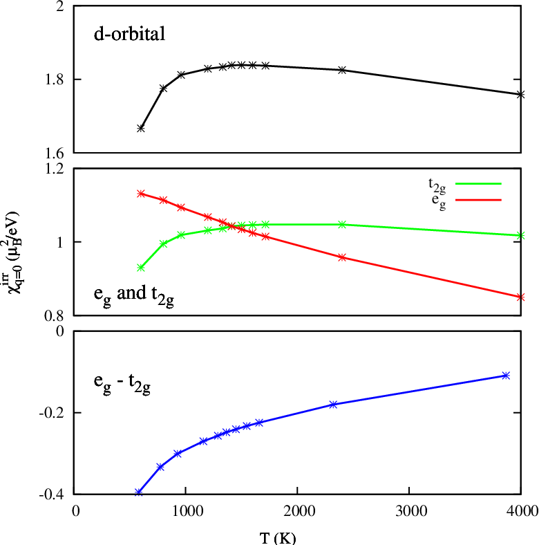
In order to analyze the role of peculiarities of band structure on non-monotonous temperature behavior of $\chi(T)$, we calculate $\chi^{\rm irr}_{\mathbf{q}=0}(T)$ projected onto pair sets of orbitals as in Eq. 6. The results are shown in Fig. 11 and inset of the Fig. 10. The overall temperature dependence of $\chi^{\rm irr}_{\mathbf{q}=0}(T)$ repeats that of $\chi(T)$, being however substantially weaker. The $t_{2g}$ contribution to $\chi^{\rm irr}_{\mathbf{q}=0}$ has a maximum at the temperature $T\sim 2000$ K, at which the energy of the thermal fluctuations becomes comparable to the distance of the peak of the $t_{2g}$–projected DOS to the Fermi level, which is about 0.3 eV. The origin of the maximum of $\chi^{{\rm irr},t_{2g}}_{\mathbf{q}=0}$ is also similar to that, analyzed recently for pnictides[44]. The $e_{g}$-$t_{2g}$ contribution has at $T<1000$ K the temperature dependence similar to that of $t_{2g}$ contribution but with a negative sign. The contribution of $e_{g}$ orbitals decreases almost linearly with increasing temperature. This is connected with strong (in comparison with $t_{2g}$ orbitals) correlated character of $e_{g}$ orbitals. Such a distinct behavior of different orbitals contributions results in the shift of maximum of total $d$-orbital irreducible susceptibility to approximately the temperature $T^{*}$, making it close to the position of uniform susceptibility maximum. The temperature $T^{*}$ is approximately equal to the characteristic temperature, discussed in Sect. II, above which the formaltion of local magnetic moments in $\gamma$-iron is expected, explaining naturally a crossover from Pauli-like to Curie-Weiss-like temperature dependence of the magnetic susceptibility. The ratio of total uniform susceptibility and irreducible one (Stoner enhancement factor) at $T\sim 1290$ K is about 10. It means that ferromagnetic fluctuations, which occur due to proximity of the Fermi level to the peak of the density of states, are strong in the temperature interval in the vicinity of $T^{*}$. Such a large ratio also explains strong temperature dependence of $\chi(T)$ in comparison with $\chi^{\rm irr}_{\mathbf{q}=0}(T)$.

To estimate exchange interactions we perform the mapping of the considered electronic system to the effective Heisenberg model. Due to presence of different competing magnetic orders we consider a rough way to extract the exchange integrals using the electronic properties in the paramagnetic phase at finite temperature. To this end we compare a momentum dependence of the static magnetic susceptibility, $\chi_{\mathbf{q}}$, obtained for the effective Heisenberg model with exchange parameters $J_{\mathbf{q}}$ within the $1/z$-expansion ($z$ is the coordination number) [49],

with the Eq. (7), which yields

Using the results for $\chi_{\mathbf{q}}^{\rm irr}$ within the LDA+DMFT method one can obtain the constant in the Eq. (12) if one fixes $J_{\mathbf{q}}$ by the condition $\sum_{\mathbf{q}}J_{\mathbf{q}}=0$. At $T=1290$ K we obtain $J_{\mathbf{q}=0}=\min_{\mathbf{q}}J_{\mathbf{q}}=-2380\,\text{K}$ and $J_{\mathbf{q}=\mathbf{q}_{\rm X}}=\max_{\mathbf{q}}J_{\mathbf{q}}=1172\,\text{K}$.

We have considered the electronic and magnetic properties of paramagnetic $\gamma$–iron. The shift of the DOS peak below the Fermi level in $\gamma$-iron causes the dramatic difference in the electronic and magnetic properties between $\alpha$- and $\gamma$-iron. The position of this peak is therefore crucial for understanding the magnetic properties which is similar to recent study of pnictides [44].

The account of correlation effects in $\gamma$–iron allows one to conclude that the effective local moments are formed in this material at sufficiently large temperature $T>\mbox{1000 K}$ with $\mu_{\rm loc}\approx 3.8\mu_{\rm B}$. The corresponding inverse local susceptibility $\chi_{\rm loc}^{-1}$ has however apart from the $T$-linear term also constant contribution, providing strong temperature dependence of the effective local moment $\mu_{\rm eff}=\sqrt{3T\chi_{\rm loc}}$, which in the temperature range 1200–1400 K is approximately $3\mu_{\rm B}$. At lower temperatures $\gamma$-iron is found to be better described in terms of itinerant picture.

The antiferromagnetism of $\gamma$–iron can be understood as occuring due to band structure features (nesting of some sheets of the Fermi surface, connecting $e_{g}$–$e_{g}$and $e_{g}$–$t_{2g}$ states). The obtained antiferromagnetic state with the wavevector close to $(2\pi/a)(1,0,0)$ is found to compete strongly with the other incommensurate spin-density wave instabilities. Observed tendency to the magnetic frustration can explain the small Néel temperature of $\gamma$–iron.

The application of obtained results for explaining $\alpha$-$\gamma$ structural transition in iron and the properties of some iron alloys with fcc structure is of further importance.

The authors are grateful to Yu. N. Gornostyrev, A. V. Korolev, A. N. Ignatenko and I. V. Leonov for useful discussions. This work was supported by the Russian Foundation for Basic Research (Projects Nos. 13-02-00050, 13-03-00641, 12-02-91371-CT a, 12-02-31207, 11-02-00931-a, 11-02-00937-a, 12-02-31510-mol-a, 10-02-91003-ANF a, the fund of the President of the Russian Federation for the support of scientific schools NSH-6172.2012.2, the Programs of the Russian Academy of Science: ”Quantum microphysics of condensed matter” (No. 12-P-2-1017, 12-CD-2), ”Strongly correlated electrons in solids and structures” (No. 12-T-2-2001); the grants of the Ministry of education and science of Russia No. 12.740.11.0026 and 14.A18.21.0076, the Program of ”Dynasty” foundation. Calculation were performed using “Uran” supercomputer of IMM UB RAS.

In this Appendix we consider the contribution of the low-frequency part of the local susceptibility (which is presumably responsible for contribution of localized degrees of freedom), described by the Eq. (2), to the instaneous local moment. Performing analytical continuation of the Eq. (2) to the imaginary frequency axis with the subsequent summation over Matsubara frequencies, we obtain:

where $n_{\rm m}\sim I/(2\pi T)$ is the largest frequency number, to which the behavior of Eq. (2) extends, and $\psi$ is the digamma function. It can be also estimated, that the high-energy part of the susceptibility yields only subleading contribution $O(\delta/(\pi T))$ to the Eq. (13). In Eq. (13) we can distinguish two regimes. First, if $\delta\ll\pi T,$ we find $\langle(S^{z})^{2}\rangle\simeq\mu_{\rm eff}^{2}/3,$ i.e. the instaneous local moment and the effective moment, extracted from the Curie law for local susceptibility are close to each other. This is identified with the (sufficiently long-living) local moment regime in main text. On the other hand, for $\delta\gtrsim\pi T$ we find $\langle(S^{z})^{2}\rangle\gg\mu_{\rm eff}^{2}/3,$ which corresponds to the itinerant regime.

References

- [1] Z. S. Basinski, W. Hume-Rothery, and A. L. Sutton, Proc. R. Soc. London, Ser. A 229, 459 (1955).
- [2] Constitution of Binary Alloys, edited by M. Hansen, McGraw-Hill, New York, 1958.
- [3] J. Donohue, The Structure of the Elements, J. Wiley & Sons Ltd., New York, 1974.
- [4] R. Kohlhaas, P. Dunner, N. Schmitz-Pranghle, Z. Angew. Phys. 23, 245 (1967).
- [5] S.V. Okatov, A.R. Kuznetsov, Yu.N. Gornostyrev, V.N. Urtsev, M.I. Katsnelson, Phys. Rev. B 79, 094111 (2009).
- [6] I. Leonov, A. I. Poteryaev, V. I. Anisimov, D. Vollhardt, Phys. Rev. Lett. 106, 106405 (2011).
- [7] I. Leonov, A. I. Poteryaev, V. I. Anisimov, D. Vollhardt, Phys. Rev. B 85, 020401 (2012).
- [8] F. Körmann, A. Dick, B. Grabowski, T. Hickel, and J. Neugebauer, Phys. Rev. B 85, 125104 (2012).
- [9] A. A. Katanin, A. I. Poteryaev, A. V. Efremov, A. O. Shorikov, S. L. Skornyakov, M. A. Korotin, V. I. Anisimov, Phys. Rev. B 81, 045117 (2010).
- [10] G. Borghi, M. Fabrizio, and E. Tosatti, ArXiv:1307.5738 (unpublished).
- [11] S. Arajs, D. S. Miller, J. Appl. Phys. 31, 986 (1960).
- [12] M. C. Gao, T. A. Bennett, A. D. Rollett and D. E. Laughlin, J. Phys. D: Appl. Phys. 39, 2890 (2006).
- [13] S. C. Abrahams, L. Guttman and J. S. Kasper. Phys. Rev. 127, 2052 (1962).
- [14] U. Gonser, C. J. Meechan, A. H. Muir, H. Wiedersich, J. Appl. Phys. 34, 2373 (1963).
- [15] G. J. Johanson, M. B. McGirr, D. A. Wheeler, Phys. Rev. B 1, 3208 (1970).
- [16] C. M. Liu and R. Ingalls, J. Appl. Phys. 50, 1751 (1979).
- [17] Y. Tsunoda, J. Phys.: Cond. Matt. 1, 10427 (1989).
- [18] T. Naono and Y. Tsunoda, J. Phys.: Cond. Matt. 16, 7723 (2004)..
- [19] Y. Tsunoda and N. Kunitomi, Y. Tsunoda and N. Kunitomi, J. Phys. F: Met. Phys. 18, 1405 (1988).
- [20] Y. Tsunoda, N. Kunitomi, and R. M. Nicklow, J. Phys. F: Met. Phys. 17, 2447 (1987).
- [21] K. P. Gupta, C. H. Cheng, and P. Beck: J. Chem Solids, 25, 73 (1964).
- [22] O.N. Mryasov, A.I. Liechtenstein, L.M. Sandratskii, and V.A. Gubanov, J. Phys.: Cond. Matt. 3, 7683 (1991).
- [23] M. Uhl, L.M. Sandratskii, and J. Kübler, J. Magn. Magn. Mater. 103, 314 (1992).
- [24] P. James, O. Eriksson, B. Johansson and I.A. Abrikosov, Phys. Rev. B 59, 419 (1999).
- [25] V.P. Antropov, M.I. Katsnelson, M. van Schilfgaarde, and B.N. Harmon, Phys. Rev. Lett. 75 729 (1995); V.P. Antropov, M.I. Katsnelson, B.N. Harmon, M. van Schilfgaarde, and D. Kuznezov, Phys. Rev. B 54, 1019 (1996).
- [26] M. Körling and J. Ergon, Phys. Rev. B 54, 8293 (1996).
- [27] K. Knöplfe, L.M. Sandratskii, and J. Kübler, Phys. Rev. B 62, 5564 (2000).
- [28] E. Sjöstedt and L. Nordström, Phys. Rev. B 66 014447 (2002).
- [29] I.A. Abrikosov, A.E. Kissavos, F. Liot, B. Alling, S.I. Simak, O. Peil, and A.V. Ruban, Phys. Rev. B 76, 014434 (2007).
- [30] S.V. Okatov, Yu.N. Gornostyrev, A.I. Lichtenstein, and M.I. Katsnelson, Phys. Rev. B 84, 214422 (2011).
- [31] A.V. Ruban, M.I. Katsnelson, W. Olovsson, S.I. Simak, and I.A. Abrikosov, Phys. Rev. B 71 054402 (2005).
- [32] S. Shallcross, A. Kissavos, S. Sharma, and V. Meded, Phys. Rev. B 73, 104443 (2006). on the density functional theory.
- [33] L. V. Pourovskii, T. Miyake, S. I. Simak, A. V. Ruban, L. Dubrovinsky, and I. A. Abrikosov, Phys. Rev. B 87, 115130 (2013).
- [34] R. O. Jones and O. Gunnarsson, Rev. Mod. Phys. 61, 689 (1989).
- [35] O. K. Andersen and O. Jepsen, Phys. Rev. Lett. 53, 2571 (1984).
- [36] U. von Barth and L. Hedin, J. Phys. C 5, 1629 (1972).
- [37] S. V. Vonsovskii, M. I. Katsnelson, and A. V. Trefilov, Fiz. Met. Metalloved. 76 (3) 3 (1993); 76 (4), 3 (1993).
- [38] R. Maglic, Phys. Rev. Lett. 31, 546 (1973).
- [39] V. I. Anisimov, D. E. Kondakov, A. V. Kozhevnikov, I. A. Nekrasov, Z. V. Pchelkina, J. W. Allen, S.-K. Mo, H.-D. Kim, P. Metcalf, S. Suga, A. Sekiyama, G. Keller, I. Leonov, X. Ren, and D. Vollhardt, Phys. Rev. B 71, 125119 (2005).
- [40] F. Lechermann, A. Georges, A. Poteryaev, S. Biermann, M. Posternak, A. Yamasaki, and O. K. Andersen, Phys. Rev. B 74, 125120 (2006).
- [41] A. I. Lichtenstein, M. I. Katsnelson, and G. Kotliar, Phys. Rev. Lett. 87, 067205 (2001).
- [42] J. E. Hirsch and R. M. Fye, Phys. Rev. Lett. 56, 2521 (1986).
- [43] A. Sandvik, Phys. Rev. B 57, 10287 (1998).
- [44] S. L. Skornyakov, A. A. Katanin, V. I. Anisimov, Phys. Rev. Lett. 106, 047007 (2011); S. L. Skornyakov, V. I. Anisimov, D. Vollhardt, Phys. Rev. B 86, 125124 (2012).
- [45] K. Hirai, J. Phys. Soc. Jpn. 58, 4288 (1989).
- [46] F. J. Pinski, J. Staunton, B. L. Gyorffy, D. D. Johnson, and G. M. Stocks, Phys. Rev. Lett. 56, 2096 (1986).
- [47] T. Moriya, Spin fluctuations in itinerant magnets. Springer-Verlag, Berlin, Heidelberg, 1985.
- [48] A. S. Belozerov, A. I. Poteryaev, and V. I. Anisimov, Phys. Rev. B 85, 045109 (2012).
- [49] Yu.A. Izyumov, F.A.Kassan-Ogly, and Yu.N.Skryabin, Field Methods in the Theory of Ferromagnetism [in Russian], Nauka, Moscow, 1974; Yu.A. Izyumov and Yu.N.Skryabin, Statistical Mechanics of Magnetically Ordered Substances, Consultants Bureau, New York, 1988