Virial expansion for a strongly correlated Fermi system and its application to ultracold atomic Fermi gases
Abstract
Strongly correlated Fermi system plays a fundamental role in very different areas of physics, from neutron stars, quark-gluon plasmas, to high temperature superconductors. Despite the broad applicability, it is notoriously difficult to be understood theoretically because of the absence of a small interaction parameter. Recent achievements of ultracold trapped Fermi atoms near a Feshbach resonance have ushered in enormous changes. The unprecedented control of interaction, geometry and purity in these novel systems has led to many exciting experimental results, which are to be urgently understood at both low and finite temperatures. Here we review the latest developments of virial expansion for a strongly correlated Fermi gas and their applications on ultracold trapped Fermi atoms. We show remarkable, quantitative agreements between virial predictions and various recent experimental measurements at about the Fermi degenerate temperature. For equation of state, we discuss a practical way of determining high-order virial coefficients and use it to calculate accurately the long-sought third-order virial coefficient, which is now verified firmly in experiments at ENS and MIT. We discuss also virial expansion of a new many-body paramter - Tan’s contact. We then turn to less widely discussed issues of dynamical properties. For dynamic structure factor, the virial prediction agrees well with the measurement at the Swinburne University of Technology. For single-particle spectral function, we show that the expansion up to the second order accounts for the main feature of momentum-resolved rf-spectroscopy for a resonantly interacting Fermi gas, as recently reported by JILA. In the near future, more practical applications with virial expansion are possible, owing to the ever-growing power in computation.
pacs
05.30.Jp, 03.75.Mn, 67.85.Fg, 67.85.Jk; Keywords: Ultracold atomic Fermi gas, virial expansion, Feshbach resonance, thermodynamics, virial coefficientI Introduction
I.1 Universal strongly correlated Fermi systems: From dilute neutron matter to ultracold trapped Fermi atoms
The strongly correlated Fermi gas is a ubiquitous system in nature [1]. It appears in the quark-gluon plasmas in the early Universe [2], neutron stars [3, 4], high-temperature superconductors [5], and most recently in ultracold atoms [6, 7, 8] (see Fig. 1). The strong correlation is a result of a large separation of length scales and the Fermi system is close to an interesting universal limit with infinitely large scattering length and zero effective range of interaction [9, 10]. The absence of length scale implies that the type and detail of interactions are not important. It is anticipated that universal behaviors in both static and dynamic properties would emerge [10, 11, 12].

Dilute neutron matter is a good example of strongly-correlated Fermi systems [3, 4]. The neutron scattering length is about fm and the effective range is fm . For typical neutron densities , where fm-3 is the saturation density of nuclear matter, the dimensionless interaction parameter while is small. Here, is the Fermi wave-vector. Therefore, the neutron matter is close to the unitary limit, with which the s-wave scattering amplitude becomes saturated at a zero-energy resonance. Understanding the nuclear matter appears to be a challenging many-body theoretical problem [13, 14].
In this context, a unitary atomic Fermi gas realized recently in ultracold atom laboratory attracts particular attention [6, 7, 8]. It serves as a new paradigm for studying strong-correlations because of its unprecedented controllability and purity. By tuning an external magnetic field across a collisional Feshbach resonance [15], the interatomic attractions in a two-component Fermi gas can be changed precisely from weak to infinitely strong, leading to the observation of crossover from Bardeen-Cooper-Schrieffer (BCS) superfluids to Bose-Einstein condensates (BEC) [16, 17], which was anticipated long time ago [18, 19, 20]. At the resonance, the s-wave scattering length is exactly infinity and the effective range of interaction is negligible. This unitary limit can now be routinely achieved in laboratories with fermionic potassium-40 (40K) [16] and lithium-6 (6Li) atoms [17].
Experimentally, the near resonance regime was first approached by O’Hara et al. in 2002 with 6Li atoms [21]. The stability of atomic Fermi gases under strong attractions was observed and the ground state energy was found to reduce significantly with respect to that of an ideal, non-interacting Fermi gas. Since then, a number of different aspects of a unitary Fermi gas have been characterized after substantial experimental efforts. Hydrodynamic ballistic expansion and collective excitations due to strong correlations were confirmed [22, 23, 24]; superfluidity at BEC-BCS crossover was unambiguously verified by generating quantized vortices [25]; universal thermodynamics was evidenced by heat capacity measurement [11, 26, 27, 28, 29, 30, 31, 32]; nearly ideal hydrodynamic flow and universal viscosity was observed [33]. Recently, these studies have been extended to Fermi gases with unequal densities for the spin-up and spin-down components [34, 35] and to Fermi gases in low-dimensions [36, 37, 38], giving the prospects of realizing exotic inhomogeneous Fulde-Ferrell-Larkin-Ovchinnikov (FFLO) superfluidity [39, 40, 41, 42] and Berezinskii-Kosterlitz-Thouless (BKT) transition [43, 44, 45]. Along with rapid experimental progress, new measurement techniques have been developed to characterize strongly correlated Fermi gases. These include the momentum-resolved rf-spectroscopy for measuring single-particle spectral function [46, 47] and the two-photon Bragg spectroscopy for dynamic and static structure factors [48].
In contrast, the parallel theoretical development is much slower. There are numerous activities on developing better strong-coupling theories [20, 49, 50, 51, 52, 53, 54, 55, 56, 57, 58] or ab-initio quantum Monte Carlo (QMC) methods [59, 60, 61, 62, 63, 64]. However, a deep understanding of strongly correlated Fermi gases is prohibited because of the absence of a controllable small interaction parameter. The use of standard strong-coupling theories requires infinite order expansions and the truncation to a particular order can not be fully justified a priori [65, 66]. At this stage, numerically exact QMC simulations are less accurate than one might expect, suffering from either the notorious sign problem for fermions [61] or the finite size effects in small samples used in the simulation [60, 62].
In this respect, exact results of strongly correlated Fermi gases in some non-trivial limits are very valuable. Two recent efforts are notable. In the limit of short-distance, large-momentum, and/or large-frequency, Tan derived a set of exact universal relations [67, 68]. It was shown that all the limiting behaviors are governed by a many-body parameter called the contact, which measures the density of pairs within short distances. Tan’s relations can be conveniently understood using the short-distance and/or short-time operator product expansion (OPE) method [69], which separates in a natural way the few-body physics from many-body physics. In another limit of high temperature, quantum virial expansion [70, 71, 72, 73, 74, 75, 76, 77, 78, 79] provides another rigorous means to bridge few-body and many-body physics. The properties of a strongly correlated Fermi gas, either static [70, 72, 73, 77, 78] or dynamic [75, 76], can be expanded non-perturbatively using some exact expansion coefficients or expansion functions, which are calculable from few-fermion solutions [80, 81, 82, 83, 84, 85, 86]. Both Tan relations and virial expansion give useful insights into the challenging many-body problem, though in the different perspective.
In this paper, we review the recent theoretical development on quantum virial expansion, and show that virial expansion gives a complete solution of strongly-correlated Fermi gas above the Fermi degenerate temperature. We focus our attention on ultracold atomic Fermi gases, and compare in a quantitative way the virial expansion predictions with available experimental measurements for various fundamental properties. We note that the virial expansion has also been used frequently to study the equation of state of neutron matter [87, 88, 89, 90, 91, 92].
I.2 Overview of virial expansion picture
Quantum virial expansion, alternatively referred to as quantum cluster expansion, is a standard method in quantum statistical mechanics [93, 94]. It is practically useful for a dilute quantum gas. The basic idea of virial expansion is simple. Though we have a strongly correlated system at low temperatures, with increasing temperature the correlation between particles would become increasingly weak. At sufficiently high temperatures, the scattering cross section is of the order the square of the thermal de Broglie wavelength, which becomes much smaller than the average inter-atomic distance. As a result, the inclusion of few-body correlations is already sufficient to describe the underlying properties of the system. These few-body correlations can be exactly taken into account using few-particle solutions and virial expansion.
As a concrete example, let us consider the thermodynamic potential for a given Hamiltonian , which in the grand canonical ensemble is given by [95],
| (1) |
where is the Boltzmann constant,
| (2) |
is the grand partition function, and is the field operator of total number of particles. The thermodynamic potential can be written in terms of the partition function of clusters,
| (3) |
where the integer denotes the number of particles in the cluster and the trace Trn is taken over -particle states with a proper symmetry. is calculable using the complete solutions of a -particle system. The grand partition function then takes the form
| (4) |
where is the fugacity [95]. At large temperatures, it is well-known that the chemical potential diverges to , so the fugacity would be very small, . By Taylor-expanding in powers of the small fugacity, it is obvious that
| (5) |
where can be expressed in terms of () and therefore contains the contribution from few-body physics up to -particles.
In principle, all the properties of a quantum gas could be cluster expanded in powers of fugacity, no matter how strong the interactions. The fugacity is a natural small parameter at large temperatures. Naïvely, virial expansion is applicable when . For a two-component spin-1/2 Fermi gas, using the fact that the fugacity is roughly equal to the phase-space density , where is the density, is the thermal de Broglie wavelength and the mass of atoms, one can estimate that virial expansion is useful at temperature . Here is the Fermi degenerate temperature.

Though virial expansion is a large-temperature expansion, it has an intrinsic relation with low-temperature strong-coupling diagrammatic theory. In the absence of a small interaction parameter, we may conjecture that a reliable strong-coupling theory of strongly correlated systems should be developed by successively including few-particle scattering process. Thus, we may write
| (6) |
where is the thermodynamic potential of a non-interacting system, and () is the contribution from the -particle scattering process, which is to be calculated at all temperatures by summing a series of diagrams to infinite order (i.e., the -particle vertex function ). We shall refer to such an expansion as the diagrammatic expansion. As an example, in Fig. 2 we show the diagrammatic representation of . It sums up all the two-particle scatterings via the two-particle vertex function [18]. In the language of functional path-integral method, corresponds to the gaussian fluctuations around the mean-field saddle point [18, 19, 20, 53]. It is obvious that at large temperatures, by expanding () in powers of , we can calculate directly appeared in the virial expansion. In this respect, virial expansion and diagrammatic expansion are closely related. Both of them are the expansion in few-particle correlations. The advantage of the diagrammatic expansion is that it takes into account the few-particle scatterings in the medium, and therefore is applicable at all temperatures. It is a natural generalization of virial expansion to the low-temperature regime. These two expansion theories are sketched in Fig. 3.

Ideally, for a strongly correlated system, we anticipate that becomes less important with increasing and the diagrammatic expansion thus converges. Indeed, for a unitary Fermi gas at the BEC-BCS crossover, the theoretical calculation of at zero temperature gives fairly accurate equation of state [53], as confirmed by the latest experimental measurement [96]. Others terms of with are notoriously difficult to obtain, but are conjectured to be small at low temperatures. Virial expansion provides systematic determinations of at high temperatures and may shed light on their low temperature behavior.
At this point, we may anticipate that the applicability of virial expansion is not limited to small fugacity . The expansion could be meaningful in the deep quantum degenerate regime through an analytic continuation across the point , and therefore is applicable down to the superfluid phase transition temperature . The pursuit of such an improved virial expansion theory is a theoretical challenge.
I.3 Key technical issues in the latest development of virial expansion
Despite the usefulness of virial expansion, its application to strongly correlated quantum gases is less documented in the literature. There are two severe technical difficulties in applying virial expansion to a homogeneous system: (i) insufficient knowledge on the exact few-particle solutions and (ii) continuous energy spectrum. As a result, it seems impossible to calculate the essential few-particle cluster partition function when , as the calculation requires infinitely large number of energy levels. Therefore, previous applications of virial expansion have been restricted to the second order, where can be calculated using an elegant phase-shift formalism derived by Beth and Uhlenbeck in 1937 [97, 98].
The latest development of virial expansion, to be reviewed in this paper, relies on the recent theoretical progress on the exact few-particle solutions of trapped strongly interacting fermions [80, 81, 82, 83, 84, 85, 86]. Due to the trapping potential, the energy spectrum becomes discrete. As the thermal energy provides a natural high-energy scale in the cluster partition function, the number of energy levels required by the calculation is finite. In principle, we can always calculate numerically these energy levels using the ever-growing computation power, if few-particle solutions are not known analytically. In addition, virial expansion of dynamic properties becomes possible, based on the calculated few-particle wave-functions [75, 76].
To get back to the homogeneous system, one can utilize the so-called local density approximation, which treats the trapped Fermi gas as a collection of many locally uniform blocks. In the unitary limit, it is found that the virial expansion results for trapped and homogeneous systems are convertible by some universal relations [72, 12]. The details will be discussed later.
I.4 Model Hamiltonian
Throughout this Review, we focus on the strongly-interacting Fermi gases with zero-range interactions in three dimensions, which have emerged as the simplest strongly-correlated model system that has been accessed experimentally with ultracold atoms of 6Li and 40K [6, 7, 8]. They also serve as a “bare bone” description of nuclear and neutron matter. The generalization of virial expansion in low dimensional systems is straightforward [74].
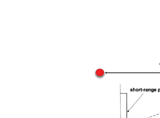
The use of zero-range interactions can be understood from Fig. 4, which plots the short-range behavior of the zero-energy scattering wave-function for real interatomic interactions with a range of interactions . For an ultracold dilute Fermi gas, is typically at the order of m, much smaller than the mean inter-particle distance m. As a result, the complicated short-range behavior of the wave-function, which corresponds to high-energy physics, becomes irrelevant for typical atomic collisions. Therefore, we may set effectively and approximate at [94]. Here is the -wave scattering length [94]. This is the so-called Bethe-Peierls (BP) boundary condition, which is equivalent to the -wave zero-range interactions (or the so-called pseudopotential [94]). We note that, when the -wave scattering length becomes positive, the interaction potential will support a two-body bound state with energy . Therefore, in the unitary limit, where , a shallow two-body bound state with infinitely small energy emerges. For more details, see ref. [15].
In the ultracold atom experiments, a harmonic trap is necessary to prevent atoms from escaping. We thus consider fermions in a three-dimensional isotropic harmonic trap with the same mass and trapping frequency , occupying two different hyperfine states or two spin states. The zero-range -wave interaction between fermions with unlike spins is replaced by the BP boundary condition. That is, when any particles and with unlike spins are close to each other, , the many–body wave function with proper symmetry should satisfy [99, 100],
| (7) |
where is a function independent of . This BP boundary condition can be equivalently written as,
| (8) |
Otherwise, the wave function obeys a non-interacting Schrödinger equation,
| (9) |
In the second quantization, the system can be instead described by the model Hamiltonian,
| (10) |
where the chemical potentials and could be different due to unequal spin-populations. The zero-range interaction is given by a contact potential . The bare interaction strength is to be renormalized by two-particle vertex function in the vacuum [95], using
| (11) |
where the momentum has a high-energy cut-off, , in accord with the use of zero-range interactions. scales to zero as the cut-off momentum .
I.5 Brief introduction to Tan relations
Here we introduce briefly the exact Tan relations, which were derived by Shina Tan in 2005 [67, 68]. These Tan relations link the asymptotic behavior of many-body systems at short-range, large-momentum, and high-frequency to their thermodynamic properties. For instance, the momentum distribution falls off as at large momentum, the pair correlation function diverges like
| (12) |
and the rf-spectroscopy has the tail of at large frequency [103, 104]. All the Tan relations are related to each other by a single coefficient , referred to as the integrated contact density or contact. The contact measures the probability of two fermions with unlike spins being close together [69]. It also links the short-range behavior to thermodynamics via the adiabatic relation,
| (13) |
which gives the change in the total energy due to adiabatic changes in the scattering length. The fundamental importance of the Tan relations arises from their wide applicability. They are useful at both zero or finite temperature, superfluid or normal phase, homogeneous or trapped, few-body or many-body systems.
While the original rigorous derivation by Shina Tan is difficult to follow, the underlying physics of Tan relations can be easily understood from several points of view [68]. The simplest way is from the two-body wave function under the BP boundary condition, . Naïvely, the momentum distribution is simply the square of the Fourier transform of and the pair correlation function . The asymptotic behavior of and is then straightforward to check.
At the many-body level, Tan’s relations can be elegantly proved by using the short-distance and/or short-time operator product expansion (OPE) method [69], in which the contact is identified as
| (14) |
For example, the adiabatic relation Eq. (13) can be obtained directly by applying Hellmann-Feynman theorem to the model Hamiltonian [69],
| (15) |
The last step follows the renormalization for the bare interaction strength Eq. (11).
The contact is a fundamental parameter that characterizes the many-body properties of strongly correlated Fermi gases. Recently, its measurement receives considerable attentions [105, 106, 107, 108]. It turns out that the most accurate way is through the Tan relation for spin-antiparallel static structure factor [109], which is obtained by a direct Fourier transform of pair correlation function,
| (16) |
The simple power-law tail of in the structure factor relation is more amenable for experimental measurement than the or tail in the momentum distribution or in rf-spectroscopy. In the latter two cases, the fast decay due to the higher-order power law imposes more stringent signal-to-noise requirements at a given momentum or frequency. Experimentally, the static structure factor can be measured by two-photon Bragg spectroscopy [48, 106].
I.6 Brief summary of virial expansion results
We now summarize briefly the main results of the latest development in virial expansion. In general, thermodynamic properties such as the thermodynamic potential can be expanded in terms of some virial coefficients, while dynamic properties, i.e., the single-particle spectral function and dynamic structure factor, can be expanded in terms of some virial expansion functions. The latest developments of virial expansion include:
(i) The third virial coefficient for thermodynamic potential has been precisely determined [72, 78]. For a homogeneous Fermi gas in the unitary limit, it is found that [78]. Here is the third virial coefficient of an ideal, non-interacting Fermi gas. This theoretical prediction has been confirmed experimentally with the experimental value [30] and has been independently checked by a field theoretic approach [110], which gives . The fourth virial coefficient in the unitary limit has also been calculated [78], but with much less accuracy, . The virial coefficients of a trapped system and a homogeneous system are related by [72], (). These virial coefficients predict an accurate equation of state for a trapped Fermi gas in the unitary limit, for temperature down to [66]. We review the virial expansion of thermodynamics in Sec. II.
(ii) The contact parameter can be virial expanded in terms of contact coefficients [77]. For a homogeneous Fermi gas in the unitary limit, it is predicted that and [110]. In analogy with the virial coefficient, the contact coefficients of a trapped system and a homogeneous system are related by, . Likewise, for a trapped Fermi gas in the unitary limit, the virial expansion of contact provides an excellent explanation for the experimental measurement at [107]. This part will be reviewed in Sec. III.
(iii) The virial expansion functions for the single-particle spectral function and dynamic structure factor have been determined [75, 76], to the second order in fugacity. These results enable an important qualitative understanding of recent experimental measurements on momentum-resolved rf-spectroscopy [46, 47] and two-photon Bragg spectroscopy [107, 108], for a trapped Fermi gas in the unitary limit at temperature down to the superfluid transition. The determination of the third virial expansion functions is straightforward, but involves much heavier numerical efforts. The virial expansion of dynamic structure factor and of single-particle spectral function will be reviewed in Secs. IV and V, respectively.
II Virial expansion of equation of state
Let us consider the virial expansion of the thermodynamic potential , for a balanced spin-1/2 Fermi gas with equal spin populations (). The spin-population imbalanced case with will be discussed at the end of the section. All the equations of state can be derived from the thermodynamic potential. By Taylor-expanding in the fugacity, where , the thermodynamic potential takes the form,
| (17) |
where is referred to as the -th (virial) expansion coefficient. Note that, by definition in Eq. (5) is given by . It is readily seen that,
| (18) | |||||
| (19) |
These equations give a general definition of virial expansion, which is applicable to both homogeneous and trapped systems. The calculation of the -th virial coefficient requires the input of cluster partition function (), and hence requires the solutions of up to the -particle problem. In practice, it is convenient to concentrate on the interaction effects only. We therefore consider the difference and , where the superscript “’’ denotes the non-interacting systems 11 1 We note that there are varying definitions of virial coefficients in the literature. In some works, e.g. ref. [30], the ideal gas contribution is excluded from the definition of virial coefficients. That is, defined in the present work is treated as the virial coefficient .. For the second and third virial coefficients, one shall calculate respectively
| (20) |
and
| (21) |
As we mentioned earlier, the calculation of virial coefficients in the strongly correlated regime is a subtle theoretical problem. The second virial coefficient was known long time ago through the elegant Beth-Uhlenbeck formalism, which relates in a simple manner the second virial coefficient to the two-body -matrix or the two-body scattering phase shift [97, 98, 111]. A connection between the virial series and the scattering matrix has been suspected since then. However, the computation of the third virial coefficient, along the line of Beth and Uhlenbeck’s original work, met the very difficulties of the three-particle problem [112, 113].
Until very recently, there is renewed interest in calculating higher-order virial coefficients, largely due to the creation of ultracold atomic Fermi gases. Initial attempt was based on the field theoretic method, by calculating the contribution of three-particle scattering process to the thermodynamic potential [114]. It was shown by Rupak in 2007 that in the unitary limit, [115]. However, it was soon realized by Liu, Hu and Drummond [72] that this value does not agree with the high-temperature heat-capacity measurements reported by Thomas’s group at Duke University [29]. Using an entire different strategy based on Eq. (21) and the exact three-particle solution in harmonic traps, they predicted . The numerical accuracy of can be improved by including more three-particle energy levels. The latest calculation by Rakshit, Daily and Blume, along the line of Liu, Hu and Drummond’s work, gave and [78]. In parallel, new field theoretic calculations for the third virial coefficient have been performed. It was shown by Kaplan and Sun [116] and by Leyronas [110]. At this stage, more complete field theoretic calculation is desirable, in order to confirm independently the fourth virial coefficient and to predict new virial coefficients.
On the other hand, the experimental accuracy in measuring the equation of state of a unitary Fermi gas is improved very rapidly. The measurement by Salomon’s group at École Normale Supérieure (ENS) gave and [30]. The latest measurement by Zwierlein’s group at MIT reported [32]. We anticipate that the new predictions on the virial coefficients, improved continuously by many theorists, will play an important role in deepening our understanding of the equation of state of strongly correlated Fermi systems.
II.1 Virial coefficients of non-interacting Fermi gases
The background non-interacting virial coefficients can be conveniently determined by the non-interacting thermodynamic potential. For a homogeneous two-component Fermi gas, it takes the form [95],
| (22) |
where is the single-particle energy, the factor of accounts for the spin degree of freedom. By using and introducing a new variable , the ideal thermodynamic potential becomes,
| (23) |
where is the thermal de Broglie wavelength. It is easy to identify . Therefore, by Taylor-expanding in fugacity and integrating out term by term, we obtain the non-interacting virial coefficients in free space,
| (24) |
For a Fermi gas in a harmonic trapping potential , it is convenient to use the semiclassical approximation, or the so-called local density approximation. In the non-interacting limit, this amounts to setting,
| (25) |
where locally the single-particle energy is given by . Hereafter, we take the subscript “” to denote the quantity in the trapped system, otherwise, by default we refer to a homogeneous system. As before, the integrations over and can be done by introducing a new variable . This leads to,
| (26) |
where . By Taylor-expanding the log-term in fugacity , we find the non-interacting virial coefficients in harmonic traps,
| (27) |
We note that the use of semi-classical approximation means to neglect the discreteness of the energy spectrum in traps. Mathematically, this is equivalent to take a small parameter and to keep in the results the leading term in . We note also that the non-interacting virial coefficients in the homogeneous case and trapped case are related by, ().
II.2 Universal relation between homogeneous and trapped virial coefficients
The correspondence relation discussed in Sec. IIA holds for a strongly interacting Fermi gas as well. Here, the crucial point is that the virial coefficients become temperature independent. To understand this, we note that in general the coefficients should be a function of the ratio , between the only two length scales and . The temperature dependence enters through the thermal de Broglie wavelength. However, for a unitary Fermi gas where , this dependence disappears. This is indeed a manifestation of fermionic universality, shared by many quantum systems with strong short-range interactions.
In the thermodynamic limit, let us consider the thermodynamic potential of a harmonically trapped Fermi gas in the local density approximation,
| (28) |
where the trapped virial coefficients are to be determined and is the local thermodynamic potential,
| (29) |
Here, the local fugacity is given by the local chemical potential . Because of the temperature-independent (constant) virial coefficients , the spatial integration can be done explicitly. This immediately leads to the universal relation for the virial coefficients of a unitary Fermi gas,
| (30) |
II.3 Second virial coefficient of interacting Fermi gases
II.3.1 Beth-Uhlenbeck formalism
As shown by Beth and Uhlenbeck in 1937 [97], the second virial coefficient can be expressed in terms of the phase shifts of a two-body scattering problem. For a spin-1/2 Fermi gas, it takes the form,
| (31) |
where the first summation is over all the two-body bound states (with the energy ) and is the phase shift of the -th partial wave. The second virial coefficient therefore can be determined for arbitrary interatomic interactions. For a pedagogical explanation of the elegant Beth-Ulenbeck formalism, we refer to the classical book by Kerson Huang [94]. This formalism has been applied by Ho and Mueller to explore the universal properties of atomic gases near a Feshbach resonance at high temperatures [70]. It has also been used extensively to study the equation of state of nuclear and neutron matter [87, 88, 89, 90, 91, 92].
For a -wave Feshbach resonance that is of interest in ultracold atoms, the general expression for the -wave phase shift is [94, 98],
| (32) |
which leads to,
| (33) |
Here for general discussion we have kept a nonzero range of interactions, . It is easy to see that the main contribution to the integral in Eq. (31), , comes from the region . Thus, after introducing a new variable , the integral becomes,
| (34) |
In the case of zero-range approximation (), we obtain [70],
| (35) |
where and is the error function. The correction due to a finite range of interactions can be taken into account by Taylor-expanding the function in Eq. (34) in a series of . To the leading order, we find that,
| (36) |
Near a Feshbach resonance where and , we have,
| (37) |
In terms of the small dimensionless interaction strength () and the range of interactions (), the second virial coefficient can be written as,
| (38) |
where the single bound state exists only for a positive scattering length with its energy depending on both and . In the unitary limit, where , , and , we obtain the well-known result [94, 98],
| (39) |
Concerning the experimental measurement, as an example, we estimate the second virial coefficient for 6Li atoms using realistic experimental parameters. Let us consider the negative scattering length (BCS) side of the Feshbach resonance, for which the second virial coefficient takes the form,
| (40) |
The second and third terms on the right-hand-side of the above equation are non-universal since both of them depend on the temperature. These non-universal corrections are caused by a finite scattering length or a finite range of interactions.
For 6Li atoms, the finite scattering length near the Feshbach resonance G can be conveniently calculated using [118],
| (41) |
where in units of the Bohr radius m, and G. At the typical experimental density, where nm, we find that , if the magnetic field is tuned away from the resonance by one Gauss. This leads to about a percent correction to the second virial coefficient at the degenerate temperature . On the other hand, the finite range of interactions near the resonance can be modeled as [119],
| (42) |
where nm and nm is essentially the Van der Waals length. As across the Feshbach resonance, the finite range of interactions is reduced to a constant nm. Thus, we obtain the dimensionless range of interactions , for the typical Fermi wavelength. It gives about 0.1% correction to the second virial coefficient at .
II.3.2 Field theoretic method
The second virial coefficient can also be conveniently calculated using the field theoretic method [117], i.e., the diagrammatic expansion method we mentioned earlier in Sec.IB. This provide a simple example to illustrate the close relation between the virial expansion and the diagrammatic expansion. In the following, we introduce briefly the procedure. To obtain the virial coefficients, the basic idea of field theoretic method is to calculate , which is the contribution of -particle scattering process to the thermodynamic potential [115]. At large temperatures, we expand in fugacity,
| (43) |
where is the -th virial coefficient from -particle interaction. The total -th virial coefficient , where is the virial coefficient of an ideal Fermi gas. In the case of , we have .
We start from a path-integral functional action [19, 53], using the single-channel fermionic model with zero-range interactions Eq. (10). By performing a Hubbard-Stratonovich transformation to decouple the interaction term, the original fermionic partition function can be expressed as , in terms of bosonic variables . The “effective” bosonic action can be written in a series expansion: . In the normal state, the first term in the expansion reads [18, 19, 53],
| (44) |
where
| (45) |
is the two-particle propagator. Here we have used the abbreviation , the bosonic (fermionic) Matsubara frequency (), , and the Fermi distribution function . The action accounts for the scatterings between two-particles in the presence of other particles (i.e., medium), and thus includes the two-body contribution to all the virial coefficients of (). It gives rise to the following thermodynamic potential given by Nozières and Schmitt-Rink (NSR) in 1985 [18],
| (46) |
where the summation over the Matsubara frequency has been converted into an integral using a phase shift,
| (47) |
and is the Bose-Einstein distribution function. The diagrammatic representation of has been illustrated earlier in Fig. 1.
In the high-temperature limit, where the fugacity and , we may Taylor-expand the phase shift in powers of . Focusing on the unitary limit, we approximate the two-particle propagator
| (48) |
where
| (49) | |||||
| (50) |
and . To the leading order of , the phase shift is exactly a step function,
| (51) |
Thus, to the leading order of fugacity we have,
| (52) |
This gives rise to the second virial coefficient . Away from the unitary limit, it is straightforward to show that we can recover the Beth-Uhlenbeck formalism from Eq. (46), by taking the phase shift in vacuum.
We note that the higher-order contribution of () can be obtained by successively calculating the term in Eq. (46).
II.4 Virial coefficients from exact few-body solutions in harmonic traps
We now turn to calculate the third virial coefficient, by using an entirely different method [73]. We solve first the two-particle and three-particle problems in an isotropic 3D harmonic trap , and then use the solutions to obtain the second and third virial coefficients. In the end, we discuss the possibility of calculating the fourth virial coefficient.
We note that in cold-atom experiments the harmonic trap is often highly anisotropic. The three-particle problem at unitaritiy in an anisotropic trap can hardly be solved exactly. Fortunately, for a large number of particles, for which the local density approximation is valid, we are free to use harmonic traps of any aspect ratio to calculate the virial coefficients, by using the universal relation Eq. (30).
II.4.1 Relative Hamiltonian of few-particle systems
In a harmonic trap, it is useful to separate the center-of-mass motion and relative motion. We thus define the following center-of-mass coordinate and relative coordinates () for fermions in a harmonic trap [99, 100],
| (53) |
and
| (54) |
respectively. In this Jacobi coordinate, the Hamiltonian of the non-interacting Schrödinger equation takes the form , where,
| (55) |
and
| (56) |
The center-of-mass motion is simply that of a harmonically trapped particle of mass , with well-known wave functions and spectrum , where is a non-negative integer. In the presence of interactions, the relative Hamiltonian should be solved in conjunction with the Bethe-Peierls boundary condition, Eq. (8).
II.4.2 Two fermions in a 3D harmonic trap
Let us consider the two-fermion problem in a harmonic trap, where the relative Schrödinger equation becomes
| (57) |
where two fermions with unlike spins do not stay at the same position (). Here, we have re-defined and without confusing with the chemical potential we have used a reduced mass . It is clear that only the subspace of the relative wave function is affected by the -wave contact interaction. According to the Bethe-Peierls boundary condition, as the relative wave function should take the form, , or satisfy, . The two-fermion problem in a harmonic trap was first solved by Busch and coworkers [80]. In the following, we present a simple physical interpretation of the solution.
The key point is that, regardless of the boundary condition, there are two types of general solutions of the relative Schrödinger equation (57) in the subspace, . Here the function can either be the first kind of Kummer confluent hypergeometric function or the second kind of Kummer confluent hypergeometric function . We have taken as the characteristic length scale of the trap. In the absence of interactions, the first Kummer function gives rise to the standard wave function of 3D harmonic oscillators. With interactions, however, we have to choose the second Kummer function , since it diverges as at origin and thus satisfies the Bethe-Peierls boundary condition.
Therefore, the (un-normalized) relative wave function and relative energy should be rewritten as,
| (58) |
and
| (59) |
respectively. Here, is the Gamma function, the real number plays the role of a quantum number and should be determined by the boundary condition, . By examining the short range behavior of the second Kummer function , this leads to the familiar equation for energy levels [80],
| (60) |
In Fig. 5, we give the resulting energy spectrum as a function of the dimensionless interaction strength .

The spectrum is easy to understand. At infinitely small scattering length , (), which recovers the spectrum in the non-interacting limit. With increasingly attractive interactions, the energies decrease. In the unitarity (resonance) limit where the scattering length diverges, , we find that . As the attraction increases further, the scattering length becomes positive and decreases in magnitude. We then observe two distinct types of behavior: the ground state is a molecule of size , whose energy diverges asymptotically as as , while the excited states may be viewed as two repulsively interacting fermions with the same scattering length . Their energies decrease to the non-interacting values as .
In this two-body picture, a universal repulsively interacting Fermi gas with zero-range interaction potentials may be realized on the positive scattering length side of a Feshbach resonance for an attractive interaction potential, provided that all two fermions with unlike spins occupy the exited states or the upper branch of the two-body energy spectrum.

II.4.3 Three fermions in a 3D harmonic trap: General exact solutions
Let us turn to the three fermion case by considering two spin-up fermions and one spin-down fermion, i.e., the configuration shown in Fig. 6. The relative Hamiltonian can be written as [99, 100],
| (61) |
where we have redefined the Jacobi coordinates and , which measure the distance between the particle 1 and 2 (i.e., pair), and the distance from the particle 3 to the center-of-mass of the pair, respectively.
Inspired by the two-fermion solution, it is readily seen that the relative wave function of the Hamiltonian (61) may be expanded into products of two Kummer confluent hypergeometric functions. Intuitively, we may write down the following ansatz [72],
| (62) |
where,
| (63) |
The two-body relative wave function with energy describes the motion of the paired particles 1 and 2, and the wave function with energy gives the motion of particle 3 relative to the pair. Here, is the standard radial wave function of a 3D harmonic oscillator and is the spherical harmonic. Owing to the rotational symmetry of the relative Hamiltonian (61), it is easy to see that the relative angular momenta and are good quantum numbers. The value of is uniquely determined from energy conservation,
| (64) |
for a given relative energy . It varies with the index at a given angular momentum . Finally, is an exchange operator for particles 1 and 3, which ensures the correct exchange symmetry of the relative wave function due to Fermi exclusion principle, i.e., . The relative energy together with the expansion coefficient should be determined by the Bethe-Peierls boundary condition, i.e., . We note that the second Bethe-Peierls boundary condition in case of particle 2 approaching particle 3 is satisfied automatically due to the exchange operator acting on the relative wave function.
By writing , the Bethe-Peierls boundary condition takes the form (),
| (65) |
Using the asymptotic behavior of the second kind of Kummer function, , it is easy to show that in the limit of ,
| (66) |
and
| (67) |
Thus, the Bethe-Peierls boundary condition becomes,
| (68) |
where
| (69) |
Projecting onto the orthogonal and complete set of basis functions , we find that a secular equation,
| (70) |
where we have defined the matrix coefficient,
| (71) |
which arises from the exchange effect due to the operator . In the absence of , the above secular equation describes a three-fermion problem of a pair and a single particle, un-correlated to each other. It then simply reduces to Eq. (60), as expected.
The secular equation (70) was first obtained by Kestner and Duan by solving the three-particle scattering problem using Green function [82]. To solve it, for a given scattering length we may try different values of relative energy , implicit via . However, it turns out to be more convenient to diagonalize the matrix for a given relative energy, where
| (72) |
The eigenvalues of the matrix then gives all the possible values of for a particular relative energy. We finally invert to obtain the relative energy as a function of the scattering length. Numerically, we find that the matrix is symmetric and thus the standard diagonalization algorithm can be used. We outline the details of the numerical calculation of Eq. (72) in the Appendix A.
II.4.4 Three fermions in a 3D harmonic trap: Exact solutions in the unitarity limit
In the unitarity limit with infinitely large scattering length, , we may obtain more physical solutions using hyperspherical coordinates, as shown by Werner and Castin [81, 100]. By defining a hyperradius and hyperangles , where and and are respectively the unit vector along and , we may write [81, 100],
| (73) |
to decouple the motion in the hyperradius and hyperangles for given relative angular momenta and . It leads to the following decoupled Schrödinger equations [100],
| (74) |
and
| (75) |
where is the eigenvalue for the -th wave function of the hyperangle equation.
For three-fermions, is always positive. Therefore, the hyperradius equation (74) can be interpreted as a Schrödinger equation for a fictitious particle of mass unity moving in two dimensions in an effective potential with a bounded wave function . The resulting spectrum is [81, 100]
| (76) |
where the good quantum number labels the number of nodes in the hyperradius wave function.
The eigenvalue should be determined by the Bethe-Peierls boundary condition, which in hyperspherical coordinates takes the from [81, 100],
| (77) |
In addition, we need to impose the boundary condition , since the relative wave function (73) should not be singular at . The general solution of the hyperangle equation (75) satisfying is given by,
| (78) |
where and is the hypergeometric function. In the absence of interactions, the Bethe-Peierls boundary condition (77) should be replaced by , since the relative wave function (73) should not be singular at either. As , this boundary condition leads to , or , where is a non-negative integer and we have used the superscript “” to denote a non-interacting system. However, a spurious solution occurs when and , for which , and thus, the symmetry operator gives a vanishing relative wave function in Eq. (73) that should be discarded [100]. We conclude that for three non-interacting fermions,
| (79) |
For three interacting fermions, we need to determine by substituting the general solution (78) into the Bethe-Peierls boundary condition (77). In the Appendix B, we describe how to accurately calculate . In the boundary condition Eq. (77), the leading effect of interactions is carried by and therefore, determines the asymptotic values of at large momentum or . This gives rise to , or,
| (80) |
where we have used a bar to indicate the asymptotic results. By comparing Eqs. (79) and (80), asymptotically the attractive interaction will reduce by a unity.
II.4.5 Three fermions in a 3D harmonic trap: Energy spectrum
We can numerically solve both the general exact solution (62) along the BEC-BCS crossover and the exact solution (73) in the unitarity limit. In the latter unitary case, the accuracy of results can be improved to arbitrary precision by using suitable mathematical software, described in Appendix B. Fig. 7 reports the energy spectrum of three interacting fermions with increasingly attractive interaction strength at the ground state angular momentum, . For a given scattering length, we typically calculate several ten thousand energy levels (i.e., ) in different subspace. To construct the matrix , Eq. (72), we have kept a maximum value of in the functions . Using the accurate spectrum in the unitarity limit as a benchmark, we estimate that the typical relative numerical error of energy levels is less than . We have found a number of nontrivial features in the energy spectrum.

The spectrum on the BCS side is relatively simple. It can be understood as a non-interacting spectrum at , in which at and at , with a positive integer that denotes also the degeneracy of the energy levels. The attractive interactions reduce the energies and at the same time lift the degeneracy. Above the resonance or unitary point of , however, the spectrum becomes much more complicated.
There are a group of nearly vertical energy levels that diverge towards the BEC limit of . From the two-body relative energy spectrum in Fig. 5, we may identify these as energy states containing a molecule of size and a fermion. For a given scattering length, these nearly vertical energy level differ by about , resulting from the motion of the fermion relative to the molecule. In addition to the nearly vertical energy levels, most interestingly, we observe also some nearly horizontal energy levels, which converge to the non-interacting spectrum in the BEC limit. In analogy with the two-body case, we may identify these horizontal levels as the energy spectrum of three repulsively interacting fermions. We show explicitly in the figure the ground state level of three repulsively interacting fermions, which increases in energy from the point 2 to 3 with increasing scattering length from to . For comparison, we also show the ground state level of three attractively interacting fermions at a negative scattering length, which decreases in energy from the point 2 to 1 with increasing absolute value of .
This identification of energy spectrum for repulsive interactions, however, is not as rigorous as in the two-body case. There are many apparent avoided crossings between the vertical and horizontal energy levels. Therefore, by changing a positive scattering length from the BEC limit to the unitarity limit, three fermions initially at the horizontal level may finally transition into a vertical level, provided that the sweep of scattering length is sufficiently slow and adiabatic. This leads to the conversion of fermionic atoms to bosonic molecules. A detailed analysis of the loss rate of fermionic atoms as a function of sweep rate may be straightforward obtained by applying the Landau-Zener tunnelling model.
Let us now focus on the resonance case of most significant interest. In Fig. 7, we show explicitly by green dots the vertical energy levels in the unitarity limit. These levels should be excluded if we are interested in the spectrum of repulsively interacting fermions. Amazingly, for each given angular momentum, these energy levels form a regular ladder with an exact energy spacing [99]. Using the exact solution in the unitarity limit, Eq. (76), we may identify unambiguously that the energy ladder is given by,
| (81) |
Therefore, in the unitarity limit the lowest-order solution of the hyperangle equation gives rise to the relative wave function of a molecule and a fermion. Thus, it should be discarded when considering three resonantly interacting fermions with an effective repulsive interaction.
II.4.6 Second virial coefficient
We now calculate the virial coefficients of a trapped attractively interacting Fermi gas. In a harmonic trap, the oscillator length provides a large length scale, compared to the thermal wavelength . Alternatively, we may use to characterize the intrinsic length scale relative to the trap. All the virial coefficients and cluster partition functions in harmonic traps therefore depend on the small parameter . We shall be interested in a universal regime with vanishing , in accord with the large number of atoms in a real experiment.
To obtain , we consider separately and . The single-particle partition function is determined by the single-particle spectrum of a 3D harmonic oscillator, . We find that , in agreement with the previous result based on the local density approximation (see Eq. 26). The pre-factor of two accounts for the two possible spin states of a single fermion. In the calculation of , it is easy to see that the summation over the center-of-mass energy gives exactly . Using Eq. (59), we find that,
| (82) |
where the non-interacting ().
At resonance with an infinitely large scattering length, the spectrum is known exactly: , giving rise to,
| (83) |
The term in Eq. (83) is nonuniversal and is negligibly small for a cloud with a large number of atoms. We therefore obtain the universal second virial coefficient: , which are temperature independent.

In Fig. 8, we show the second virial coefficient through the BEC-BCS crossover at three typical temperatures. Here we consider a gas with atoms and scale the inverse scattering length using the Fermi vector at the trap center, . The temperature is given in units of Fermi temperature . All the curves with distinct temperatures cross at . This is the manifestation of universal behavior anticipated if there is no any intrinsic length scale. However, the characteristic length scale of harmonic traps brings a small (non-universal) temperature dependence that decreases as , shown by the terms in Eq. (83).
According to the universal relation between trapped and homogeneous virial coefficients, Eq. (30), we obtain immediately the homogeneous second virial coefficient in the unitarity limit, , which is in agreement with the result obtained from the Beth-Uhlenbeck formalism and from the field theoretic calculation.
II.4.7 Third virial coefficient
The calculation of the third virial coefficient, which is given by , is more complicated. Either the term or diverges as , but the leading divergences cancel with each other. In the numerical calculation, we have to carefully separate the leading divergent term and calculate them analytically. It is readily seen that the spin states of and configurations contribute equally to . The term in the denominators is canceled exactly by the summation over the center-of-mass energy. We thus have
| (84) |
To proceed, it is important to analyze analytically the behavior of at high energies. For this purpose, we introduce a relative energy , which is the solution of Eq. (72) in the absence of the exchange term , and can be constructed directly from the two-body relative energy. In the subspace with a total relative momentum , it takes the form,
| (85) |
where is the solution of the two-body spectrum of Eq. (60). At high energies the full spectrum approaches asymptotically to as the exchange effect becomes increasingly insignificant. There is an important exception, however, occurring at zero total relative momentum . As mentioned earlier, the solution of at and is spurious and does not match any solution of . Therefore, for the subspace, we require in Eq. (85).
It is easy to see that if we keep the spurious solution in the subspace, the difference is exactly equal to , since in Eq. (85) the first part of spectrum is exactly identical to the spectrum of center-of-mass motion. The spurious solution gives a contribution,
| (86) |
which should be subtracted. Keeping this in mind, we finally arrive at the following expression for the third virial coefficient of a trapped Fermi gas with attractive interactions:
| (87) |
The summation is over all the possible relative energy levels and their asymptotic values . It is well-behaved and converges at any scattering length. The third virial coefficient of a trapped attractive Fermi gas in the BEC-BCS crossover was shown in Fig. 9.

In the unitarity limit, it is more convenient to use the exact spectrum given by Eq. (76), where can be obtained numerically to arbitrary accuracy and the non-interacting is given by Eq. (79). To control the divergence problem, we shall use the same strategy as before and to approach by using its asymptotic value given in Eq. (80).
Integrating out the degree of freedom and using Eq. (83) to calculate , we find that,
| (88) |
where is given by
| (89) |
We note that for the summation, implicitly there is a pre-factor , accounting for the degeneracy of each subspace. The value of can then be calculated analytically, leading to,
| (90) |
We have calculated numerically by imposing the cut-offs of and . We find that,
| (91) |
The numerical accuracy can be further improved by suitably enlarging and . By neglecting the dependence on in the thermodynamic limit, we obtain the universal third virial coefficient: . Using the universal relation between trapped and homogeneous virial coefficients, Eq. (30), we obtain immediately the homogeneous third virial coefficient in the unitarity limit, .
II.4.8 Fourth virial coefficient
The calculation of the fourth virial coefficient could follow the same strategy. However, the determination of appears to be a daunting task, since so far the problem of four interacting fermions in harmonic traps has no exact solutions.
This difficulty was overcome by Rakshit, Daily and Blume [78], by using a scheme that allows to extrapolate the high temperature behavior of the virial coefficients from the low-lying portion of the excitation spectra only. This scheme is largely due to the weak dependence of the trapped virial coefficient : because of the peculiarity of the harmonic trapping potential, is a function of . As a result, one can determine at relatively large (i.e., ) and then extrapolate it to the zero- limit. This procedure requires a small portion of the excitation spectra, which can be calculated using the stochastic variational approach [85], with moderate computational resources. It was predicted that and .
By using the same token, Rakshit, Daily and Blume estimated the fifth virial coefficient, , and conjectured the sign of the higher-order virial coefficients is for .
II.5 Third virial coefficient from field theoretic method
Here we review briefly the diagrammatic calculation of the third virial coefficient. The basic idea is to calculate or , which involves the contribution from the three-particle scattering process. As the three-particle vertex function is solved [120, 121], in principle the third virial coefficient could be determined. However, as we shall see, the calculation turns out to be subtle. The diagrammatic representation of is shown in Fig. 10. The two- and three-particle vertex functions are indicated by and , respectively.

The calculation of at large temperatures was pioneered by Rupak [115], by using a two-channel model for the description of Feshbach resonances. A dimer field is introduced, designed to reproduce the continuum two-body phase shift. In the unitary limit, it was predicted that . This calculation was recently improved by Kaplan and Sun [116], with the development of a new diagrammatic method for . The sum over discrete Matsubara frequencies is converted to a Possion resummation. This leads to .

The latest field theoretical calculation of the third virial coefficient was given by Leyronas [110], by using the single-channel Hamiltonian and Feynman diagrams for or the single-particle Green function. Explicit analytic expressions of virial coefficient were obtained. To the accuracy of four digits, it was found that , which is in excellent agreement with the calculation based on the exact three-particle solutions in harmonic traps [72, 78], but disagrees slightly with that obtained by Kaplan and Sun [116]. Fig. 11 shows the prediction by Leyronas [110].
At this stage, we believe that the result of is robust, as it has been checked independently by two entirely different methods. The discrepancy between different field theoretic calculations remains to be understood. We note that it is appealing to calculate the fourth virial coefficient , along the line of Leyronas’s calculation [110], as the four-particle vertex function is basically known [121]. Together with an improved calculation with four-fermion solutions in harmonic traps, could be determined very accurately.
II.6 Virial equation of state for ultracold Fermi atoms and its comparison with experimental measurements
II.6.1 Virial equation of state
We are now ready to calculate the virial equations of states in the high temperature regime, by using the thermodynamic potential
| (92) |
and
| (93) |
respectively, for a homogeneous or a harmonically trapped Fermi gas. Here, the non-interacting thermodynamic potentials are given by Eqs. (23) and (26). All the other thermodynamic quantities can be derived from the thermodynamic potential by the standard thermodynamic relations, for example, , , and then .
As an concrete example, let us focus on the unitary limit in the thermodynamic limit, which is of the greatest interest. The equations of states are easy to calculate because of the temperature independence of virial coefficients. It is also easy to check the well-known scaling relation in the unitarity limit: for a homogeneous Fermi gas [10] and for a harmonically trapped Fermi gas [66]. The difference of the factor of two arises from the fact (virial theorem) that in harmonic traps the internal energy is exactly equal to the trapping potential energy.
To be dimensionless, we take the Fermi temperature or Fermi energy () as the units for temperature and energy. For a homogeneous or a harmonically trapped Fermi gas, the Fermi energy is given by and , respectively. In the actual calculations, we determine the number of atoms , the total entropy , and the total energy at given fugacity and a fixed temperature, and consequently obtain the Fermi temperature and Fermi energy . We then plot the energy or energy per particle, and , as a function of the reduced temperature .
II.6.2 Experimental measurement of equation of state
Experimentally, there have been great efforts to measure the thermodynamics of strongly interacting Fermi gases of 6Li and 40K atoms near a Feshbach resonance [26, 27, 28, 29, 30, 31, 32]. Initial measurements have focused on trap averaged quantities [26, 27, 28, 29]. In the recent development, the bulk equation of state of a homogeneous Fermi gas becomes accessible [30, 31, 32], following a theoretical proposal by Ho and Zhou [122]. Here we focus on the measurements performed by Nascimbène et al. at ENS [30] and by Ku et al. at MIT [32]. These two precise measurements allow a quantitative comparison with the virial expansion predictions.
In the ENS experiment, the local pressure of the trapped gas was directly probed using in-situ images of the doubly-integrated density profiles along the long -axis (see the theoretical proposal by Ho and Zhou, ref. [122]). The temperature was determined by using a new thermometry approach employing a 7Li impurity. The chemical potential could also be determined using the local density approximation, with and the central chemical potential being determined appropriately. By introducing a universal -function 22 2 The universal -function defined in the experimental paper [30] is renormalized by the pressure of an ideal, single-component Fermi gas. It is therefore a double of the universal function defined in Eq. (94).
| (94) |
experimentalists were able to determine with very low noise. Here, is the interacting pressure and is the pressure of an ideal two-component Fermi gas. All the other thermodynamic quantities may then be derived from the universal -function, i.e., see ref. [123].
In the MIT experiment [32], instead of the pressure, the density equation of state is measured. Owing to the perfect cylindrical symmetry of the trapping potential, the 3D density can be reconstructed from the measured column density, i.e., , by using an inverse Abel transform [32]. The local pressure and isothermal compressibility can then be calculated from the density [32]. The crucial advantage of the MIT experiment is that the temperature and the chemical potential can be replaced by the pressure and compressibility. Thus, the notoriously difficult thermometry of a strongly interacting Fermi gas may not be required.
II.6.3 Qualitative comparison between theory and experiment

Before quantiative comparing the virial theory with the latest thermodynamics measurements, we mention briefly the first application of virial expansion in ultracold atomic Fermi gases, reported by Ho and Mueller in 2004 [70]. This elegant application gave a very good qualitative explanation for the measured interaction energy at ENS in 2003.
Experimentally, in a Fermi gas of 6Li atoms the Feshbach magnetic field was swept across the resonance from either the positive (BEC) or negative (BCS) scattering length side. The interaction energy of the near-resonance Fermi gas was then recorded at different fields. As shown in Fig. 12 by symbols, crossing the resonance from the BCS side (the scenario A), the interaction energy remains negative and continuous across the resonance, while approaching the resonance from the opposite BEC side (the scenario B), is positive but drops to a negative value near the resonance.
By using the virial expansion theory to the second order, Ho and Mueller showed conclusively that the different interaction energy is a result of the different initial state. In the scenario A, the system is alway in the ground state with strong attractions, while in the scenario B, the system is initially in the metastable excited branch, where the interaction between two fermions is repulsive. For the detailed discussion, see Fig. 5. To be concrete, to the second order of virial expansion, the kinetic energy and interaction energy can be written as [70],
| (95) |
and
| (96) |
The second-order virial coefficient can be calculated using the Beth-Uhlenbeck formalism Eq. (31) and the usual -wave phase shift. In the metastable excited branch, the contribution of the bound state to should be removed. The ratio , predicted by Eqs. (95) and (96), is compared with the experimental data in Fig. 12. The virial prediction at agree well with the experimental results, which were measured at . The difference in temperature is understandable, since the fugacity at is already larger than 1 and the agreement must be affected by the higher order terms in the virial expansion.
II.6.4 Quantitative comparison: Homogeneous system

We now turn to the quantitative comparison. At high temperature, by using the virial thermodynamic potential Eq. (92), the universal function can be written as,
| (97) |
In Fig. 13, we compare the virial expansion prediction and the experimental data for the universal function . The virial results are calculated by using Eq. (97), with inclusion virial coefficients up to (Virial2), (Virial3), and (Virial4). At small fugacity (), the experimental data agrees excellently well with the virial prediction. Using and as independent fitting parameters, experimentally it was determined that and [30] by the ENS group. The latest measurement at MIT also showed an excellent agreement with virial expansion and reported [32]. Thus, while the theoretical has been confirmed unambiguously by the experiments, the theoretical prediction for the fourth virial coefficient contradicts with the experimental observation. This discrepancy remains to be resolved. A possible reason is the uncertainty of the Feshbach resonance position, which is about G for 6Li atoms [32]. As we discussed earlier, this uncertainty will leads to relative error to the second virial coefficient. When this systematic error passes to the small fourth virial coefficient, the experimental determination of may become unreliable.

Let us turn to the other thermodynamic quantities such as energy and entropy. We report in Fig.14 the temperature dependence of energy and entropy of a unitary Fermi gas in homogeneous space. The solid line and dashed line are the predictions of virial expansion up to the third-order and second-order, respectively. For comparison, we also show the ideal gas result by the thin dot-dashed line and the experimental results by symbols. We observe that the virial expansion is valid down to the degenerate temperature , where the prediction up to the second-order or third-order expansion does not differ largely. The experimental data lie between the two virial expansion predictions, but clearly agree much better with the third-order expansion, as anticipated.
II.6.5 Quantitative comparison: Trapped system

Experimentally, the thermodynamics of a harmonically trapped Fermi gas in the unitary limit can be determined as well, from the measured universal -function. For the details, see ref. [66]. We present in Fig. 15 the high-temperature expansion predictions for energy and entropy, and compare them with the experimental measurement. We find a much broader applicability of virial expansion: it is now quantitatively applicable down to , as confirmed by the precise experimental data at ENS [30] and at MIT [32]. This is largely due to the much reduced higher order virial coefficient in a harmonic traps, i.e., . At large , the reduction factor of is fairly significant, implying a better convergence of virial expansion and hence a much wider applicability.
II.6.6 Reliability of virial expansion

To better understand the reliability of virial expansion, we show in Fig. 16 the fugacity as a function of temperature, for a homogeneous or trapped Fermi gas in the unitary limit. These two curves are determined from the experimental universal function measured at ENS and MIT. By setting as the criterion for qualitative reliability, we find that the virial expansion should be applicable at for a homogeneous unitary Fermi gas and at for a trapped unitary Fermi gas. As the typical experimental temperature for a unitary Fermi gas is about , we thus demonstrate clearly the virial expansion method is a very useful tool for understanding the properties of a normal, strongly interacting Fermi gas.
II.7 Virial equation of state for a spin-population imbalanced Fermi gas
We consider so far the balanced Fermi gas with equal mass and spin-populations. The virial expansion is applicable as well to the imbalanced systems with either unequal mass [124] or spin-populations [125]. Here we focus on the latter case with unequal spin-populations and use virial expansion to obtain the high-temperature spin susceptibility of a unitary Fermi gas.
In the presence of spin imbalance, it is necessary to introduce two fugacities and , and to distinguish different spin-configurations. Quite generally, we may write the thermodynamic potential as,
| (98) |
where is the -th (imbalanced) virial coefficient contributed by the configuration with spin-up fermions and spin-down fermions. It is easy to see that the imbalanced virial coefficients satisfy the relation and .
The calculation of is straightforward, following the standard definition of thermodynamic potential. We rewrite the grand partition function Tr in the form,
| (99) |
where is the partition function of a cluster that contains spin-up fermions and spin-down fermions. It is apparent that due to the symmetry in spin configurations we have . The imbalanced cluster partition functions satisfy as well a sum rule . By expanding the thermodynamic potential into powers of the two fugacities, the imbalanced virial coefficients can then be expressed in terms of the cluster partition function .
II.7.1 Virial expansion of an imbalanced Fermi gas up to the third order
To be concrete, let us consider the imbalanced virial expansion up to the third order. To this order, we may write the grand partition function as , where
| (100) |
| (101) |
and
| (102) |
By introducing a symmetric cluster partition function and using the properties of , it is easy to show that , , and . Using , after some algebra we obtain (),
| (103) |
| (104) |
| (105) |
| (106) |
and
| (107) |
The virial coefficients with can be obtained directly since .
As before, it is convenient to consider the interaction effect on the virial coefficients or the differences such as , , and . Here, the superscript “” denotes an ideal, non-interacting system with the same fugacities and the operator “” removes the non-interacting contribution. It is clear that the symmetric cluster partition function is not affected by interactions since the interatomic interaction occurs only between fermions with unlike spins. Thus, we have , and . Accordingly, we may rewrite the thermodynamic potential into the form (up to the third order),
| (108) |
where is the thermodynamic potential of a non-interacting Fermi gas. Hereafter, we consider the homogeneous case, in which .
With the virial expansion of thermodynamic potential Eq. (108), we solve the standard thermodynamic relations and for the two fugacities and , at a given reduced temperature and a given spin imbalance . Here, is the Fermi temperature. It is easy to show that we can define a dimensionless number density , , and . We then rewrite the number equations into dimensionless forms,
| (109) | |||||
| (110) |
where . We can obtain the two fugacities by solving the coupled number equations.
II.7.2 Virial expansion of spin susceptibility and compressibility
We now calculate the spin susceptibility in the balanced limit of . For this purpose, we determine the two by two susceptibility matrix to the third order of fugacity. For a homogeneous unitary Fermi gas, using the number equation we find that,
| (111) |
where
| (112) |
and
| (113) |
The spin susceptibility and compressibility are then given by,
| (114) |
and
| (115) |
respectively. In the expressions, we see clearly the effect of interactions. For the spin susceptibility, it appears in the third order of fugacity only. A high-temperature measurement of spin susceptibility therefore could be a sensitive way to measure accurately the third virial coefficient. We note that, for an ideal Fermi gas the spin susceptibility and compressibility are equal.

Fig. 17 reports the numerical result of Eqs. (114) and (115) for a homogeneous Fermi gas in the unitary limit, where the fugacity is solved consistently to the third order expansion in the number equation. The spin susceptibility and compressibility are smaller and larger than that of an ideal, non-interacting Fermi gas, respectively, as expected. Experimentally, the spin susceptibility at finite temperatures is related to the measurement of the thermal spin fluctuations:
| (116) |
A shot noise measurement of the spin fluctuations therefore could be used as a sensitive thermometry for strongly interacting Fermi gases [126], provided that the spin susceptibility is known. Now, this seems to be accessible, since the shot noise measurements of the density fluctuations in a weakly interacting Fermi gas have already been demonstrated very recently [127, 128]. We find that the spin susceptibility is strongly suppressed by interactions with respect to the ideal Fermi gas result, even well above the degenerate temperature . At , the reduction is about . For the compressibility, the virial prediction agrees very well with the latest experimental measurement at [32], as anticipated.
III Virial expansion of Tan’s contact
In this section, we show that the important many-body parameter - Tan’s contact - can be virial expanded in terms of the so-called contact coefficients [77]. By using few-particle solutions, we determine the second and third contact coefficients. For a trapped Fermi gas in the unitary limit, we find that the virial prediction at agrees very well with the recent experimental measurements performed at Swinburne University of Technology [107, 108]. The first virial expansion calculation of Tan’s contact was given by Yu, Bruun, and Baym [129].
III.1 Virial expansion of Tan’s contact
The virial expansion of the contact follows directly from an alternative representation of Tan’s adiabatic sweep theorem in the grand-canonical ensemble,
| (117) |
This is simply because the adiabatic sweep theorem implies the first law of thermodynamics,
| (118) |
which can alternatively be written as
| (119) |
Therefore, using virial expansion for we immediately obtain a quantum virial expansion for the contact:
| (120) |
where we have defined the dimensionless contact coefficient, . For a homogeneous system, we shall use the contact intensity, .
In general, the contact coefficient should be a function of and hence is temperature dependent. In the unitarity limit where , however, we anticipate a constant, universal contact coefficient, similar to the universal virial coefficient [70, 72]. This is a manifestation of fermionic universality, shared by all systems of strongly interacting fermions [10, 11].
III.2 Universal relation between homogeneous and trapped contact coefficients
In exact analogy with the virial coefficient, fermionic universality leads to a very simple relation between the trapped and homogeneous contact coefficients at unitarity. Let us consider the contact of a harmonically trapped Fermi gas with the trapping potential . In the thermodynamic limit of , as before we may use the local density approximation and neglect the discrete energy levels. The whole Fermi system is treated as many cells with a local chemical potential and a local fugacity . Due to the constant contact coefficients, the spatial integration in the total contact can be easily performed. We find that,
| (121) |
where the trapped contact coefficient is given by a universal relation,
| (122) |
and is the single-particle partition function in harmonic traps and in the local density approximation.
In the following, using the known solution of two- and three-fermion problems, we calculate the universal second and third contact coefficients, in both homogeneous and trapped configurations.
III.3 Second contact coefficient
The second contact coefficient of a homogeneous interacting Fermi gas can be obtained from the well-known Beth-Uhlenbeck formalism for the second virial coefficient. In the vicinity of the unitary limit, we have , giving rise to a homogeneous contact coefficient,
| (123) |
To calculate the trapped second contact coefficient, we consider the second virial sufficient in an isotropic harmonic trap, which is given by Eq. (82), where is the reduced trapping frequency, satisfies the secular equation , and is the characteristic length scale of the harmonic trap. In the non-interacting limit, (), and in the unitary limit, . It is easy to show that,
| (124) |
Thus, we find that in the unitary limit,
| (125) |
The sum over can be exactly performed, leading to,
| (126) |
The leading term in the above equation is universal, satisfying the universal relation Eq. (122). The second term () is non-universal and is caused by the length scale of the harmonic trap [72]. It represents the finite-size correction to the local density approximation that we have adopted above.
III.4 Third contact coefficient
The determination of the third contact coefficient is more cumbersome. As in the calculation of the third virial coefficient, we can determine firstly the trapped contact coefficient , and then to use the universal relations at low trap frequency to obtain the homogeneous result, .
An estimate of can already be obtained by the known results of as a function of the coupling constant at different temperatures and , as shown in Fig. 8. This is simply because,
| (127) |
We find that the coefficient at resonance is indeed nearly temperature independent and estimate from the slope of that, estimate at . An accurate determination of requires a systematic extrapolation to the limit of . For this purpose, we calculate numerically the derivative as a function of . Using the small data, a numerical extrapolation to gives rise to the trapped third virial contact coefficient, . Thus, we obtain immediately from the universal relation, Eq. (122), the homogeneous third contact coefficient,
| (128) |

Alternatively, we can determine the third contact coefficient by taking a numerical derivative of the third virial coefficient , which was calculated recently by Leyronas [110], by using diagrammatic field theoretic method. As shown in Fig. 18, in the unitary limit we find that , in excellent agreement with the result Eq. (128) from the exact three-particle solutions.
III.5 Large- contact: the homogeneous case
We are now ready to calculate the universal contact in the high temperature regime. For a homogeneous Fermi system, the single-particle partition function and the dimensionless contact is given by,
| (129) |
Here is the total number of atoms with the homogeneous density .
The fugacity is determined by the number equation [73],
| (130) |
where we have defined a dimensionless density and the density of a non-interacting Fermi gas as .
In practice, for a given fugacity, we calculate the dimensionless density using Eq. (130) and hence the reduced temperature . The dimensionless contact is then obtained from Eq. (129), as a function of or the inverse fugacity .

Fig. 19 reports the temperature (main figure) or fugacity (inset) dependence of the homogeneous contact in the unitarity limit, calculated by virial expanding to the second order (dashed line) or third order (solid line). The close agreement between the second and third predictions strongly indicates that the virial expansion works quantitatively well down to the Fermi degenerate temperature , as indicated by the vertical dashed line. At sufficient high temperatures, where
| (131) |
the leading temperature dependence of the contact is given by,
| (132) |
as predicted by Yu and co-workers [129]. We note however that the pre-factor there is smaller by a factor of , due to a different definition for the contact.
III.6 Large- contact: the trapped case
For a trapped Fermi gas at unitarity, the dimensionless contact can be written as,
| (133) |
where and . The number equation takes the form [73],
| (134) |
where and the density of a non-interacting trapped Fermi gas . In analogy with the homogeneous case, for a given fugacity we determine the reduced temperature from the number equation (134) and then calculate the trapped contact using Eq. (133).

Fig. 20 presents the virial expansion prediction for the trapped universal contact, expanding up to the second order (dashed line) or third order (solid line). Amazingly, because of the factor of reduction for the -th contact coefficient in harmonic traps, the convergence of the expansion is much improved. The expansion now seems to be quantitatively reliable down to . The asymptotic behavior of the contact at very high temperatures can be determined by setting
| (135) |
We find that,
| (136) |
Thus, the contact in harmonic traps decays at high temperatures much faster than in homogeneous space, due to the reduction of the peak density at the trap center at high temperatures.
The finite-temperature contact of a trapped Fermi gas in the unitary limit was recently measured at Swinburne University of Technology. Using the structure factor Tan relation Eq. (16), the contact was extracted from the static structure factor [107], which has been measured by two-photon Bragg spectroscopy. In Fig. 20, the experimental result was shown in solid circles. At , the data agree well with the virial prediction.
IV Virial expansion of dynamic structure factor
So far we consider the virial expansion of static properties of a strongly correlated Fermi system. In the following, we show that dynamic properties can be studied as well using virial expansion. This issue is less explored in the literature. In this section, we consider the dynamic density response of a strongly correlated Fermi system [75].
IV.1 Dynamic structure factor
The dynamic density response is characterized by the so-called dynamic structure factor (DSF), which gives the linear response of the many-body system to an excitation process that couples to density [95]. For ultracold atomic gases, it can be conveniently measured by two-photon Bragg spectroscopy using two laser beams [48]. Theoretically, it is difficult to predict DSF in the strongly interacting regime. Traditional tools such as the perturbative random-phase approximation (RPA) theory are in principle reliable in the weakly interacting limit [131, 132, 133, 134].
The DSF is the Fourier transform of the density-density correlation functions at two different space-time points [95, 130]. For a balanced atomic Fermi gas with equal spin populations (referred to as spin-up, , and spin-down, ), and , each of which is defined by,
| (137) |
Here and are, respectively, the eigenstate and eigenvalue of the many-body system, while is the partition function. The density operator is the Fourier transform of the atomic density operator for spin- atoms. The total DSF is given by . The DSF satisfies two remarkable -sum rules [135],
| (138) |
and
| (139) |
which hold irrespective of interactions and temperatures.
According to the finite-temperature quantum field theory [130], it is convenient to calculate DSF from dynamic susceptibility, , where is an imaginary time in the interval . The Fourier component at discrete Matsubara imaginary frequencies () gives directly the DSF, after taking analytic continuation and using the fluctuation-dissipation theorem:
| (140) |
The frequency integral of the DSF defines the so-called static structure factor (SSF). For different spin components, we have,
| (141) |
The total SSF is given by, . As we mentioned earlier, the SSF is related to the two-body pair correlation function [95] through a Fourier transform.
Experimentally, the DSF is measured by inelastic scattering experiments of two-photon Bragg spectroscopy [48]. The atoms are exposed to two laser beams with differences in wave-vector and frequency. In a two-photon scattering event, atoms absorb a photon from one of the beams and emit a photo into the other. Therefore, the difference in the wave-vectors of the beams defines the momentum transfer , while the frequency difference defines the energy transfer . In the regime of large transferred momentum, which is exactly the case in current experiments for the crossover Fermi gas [48], the single-particle response is dominant and peaks at the quasi-elastic resonance frequency , where is the mass of the elementary constituents of the system. Therefore, we may anticipate that the Bragg response peaks at in the BCS limit and peaks at in the BEC limit, since the underlying particles are respectively free atoms () and molecules ().

In Fig. 21, we summarize the main experimental results for a harmonically trapped Fermi gas in the BEC-BCS crossover [48, 106, 107, 108]. Fig. 21a shows the DSF (main panel) and SSF (inset) at several dimensionless interaction strengths and at the lowest experimentally attainable temperature (i.e., , where is the Fermi temperature) [48], while Fig. 21b presents the temperature dependence of structure factors in the most interesting unitary limit [107, 108]. As anticipated, in Fig. 21a the DSF peaks at and on the BEC side (i.e., ) and on the BCS side (), respectively. In the unitary limit, where the statistics of the elementary excitations is not well defined, we observe a two-peak structure with responses from both molecules and free-atoms. As the temperature increases (Fig. 21b), however, these two peaks merge. The resultant broad peak shifts eventually to at high temperatures.
IV.2 Virial expansion of dynamic structure factor
We construct first the virial expansion for the dynamic susceptibility , which is given by,
| (142) |
At high temperatures, Taylor-expanding in terms of the powers of small fugacity leads to , where we have introduced the cluster functions Tr and Tr, with denoting the number of particles in the cluster and Trn denoting the trace over -particle states of proper symmetry. We shall refer to the above expansion as the virial expansion of dynamic susceptibilities, where,
| (143) |
Accordingly, we shall write for the dynamic structure factors,
| (144) |
IV.3 Trapped virial dynamic structure factor up to the second order
The calculation of the -th expansion coefficient requires the knowledge of all solutions up to -body, including both the eigenvalues and eigenstates [72, 73]. Here we aim to calculate the leading effect of interactions, which contribute to the 2nd-order expansion function [75]. For this purpose, it is convenient to define and . The notation means the contribution due to interactions inside the bracketed term, so that , where the superscript “1” in denotes quantities for a noninteracting system. We note that the inclusion of the 3rd-order expansion function is straightforward, though involving more numerical effort.
It is easy to see that , according to the definition of notation . To calculate the 2nd-order expansion function for the dynamic susceptibility, , we insert the identity and take the trace over the state , i.e.,
| (145) |
Here, and are the two-atom eigenstates with energies and , respectively. Expressing the density operator in the first quantization: and , it is straightforward to show that,
| (146) |
where
| (147) |
and
| (148) |
The dynamic structure factor can be obtained by taking the analytic continuation. This result is . Applying a further Fourier transform with respect to and integrating over , we obtain the response ,
| (149) |
where .
The calculation of or is straightforward but tedious, by using the two-atom solutions in an isotropic harmonic trap . We refer to ref. [75] for details. The final result is given by,
| (150) |
where , and
| (151) |
In Eq. (151), we specify and , and for the two-atom relative radial wave functions with energy . We require that either or should be zero (i.e., ), otherwise will be cancelled exactly by the non-interacting terms.
Together with the non-interacting DSF , we calculate directly the interacting structure factor,
| (152) |
once the fugacity is determined by the virial expansion for equation of state.
IV.3.1 Comparison of theory with the Swinburne experiment
Considerable insight into the dynamic structure factor of a strongly correlated Fermi gas can already be seen from Eq. (150), in which the spectrum is peaked roughly at , the resonant frequency for molecules. Therefore, the peak is related to the response of molecules with mass . Eq. (150) shows clearly how the molecular response develops with the modified two-fermion energies and wave functions as the interaction strength increases. In the BCS limit where is small, the response is determined by the non-interacting background that peaks at . In the extreme BEC limit (), however, dominates. The sum in is exhausted by the (lowest) tightly bound state with energy . The chemical potential of molecules is given by . Therefore, the DSF of fermions takes the form,
| (153) |
where is the molecular fugacity. This peaks at the molecular resonant energy. As anticipated, Eq. (153) is exactly the leading virial expansion term in the DSF of non-interacting molecules. It is clear that in the BEC limit, since the spin structure in a single molecule can no longer be resolved.

To understand the intermediate regime, in Fig. 22a we report numerical results for the DSF as the interaction strength increases from the BCS to BEC regimes at [75]. The temperature dependence of the DSF in the unitary limit is shown in Fig. 22b [75]. In a trapped gas with total number of fermions , we use the zero temperature Thomas-Fermi wave vector and temperature as characteristic units. In accord with the experiment [48, 107], we take a large transferred momentum of . At , A smooth transition from atomic to molecular responses is evident as the interaction parameter increases, in qualitative agreement with the experimental observation (c.f. Fig. 21a). In the unitary limit, the peak of total DSF shifts towards the molecular recoil frequency, as indicated by the dark circles. This red-shift is again in qualitative agreement with experiment (c.f. Fig. 21b).


For a close comparison, we plot in Fig. 23 the virial expansion prediction and experimental data for the DSF at several temperatures in the unitary limit. The theory is in very good agreement with experimental data at high temperatures (see, for example, the case of in Fig. 23a) [107, 108], where the fugacity is less than . Towards low temperatures, the agreement becomes worse. However, the virial expansion does capture the qualitative feature of the DSF, for temperature down to the onset of superfluid transition, .
IV.4 Homogeneous virial dynamic structure factor up to the second order
Let us now consider the expansion functions of a homogeneous Fermi gas in the unitarity limit. This can be extracted from the trapped expansion function because of fermionic universality in the unitary limit. As the scattering length diverges, all microscopic scales of the interaction are absent [10]. For this few-body problem, the only energy scale is and length scale is the thermal de Broglie wavelength . Dimensional analysis leads to,
| (154) |
where is the volume, , , and is a dimensionless expansion function. The temperature is now implicit in the variables and . This universal form implies a simple relation between the trapped and homogeneous expansion function. In a shallow harmonic trap, , where , the system may be viewed as a collection of many cells with a local chemical potential and fugacity , so that the trapped DSF is given by . Owing to the universal - and -dependence in the expansion functions, the spatial integration can be easily performed, giving rise to
| (155) |
The (non-universal) correction to the above local density approximation is at the order of . Eq. (155) is vitally important because the calculation of expansion functions in harmonic traps is much easier than in free space.


Fig. 24 reports the homogeneous expansion function at three different momenta, using in Ref. [75] as the input. One observes a quasielastic peak at or , as a result of the formation of fermionic pairs. In Fig. 25, we show the total homogeneous dynamic structure factor at , calculated up to the second order.
IV.4.1 The f-sum rules
We may derive sum rules that constrain the expansion functions, using the well-known f-sum rules satisfied by DSF. Using the virial expansion of the total number of fermions , we shall have -sum relations
| (156) |
and
| (157) |
which hold for arbitrary transferred momentum.
IV.4.2 Virial and contact coefficients from the large- expansion functions
At large momentum, the spin-antiparallel static structure factor satisfies the structure factor Tan relation Eq. (16), . By virial expanding both sides of the equation, we find that,
| (158) |
On the other hand, in the same limit of large momentum, the spin-parallel static structure factor is nearly unity so that [75, 106]. This leads to
| (159) |
For the second expansion function, , we have checked numerically that all the above mentioned sum rules are strictly satisfied.
V Virial expansion of single-particle spectral function
In this section, we present the virial expansion of single-particle spectral function, a quantity that plays a key role in understanding the nature of pairing in strongly correlated Fermi gases. It has been argued that there might be a small window for pseudogap - the precursor of fermionic pairing in the normal state above the superfluid transition temperature - in analogy with high- superconductors [52]. However, its unambiguous identification is still under debate. Some of strong-coupling theories predict a pseudogap [136, 137, 138, 139, 140], while some others claim no such effects [141]. Ab-initio quantum Monte Carlo simulations of the spectral function have been performed [142, 143], but the accuracy is yet to be improved. To date, the experimental measurements, through the momentum-resolved rf spectroscopy [46], were not conclusive, though there is a weak indication of pseudogap [47]. Here, we show that one can use the virial expansion up to the second order to qualitatively understand the experimental results [76]. Further improvements of virial expansion might be useful to solve the delicate pseudogap problem.
V.1 Virial expansion of single-particle spectral function
To virial expand the single-particle spectral function, let us consider the related finite-temperature Green function at different space-time points [76],
| (160) |
where at finite temperatures we are working with an imaginary time in the interval . At high temperatures, both numerator and denominator may be expanded into the powers of , leading to , where Tr is the expansion function and Tr is the cluster partition function. The above expansion is to be referred to as the virial expansion of Green function, where,
| (161) |
We then take the Fourier transformation with respect to , to obtain . The experimentally measured spectral function can be calculated from the finite-temperature Green function via analytic continuation,
| (162) |
A final Fourier transform on leads to , as measured experimentally. For a normal, balanced Fermi gas, and . In accord with the virial expansion of Green function, we may write the spectral function,
| (163) |
The calculation of the -th expansion function or requires the knowledge of solutions up to the -body problem, including both energy levels and wavefunctions.
As before, in the calculations of the Green function or spectral function, it is convenient to separate out the contribution arising from interactions. To this aim, for any physical quantity we may write , where the superscript “1” in denotes the part of a non-interacting system having the same fugacity. The operator then picks up the residues due to interactions. We then may write,
| (164) |
where can be expanded in terms of .
V.2 Trapped virial spectral function up to the second order
We now calculate the second-order expansion function, which accounts for the leading interaction effect. The next-order expansion function, could be treated straightforward using exact three-fermion solutions [73]. The leading term of takes the form,
| (165) |
The trace has to be taken over all the single-particle states (i.e., with energy ) for a spin-down fermion. We insert in the bracket an identity , where refers to the “paired” state (i.e., with energy ) for two fermions with unlike spins. It is straightforward to show that, at the leading order,
| (166) |
where . Accordingly, the leading interaction correction to the spectral function, , is given by,
| (167) |
where .
In an isotropic harmonic trap with frequency , we can solve exactly the two-fermion problem for relative wavefunctions [73] and obtain using the above procedure. In the end, we calculate
| (168) |
as measured experimentally [46, 47]. Here, is the Fermi distribution function and
| (169) |
is the spectral function of an ideal, non-interacting Fermi gas. To account for the experimental resolution, we may further convolute with a gaussian broadening curve.
In the BEC limit, we may show analytically that,
| (170) |
where is the binding energy. Thus, at large momentum the intensity due to interactions peaks at , with a width . At low temperatures, the width should be replaced by , where the Fermi energy provides a cut-off to the thermal energy .
We may also calculate the momentum distribution . At large momentum, we confirm the Tan relation [67], , where the contact is given by,
| (171) |
Here, is the relative radial wavefunction of the paired state with energy [73]. At low temperatures, a finite contact therefore implies a finite spectral weight below the chemical potential.
In the calculation, consistent with the leading order expansion in , we determine the fugacity from the number equation , by expanding the interacting part of thermodynamic potential, up to the second-order virial coefficient.

Fig. 26 shows contour plots of the occupied spectral intensity of a trapped Fermi gas in the crossover at . At this temperature, our results are quantitatively reliable. We observe that, in addition to the response from coherent Landau quasiparticles (black lines), there is a broad incoherent spectral weight centered about (white dashed lines), where and is the binding energy. Thus, the spectra clearly exhibit a gap-like double peak structure in the normal state. This is a remarkable feature: the dispersion at negative energies seems to follow the BCS-like dispersion curve, , and behaves as if the gas was superconducting, even though we are above the critical temperature . Therefore, the incoherent spectral weight indicates the tendency of pseudogap: the precursor of fermionic pairing due to strong attractions, i.e., it arises from the atoms in the paired state or “molecules”. The pairing response is very broad in energy and bends down towards lower energy for increasing . At large , the width is of order . The incoherent spectral weight found by our leading cluster expansion is a universal feature of interacting Fermi gases. At large momentum , it is related to the universal tail of momentum distribution [67, 144].
V.3 Comparison of theory with the JILA experiment


For a close comparison with experiment [46], we perform calculations using realistic experimental parameters, including the measurement resolution. Fig. 27 presents the results on the BEC side of crossover with . The temperature is estimated from an initial temperature obtained before the field sweep to the BEC side [46]. The experimentally observed upper and lower features, caused respectively by unpaired atoms and molecules, are faithfully reproduced. In particular, the experimental data for the quasiparticle dispersion of molecules, marked by white symbols, agrees with our theory (lower red dashed line). There is also a qualitative agreement for the energy distribution curves (Figs. 27b and 27e) and the occupied density of states (Figs. 27c and 27f). A narrow peak due to free atoms and a broader feature due to molecules are reproduced theoretically with very similar width at nearly the same position. It is impressive that the simple quantum cluster expansion is able to capture the main feature of the experimental spectra.


Fig. 28 reports the spectra in the unitarity limit at the critical temperature . At such low temperatures, the use of a cluster expansion becomes highly questionable as the fugacity at the center . Nevertheless, we find that the dispersion curve is lowered by the attractions by an amount comparable to the Fermi energy , as shown clearly by the red dashed line in Fig. 28a. The calculated energy distribution curves bifurcates from a single peak with increasing and becomes dominated by the lower molecular branch (Fig. 28b), which eventually leads to the bending back of the dispersion curve to negative energy. This picture may be view as an indication of the existence of a pseudogap, which is consistent with the experimental findings (Fig. 28e). This surprisingly good agreement merits further investigation. We conjecture that even at these relatively low temperatures the virial expansion captures the dominant two-body correlations measured in these experiments, apart from a possible overall scaling factor due to the missing higher-order terms.
VI Virial expansion function and Wilson coefficient
In this section, we discuss briefly the relation between virial expansion and Tan relations, both of which provides useful insights to the challenging many-body problem. The virial expansion is a natural tool to bridge few-body and many-body physics, while the exact Tan relations give perspective from the point of view of short-distance and/or short-time scale. It has been shown by Braaten and Platter that Tan’s relations can be understood using the short-distance and/or short-time operator product expansion (OPE) method [69, 146], in which the few-body and many-body scales are separated. At this point, there should be a close relation between virial expansion and Tan relations. Here, we show that the Wilson coefficient appearing in the OPE equations is given by the virial expansion function [12].
VI.1 Operator product expansion method
The OPE gives a powerful tool to understand the strongly correlated many-body system in the short-distance/short-time limit. It is a hypothesis independently conjectured by Wilson, Kadanoff, and Polyakov in 1969 [145]. The OPE expands the product of local operators at different space-time points in local operators with coefficients that are functions of the separation in space and time. For density correlation, it takes the form,
| (172) |
where the sum is over infinitely many local operators and are called Wilson coefficients. The original hypothesis concerns the real time [145]. Here, we generalize it to an imaginary time via the analytical continuation, . As a result, the Wilson coefficients defined in this way are amenable for calculations at both zero and finite temperatures. The Wilson coefficients rely only on few-body physics. Hence, in order to determine of a local operator at zero temperature, one may choose a simple few-body state for which and match the expectation values on both sides of Eq. (172). At finite temperatures, however, this matching procedure may be considerably complicated.
In the short-distance/short-time limit, only a few terms in the sum of Eq. (172) contribute. By neglecting the un-important single-particle contribution, it was shown [146, 147] that after a Fourier transform ( and ),
| (173) |
where is the Tan’s contact. At zero temperature, the Wilson coefficient of the DSF has been determined by Son and Thompson [147].
VI.2 Wilson coefficient from the virial expansion function
The relation between the virial expansion function and the Wilson coefficient becomes evident, if we expand both sides of Eq. (173) in fugacity. As involves only the few-body physics and hence does not contain the fugacity , a count of the term on both sides of Eq. (173) leads to
| (174) |
and
| (175) |
where is the contact up to the second order expansion. Therefore, the Wilson coefficient is given by the second expansion function, in the case of two-body contact interactions. This result is obtained by applying the OPE and virial expansion method. As a result, in principle it should be valid at temperatures above the superfluid transition. However, we may expect that it holds at all temperatures, as both the Wilson coefficient and second expansion function are irrelevant to the many-body pairing in the superfluid phase. The many-body effect enters through the many-body parameter of contact only. As shown by Eq. (175), in the limits of and , the virial expansion functions becomes proportional to the contact coefficients, as a direct result of the OPE hypothesis.

At zero temperature, the Wilson coefficient of the DSF of a unitary Fermi gas can be analytically calculated, by using the matching procedure using diagrammatic theory. It is given by [12, 147], and , where,
| (176) |
and
| (177) |
, and is the step function. On the other hand, the second virial expansion function of the DSF at zero temperature can be calculated from the trapped results in the limit of large .
In Fig. 29 we check the validity of Eq. (174) at zero temperature, by calculating at different momenta. With decreasing temperature or increasing , it approaches gradually to when . This confirms numerically that Eq. (174) holds at zero temperature at large momentum and frequency. For small frequency (i.e., ), the Wilson coefficient becomes divergent. The confirmation of equivalence in this limit is stringet and requires a large value of . Our virial expansion function at up to 10 is unable to approach the Wilson coefficient at . We also note that, in the limit of large frequency, and have an interesting high-frequency power-law tail [147, 148],
| (178) |
This is fairly evident in the second order virial expansion functions.
The identification of the Wilson coefficient as the virial expansion function is very useful. For example, in the system where the three-body interactions dominate, we anticipate that the third virial expansion function would give the Wilson coefficient. At this point, we note that, for identical bosons with a large scattering length in which three-body Efimov physics occurs, the Wilson coefficient and new universal relation have been derived very recently [149, 150].
VII Outlook
In this review, we have demonstrated that virial expansion provides a powerful tool to understand a normal, strongly correlated atomic Fermi gas at temperature down to a half of the Fermi degenerate temperature. The virial predictions generally agree well with the experimental measurements.
VII.1 Successes
These remarkable results cover both static and dynamic properties.
- •
For thermodynamics, in the calculation of virial coefficients in the strongly-interacting regime, a convenient way is proposed, based on the few-particle solutions in harmonic traps. The exact three-fermion solution leads to a very accurate determination of the long-sought third virial coefficient in the unitary limit: . The resulting virial equation of state serves as an important benchmark for accurate experimental measurements (see Sec. II). It also provides a possible thermometry for strongly interacting Fermi gases [32]. The calculation of the fourth virial coefficient in the unitary limit has been attempted, by solving numerically the four-fermion problem. In Table 1, we summarize the past theoretical and experimental efforts in determining the virial coefficients of a strongly interacting homogeneous Fermi gas.
- •
For the universal Tan’s contact that governs the short-range/short-time physics, thanks to the adiabatic relation, we can virial expand it in terms of contact coefficients. In the unitary limit, the second and third contact coefficients, and (see Table 1), provide a good explanation for the recent measurement in harmonic traps (Sec. III).
- •
For dynamic properties, the dynamic structure factor and single-particle spectral function can be virial expanded as well, in terms of virial expansion functions. The second order expansion (in the leading order of interactions) gives a good qualitative understanding of recent experimental measurements on two-photon Bragg spectroscopy (Sec. IV) and momentum-resolved rf-spectroscopy (Sec. V), at temperature down to the onset of superfluid transition.
VII.2 Future developments
Encouraged by these remarkable achievements, we may foresee a number of potential developments and applications of virial expansion in the near future.
VII.2.1 Higher-order expansions and new applications
It is technically straightforward to calculate higher-order virial coefficients and expansion functions. However, much heavier numerical efforts would be involved. Owing to the ever-growing power in computation, we anticipate optimistically that the fourth and fifth virial coefficients could be calculated accurately. Accordingly, the third to fifth virial expansion functions for the single-particle spectral function may be determined. These results will clearly bring in-depth understanding of the existing measurements on thermodynamics and spectral function.
In the novel atomic systems such as multi-component Fermi gases or strongly interacting Bose gases, where the three-body or four-body physics becomes important, virial expansion would be particularly useful. Using the third or fourth expansion functions, we anticipate to address the many-body consequence of the multi-component (i.e., triplet) pairing and Efimov physics. New universal relations may be predicted.
With these in-mind, we note that the methodology of virial expansion is very general. It can be used as well to study many other interesting properties of strongly-correlated atomic Fermi gases, which now become available with current experimental techniques. Important examples includes the universal transport coefficient (i.e. the shear viscosity) of a unitary Fermi gas, which has been investigated already by the damping rate in collective excitations and by the hydrodynamic expansion [33], fermionic pairing in low-dimensions, which can be probed by the rf-spectroscopy [38, 151, 152], and non--wave fermionic pairing [153, 154].
VII.2.2 Insights for reliable low-temperature strong-coupling theories
An important motivation of the virial expansion study is to gain insights for developing reliable low-temperature strong-coupling theories. Ideally, we wish to apply in a quantitative manner the virial expansion down to the superfluid transition temperature. However, in the deep quantum degenerate regime, where the fugacity is larger than unity, we may not anticipate convergence of the virial series, evaluated up to certain order. To extract the infinite-order result, it is necessary to apply some resummation techniques [64].


As an interesting example, here we discuss briefly the Padé resummation method, in which a virial series, i.e., the universal -function Eq. (97), is written into the form,
| (179) |
This is the so-called Padé approximant of order []. To the order [], the three Padé coefficients , , and can be uniquely determined using the three virial coefficients, i.e.,
| (180) |
In Fig. 30, we compare the universal -function in the Padé [] form with the experimental data. It agrees very well with the latest measurement (the MIT data set) reported by Ziwerlein’s group at temperatures. The relative discrepancy is about in maximum, comparable with the discrepancy of the two experimental data sets. In Fig. 31, we compare the virial equation of state, calculated using , with the MIT data set. The third-order virial expansion within Padé approximant works extremely well, for temperatures down to the onset of superfluid phase transition, . This remarkable agreement, over a wide parameter window in fugacity, is entirely unexpected, since the Padé approximant is not controllable and therefore its application can not be justified a prior. We anticipate that the accuracy of the virial equation of state could be improved by the inclusion of more Padé terms in , such as the term. This is straightforward once the fourth and fifth virial coefficients are accurately calculated.
It is reasonable to anticipate that the similar Padé approximant may work for the single-particle spectral function. In this respect, the virial spectral function within the Padé [] or [] approximant could be useful to clarify the delicate pseudogap puzzle in a unitary Fermi gas.
Acknowledgments
We have benefited from discussions and collaborations with many physicists: here we would like to especially thank Hui Hu, Peter D. Drummond, Peter Hannaford, Chris J. Vale, and Eva D. Kuhnle for valuable interactions in recent years, and Tin-Lun Ho for his continuous encouragement. We also thank Xavier Leyronas for sending his data file of in ref. [110] , Sylvain Nascimbène and Christophe Salomon for providing us the experimental data of the universal -function in ref. [30], and Martin W. Zwierlein and Mark J.-H. Ku for providing us the experimental data in ref. [32] . This research was supported by the Australian Research Council Discovery Project (Grant No. DP0984637) and NFRP-China (Grant No. 2011CB921502).
Appendix A Calculation of
In this appendix, we outline the details of how to construct the matrix element in Eq. (72), which is given by,
| (181) |
where
| (182) |
is the radial wave function of an isotropic 3D harmonic oscillator and the two-body relative wave function is
| (183) |
Here, for convenience we have set as the unit of length. is the generalized Laguerre polynomial and is the second Kummer confluent hypergeometric function. A direct integration for is difficult, since the second Kummer function has a singularity at the origin. The need to integrate for different values of also causes additional complications.
It turns out that a better strategy for the numerical calculations is to write,
| (184) |
by using the exact identity,
| (185) |
Therefore, we find that
| (186) |
where
| (187) |
can be calculated to high accuracy with an appropriate integration algorithm. In checking convergence of the summation over , we find numerically that for a cut-off (i.e., ), vanishes for a sufficient large .
In practical calculations, we tabulate for a given total relative angular momentum. The calculation of for different values of then reduces to a simple summation over , which is very efficient. Numerically, we have confirmed that the matrix is symmetric, i.e., .
Appendix B Calculation of
The calculation of seems straightforward by using the Bethe-Peierls boundary condition in hyperspherical coordinates (77). However, we find that numerical accuracy is low for large and due to the difficulty of calculating the hypergeometric function accurately using IEEE standard precision arithmetic. We have therefore utilized MATHEMATICA software that can perform analytical calculations with unlimited accuracy. For this purpose, we introduce . After some algebra, we find the following boundary condition for ,
| (188) |
where we have defined a function
| (189) |
The above equation can be solved using the MATHEMATICA routine “FindRoot”, by seeking a solution around . It is also easy to write a short program to solve Eq. (188) continuously for and . In a typical current PC, this takes several days. The results can be tabulated and stored in a file for further use.
References
- [1] J. E. Thomas, Physics Today 63, 34 (2010).
- [2] P. F. Kolb and U. Heinz, in Quark-Gluon Plasma 3, R. C. Hwa, X.-N.Wang, eds., World Scientific, River Edge, NJ (2004), p. 634.
- [3] C. J. Pethick and D. G. Ravenhall, Annu. Rev. Nucl. Part. Sci. 45, 429 (1995).
- [4] D. Lee and T. Schfäer, Phys. Rev. C 73, 015201 (2006).
- [5] P. A. Lee, N. Nagaosa, and X.-G. Wen, Rev. Mod. Phys. 78, 17 (2006).
- [6] I. Bloch, J. Dalibard, and W. Zwerger, Rev. Mod. Phys. 80, 885 (2008).
- [7] S. Giorgini, L. P. Pitaevskii, and S. Stringari, Rev. Mod. Phys. 80, 1215 (2008).
- [8] W. Ketterle and M. Zwierlein, in Ultra-cold Fermi gases: Proceedings of the International School of Physics “Enrico Fermi,” Course CLXIV, M. Inguscio, W. Ketterle, C. Salomon, eds., IOS Press, Amsterdam (2008), p. 95.
- [9] H. Heiselberg, Phys. Rev. A 63, 043606 (2001).
- [10] T.-L. Ho, Phys. Rev. Lett. 92, 090402 (2004).
- [11] H. Hu, P. D. Drummond, and X.-J. Liu, Nature Phys. 3, 469 (2007).
- [12] H. Hu and X.-J. Liu, Phys. Rev. A 85, 023612 (2012).
- [13] G. F. Bertsch, Many-Body X Challenge Problem; see R. A. Bishop, Int. J. Mod. Phys. B 15, iii (2001).
- [14] G. A. Baker, Jr., Phys. Rev. C 60, 054311 (1999).
- [15] C. Chin, R. Grimm, P. Julienne, and E. Tiesinga, Rev. Mod. Phys. 82, 1225 (2010).
- [16] C. A. Regal, M. Greiner, and D. S. Jin, Phys. Rev. Lett. 92, 040403 (2004).
- [17] M. W. Zwierlein, C. A. Stan, C. H. Schunck, S. M. F. Raupach, A. J. Kerman, and W. Ketterle, Phys. Rev. Lett. 92, 120403 (2004).
- [18] P. Nozières and S. Schmitt-Rink, J. Low Temp. Phys. 59, 195 (1985).
- [19] C. A. R. Sá de Melo, M. Randeria, and J. R. Engelbrecht, Phys. Rev. Lett. 71, 3202 (1993).
- [20] Y. Ohashi and A. Griffin, Phys. Rev. Lett. 89, 130402 (2002); Phys. Rev. A 67, 063612 (2003).
- [21] K. M. O’Hara, S. L. Hemmer, M. E. Gehm, S. R. Granade, and J. E. Thomas, Science 298, 2179 (2002).
- [22] J. Kinast, S. L. Hemmer, M. E. Gehm, A. Turlapov, and J. E. Thomas, Phys. Rev. Lett. 92, 150402 (2004).
- [23] M. Bartenstein, A. Altmeyer, S. Riedl, S. Jochim, C. Chin, J. Hecker Denschlag, and R. Grimm, Phys. Rev. Lett. 92, 203201 (2004).
- [24] H. Hu, A. Minguzzi, X-J. Liu, and M. P. Tosi, Phys. Rev. Lett. 93, 190403 (2004).
- [25] M. W. Zwierlein, J. R. Abo-Shaeer, A. Schirotzek, C. H. Schunck, W. Ketterle, Nature 435, 1047 (2005).
- [26] T. Bourdel, J. Cubizolles, L. Khaykovich, K. M. F. Magalhães, S. J. J. M. F. Kokkelmans, G. V. Shlyapnikov, and C. Salomon, Phys. Rev. Lett. 91, 020402 (2003).
- [27] J. Kinast, A. Turlapov, J. E. Thomas, Q. J. Chen, J. Stajic, and K. Levin, Science 307, 1296 (2005).
- [28] J. T. Steward, J. P. Gaebler, C. A. Regal, and D. S. Jin, Phys. Rev. Lett. 97, 220406 (2006).
- [29] L. Luo, B. Clancy, J. Joseph, J. Kinast, and J. E. Thomas, Phys. Rev. Lett. 98, 080402 (2007).
- [30] S. Nascimbène, N. Navon, K. J. Jiang, F. Chevy, and C. Salomon, Nature 463, 1057 (2010).
- [31] M. Horikoshi, S. Nakajima, M. Ueda, and T. Mukaiyama, Science 327, 442 (2010).
- [32] M. J. H. Ku, A. T. Sommer, L. W. Cheuk, and M. W. Zwierlein, Science 335, 563 (2012)..
- [33] C. Cao, E. Elliott, J. Joseph, H. Wu, J. Petricka, T. Schäfer and J. E. Thomas, Science 331, 58 (2011).
- [34] M. W. Zwierlein, A. Schirotzek, C. H. Schunck, W. Ketterle, Science 311, 492 (2006).
- [35] G. B. Partridge, W. Li, R. I. Kamar, Y. Liao, and R. G. Hulet, Science 311, 503 (2006).
- [36] K. Martiyanov, V. Makhalov, and A. Turlapov, Phys. Rev. Lett. 105, 030404 (2010).
- [37] P. Dyke, E. D. Kuhnle, S. Whitlock, H. Hu, M. Mark, S. Hoinka, M. Lingham, P. Hannaford, and C. J. Vale, Phys. Rev. Lett. 106, 105304 (2011).
- [38] B. Fröhlich, M. Feld, E. Vogt, M. Koschorreck, W. Zwerger, and M. Köhl, Phys. Rev. Lett. 106, 105301 (2011).
- [39] P. Fulde and R. A. Ferrell, Phys. Rev. 135, A550 (1964); A. I. Larkin and Y. N. Ovchinnikov, Zh. Eksp. Teor. Fiz. 47, 1136 (1964) [Sov. Phys. JETP 20, 762 (1965)].
- [40] G. Orso, Phys. Rev. Lett. 98, 070402 (2007).
- [41] H. Hu, X.-J. Liu, and P. D. Drummond, Phys. Rev. Lett. 98, 060406 (2007); X.-J. Liu, H. Hu, and P. D. Drummond, Phys. Rev. A 76, 043605 (2007).
- [42] Y.-A Liao, A. Sophie, C. Rittner, T. Paprotta, W. Li, G. B. Partridge, R. G. Hulet, S. K. Baur, and E. J. Mueller, Nature (London) 467, 567 (2010).
- [43] V. L. Berezinskii, Zh. Eksp. Teor. Fiz. 59, 907 (1970) [Sov. Phys. JETP 32, 493 (1971)]; J. M. Kosterlitz and D. Thouless, J. Phys. C 5, L124 (1972).
- [44] W. Zhang, G.-D. Lin and L.-M. Duan, Phys. Rev. A 78, 043617 (2008).
- [45] J. Tempere, S. N. Klimin, and J. T. Devreese, Phys. Rev. A 79, 053637 (2009).
- [46] J. T. Stewart, J. P. Gaebler, and D. S. Jin, Nature 454, 744 (2008).
- [47] J. P. Gaebler, J. T. Stewart, T. E. Drake, D. S. Jin, A. Perali, P. Pieri, and G. C. Strinati, Nature Phys. 6, 569 (2010).
- [48] G. Veeravalli, E. D. Kuhnle, P. Dyke, and C. J. Vale, Phys. Rev. Lett. 101, 250403 (2008).
- [49] R. Haussmann, Phys. Rev. B 49, 12975 (1994).
- [50] J. R. Engelbrecht, M. Randeria, and C. A. R. Sá de Melo, Phys. Rev. B 55, 15153 (1997).
- [51] A. Perali, P. Pieri, L. Pisani, and G. C. Strinati, Phys. Rev. Lett. 92, 220404 (2004).
- [52] Q. J. Chen, J. Stajic, S. Tan, and K. Levin, Phys. Rep. 412, 1 (2005).
- [53] H. Hu, X.-J. Liu, and P. D. Drummond, Europhys. Lett. 74, 574 (2006).
- [54] X.-J. Liu and H. Hu, Europhys. Lett. 75, 364 (2006).
- [55] R. Haussmann, W. Rantner, S. Cerrito, and W. Zwerger, Phys. Rev. A 75, 023610 (2007).
- [56] R. B. Diener, R. Sensarma, and M. Randeria, Phys. Rev. A 77, 023626 (2008).
- [57] R. Combescot, F. Alzetto, and X. Leyronas, Phys. Rev. A 79, 053640 (2009).
- [58] K. B. Gubbels and H. T. C. Stoof, Phys. Rev. A 84, 013610 (2011).
- [59] G. E. Astrakharchik, J. Boronat, J. Casulleras, S. Giorgini, Phys. Rev. Lett. 93, 200404 (2004).
- [60] A. Bulgac, J. E. Drut, and P. Magierski, Phys. Rev. Lett. 96, 090404 (2006).
- [61] V. K. Akkineni, D. M. Ceperley, and N. Trivedi, Phys. Rev. B 76, 165116 (2007).
- [62] E. Burovski, E. Kozik, N. Prokof’ev, B. Svistunov, and M. Troyer, Phys. Rev. Lett. 101, 090402 (2008).
- [63] J. Carlson and S. Reddy, Phys. Rev. Lett. 100, 150403 (2008).
- [64] K. Van Houcke, F. Werner, E. Kozik, N. Prokof’ev, B. Swistunov, M. Ku, A. Sommer, L. W. Cheuk, A. Schirotzek, and M. W. Zwierlein, Nature Phys. 8, 366 (2012).
- [65] H. Hu, X.-J. Liu, and P. D. Drummond, Phys. Rev. A 77, 061605(R) (2008).
- [66] H. Hu, X.-J. Liu, and P. D. Drummond, New J. Phys. 12, 063038 (2010).
- [67] S. Tan, Ann. Phys. (N.Y.) 323, 2952 (2008); 323 2971 (2008); 323, 2987 (2008).
- [68] For a review, see, E. Braaten, eprint arXiv:1008.2922.
- [69] E. Braaten and L. Platter, Phys. Rev. Lett. 100, 205301 (2008).
- [70] T.-L. Ho and E. J. Mueller, Phys. Rev. Lett. 92, 160404 (2004).
- [71] T. Ohkuma and M. Ueda, Phys. Rev. A 73, 063608 (2006).
- [72] X.-J. Liu, H. Hu, and P. D. Drummond, Phys. Rev. Lett. 102, 160401 (2009).
- [73] X.-J. Liu, H. Hu, and P. D. Drummond, Phys. Rev. A 82, 023619 (2010).
- [74] X.-J. Liu, H. Hu, and P. D. Drummond, Phys. Rev. B 82, 054524 (2010).
- [75] H. Hu, X.-J. Liu, and P. D. Drummond, Phys. Rev. A 81, 033630 (2010).
- [76] H. Hu, X.-J. Liu, P. D. Drummond, and H. Dong, Phys. Rev. Lett. 104, 240407 (2010).
- [77] H. Hu, X.-J. Liu, and P. D. Drummond, New J. Phys. 13, 035007 (2011).
- [78] D. Rakshit, K. M. Daily, and D. Blume, Phys. Rev. A 85, 033634 (2012).
- [79] For a Viewpoint commentary, see, D. Blume, Physics 3, 74 (2010).
- [80] T. Busch, B. G. Englert, K. Rzazewski, and M. Wilkens, Found. Phys. 28, 549 (1998).
- [81] F. Werner and Y. Castin, Phys. Rev. Lett. 97, 15041 (2006).
- [82] J. P. Kestner and L.-M. Duan, Phys. Rev. A 76, 033611 (2007).
- [83] J. von Stecher, C. H. Greene, and D. Blume, Phys. Rev. A 77, 043619 (2008).
- [84] D. Blume and K. M. Daily, Phys. Rev. A 80, 053626 (2009).
- [85] K. M. Daily and D. Blume, Phys. Rev. A 81, 053615 (2010).
- [86] S T Rittenhouse, J von Stecher, J P D’Incao, N P Mehta, and C H Greene, J. Phys. B: At. Mol. Opt. Phys. 44, 172001 (2011).
- [87] G. Röpke, H. Schulz, and L. Münchow, Nucl. Phys. A 379, 536 (1982).
- [88] C. J. Horowitz and A. Schwenk, Nucl. Phys. A 776, 55 (2006).
- [89] A. Z. Mekjian, Phys. Rev. C 80, 031601(R) (2009).
- [90] S. Typel, G. Röpke, T. Klähn, D. Blaschke, and H. H. Wolter, Phys. Rev. C 81, 015803 (2010).
- [91] G. Shen, C. J. Horowitz, and S. Teige, Phys. Rev. C 82, 045802 (2010).
- [92] J. B. Natowitz, G. Röpke, S. Typel, D. Blaschke, A. Bonasera, K. Hagel, T. Klähn, S. Kowalski, L. Qin, S. Shlomo, R. Wada, and H. H. Wolter, Phys. Rev. Lett. 104, 202501 (2010).
- [93] B. Kahn and G. E. Uhlenbeck, Physica 5, 399 (1938).
- [94] K. Huang, in Statistical Mechanics, John Wiley & Sons, New York, 2nd edition (1987).
- [95] A. L. Fetter and J. D. Walecka, in Quantum Theory of Many-Particle Systems, Dover, New York, 3rd edition.
- [96] N. Navon, S. Nascimbène, F. Chevy, and C. Salomon, Science 328, 729 (2010).
- [97] E. Beth and G. E. Uhlenbeck, Physica 4, 915 (1937).
- [98] L. D. Landau and E. M. Lifshitz, in Statistical Physics, Addison-Wesley, Reading, Mass. (1969).
- [99] F. Werner and Y. Castin, Phys. Rev. A 74, 053604 (2006).
- [100] F. Werner, PhD thesis, École Normale Supérieure (2008).
- [101] R. B. Diener and T.-L. Ho, arXiv:cond-mat/0405174.
- [102] X.-J. Liu and H. Hu, Phys. Rev. A 72, 063613 (2005).
- [103] M. Punk, and W. Zwerger, Phys. Rev. Lett. 99, 170404 (2007).
- [104] G. Baym, C. J. Pethick, Z. Yu, and M. W. Zwierlein, Phys. Rev. Lett. 99, 190407 (2007).
- [105] J. T. Stewart, J. P. Gaebler, T. E. Drake, and D. S. Jin, Phys. Rev. Lett. 104, 235301 (2010).
- [106] E. D. Kuhnle, H. Hu, X.-J. Liu, P. Dyke, M. Mark, P. D. Drummond, P. Hannaford, and C. J. Vale, Phys. Rev. Lett. 105, 070402 (2010).
- [107] E. D. Kuhnle, S. Hoinka, P. Dyke, H. Hu, P. Hannaford, and C. J. Vale, Phys. Rev. Lett. 106, 170402 (2011).
- [108] E. D. Kuhnle, S. Hoinka, H. Hu, P. Dyke, P. Hannaford, and C. J. Vale, New J. Phys. 13, 055010 (2011).
- [109] H. Hu, X.-J. Liu, and P. D. Drummond, Europhys. Lett. 91, 20005 (2010).
- [110] X. Leyronas, Phys. Rev. A 84, 053633 (2011).
- [111] S. Servadio, Phys. Rev. A 4, 1256 (1971).
- [112] A. Pais and G. E. Uhlenbeck, Phys. Rev. 116, 250 (1959).
- [113] S. Y. Larsen and P. L. Mascheroni, Phys. Rev. A 2, 1018 (1970).
- [114] P. Bedaque and G. Rupak, Phys. Rev. B 67, 174513 (2003).
- [115] G. Rupak, Phys. Rev. Lett. 98, 080402 (2007).
- [116] D. B. Kaplan and S. Sun, Phys. Rev. Lett. 107, 030601 (2011).
- [117] A. A. Vedenov and A. I. Larkin, Sov. Phys. JETP 36, 806 (1959).
- [118] M. Bartenstein, A. Altmeyer, S. Riedl, R. Geursen, S. Jochim, C. Chin, J. Hecker Denschlag, R. Grimm, A. Simoni, E. Tiesinga, C. J. Williams, and P. S. Julienne, Phys. Rev. Lett. 94, 103201 (2005).
- [119] F. Werner, L. Tarruell, and Y. Castin, Eur. Phys. J. B 68, 401 (2009).
- [120] G. V. Skorniakov and K. A. Te-Martirosian, Zh. Eksp. Teor. Fiz. 31, 755 (1956) [Sov. Phys. JETP 4, 648 (1957)].
- [121] I. V. Brodsky, A. V. Klaptsov, M. Yu Kagan, R. Combescot, and X. Leyronas, JETP Letters 82, 273 (2005); Phys. Rev. A 73, 032724 (2006).
- [122] T.-L. Ho and Q. Zhou, Nature Phys. 6, 131 (2009).
- [123] H. Hu, X.-J. Liu, and P. D. Drummond, Phys. Rev. A 83, 063610 (2011).
- [124] K. M. Daily and D. Blume, Phys. Rev. A 85, 013609 (2012).
- [125] X.-J. Liu and H. Hu, Phys. Rev. A 82, 043626 (2011).
- [126] Q. Zhou and T.-L. Ho, Phys. Rev. Lett. 106, 225301 (2011).
- [127] T. Mueller, B. Zimmermann, J. Meineke, J.-P. Brantut, T. Esslinger, and H. Moritz, Phys. Rev. Lett. 104, 040401 (2010).
- [128] C. Sanner, E. J. Su, A. Keshet, R. Gommers, Y. Shi, W. Huang, and W. Ketterle, Phys. Rev. Lett. 105, 040402 (2010).
- [129] Z. Yu, G. M. Bruun, and G. Baym, Phys. Rev. A 80, 023615 (2009).
- [130] A. Griffin, Excitations in a Bose-Condensed Liquid (Cambridge, New York, 1993).
- [131] A. Minguzzi, G. Ferrari, and Y. Castin, Eur. Phys. J. D 17, 49 (2001).
- [132] G. M. Bruun and B. R. Mottelson, Phys. Rev. Lett 87, 270403 (2001).
- [133] R. Combescot, S. Giorgini, and S. Stringari, Europhys. Lett. 75, 695 (2006).
- [134] P. Zou, E. D. Kuhnle, C. J. Vale, and H. Hu, Phys. Rev. A 82, 061605(R) (2010).
- [135] H. Guo, C.-C. Chien, and K. Levin, Phys. Rev. Lett. 105, 120401 (2010).
- [136] Q. Chen and K. Levin, Phys. Rev. Lett. 102, 190402 (2009).
- [137] S. Tsuchiya, R. Watanabe, and Y. Ohashi, Phys. Rev. A 80, 033613 (2009).
- [138] R. Watanabe, S. Tsuchiya, and Y. Ohashi, Phys. Rev. A 82, 043630 (2010).
- [139] T. Domański, Phys. Rev. A 84, 023634 (2011).
- [140] E. J. Mueller, Phys. Rev. A 83, 053623 (2011).
- [141] R. Haussmann, M. Punk, and W. Zwerger, Phys. Rev. A 80, 063612 (2009).
- [142] P. Magierski, G. Wlazłowski, A. Bulgac, and J. E. Drut, Phys. Rev. Lett. 103, 210403 (2009).
- [143] P. Magierski, G. Wlazłowski, and A. Bulgac, Phys. Rev. Lett. 107, 145304 (2011).
- [144] W. Schneider and M. Randeria, Phys. Rev. A 81, 021601 (2010).
- [145] K. G. Wilson, Phys. Rev. 179, 1499 (1969); L. P. Kadanoff, Phys. Rev. Lett. 23, 1430 (1969); A. M. Polyakov, Zh. Eksp. Teor. Fiz. 57, 271 (1969).
- [146] E. Braaten, D. Kang, and L. Platter, Phys. Rev. Lett. 104, 223004 (2010).
- [147] D. T. Son and E. G. Thompson, Phys. Rev. A 81, 063634 (2010).
- [148] E. Taylor and M. Randeria, Phys. Rev. A 81, 053610 (2010).
- [149] E. Braaten, D. Kang, and L. Platter, Phys. Rev. Lett. 106, 153005 (2011).
- [150] Y. Castin and F. Werner, Phys. Rev. A 83, 063614 (2011).
- [151] M. Feld, B. Fröhlich, E. Vogt, M. Koschorreck, and M. Köhl, Nature (London) 480, 75 (2011).
- [152] A. T. Sommer, L. W. Cheuk, M. J.-H. Ku, W. S. Bakr, and M. W. Zwierlein, Phys. Rev. Lett. 108, 045302 (2012).
- [153] T.-L. Ho and N. Zahariev, arXiv:cond-mat/0408469.
- [154] S.-G. Peng, S.-Q. Li, P. D Drummond, and X.-J. Liu, Phys. Rev. A 83, 063618 (2011).