An Approximation of the First Order Marcum $Q$ -Function with Application to Network Connectivity Analysis

Mohammud Z. Bocus Carl P. Dettmann Justin P. Coon ^†^†thanks: M. Z. Bocus and J. P. Coon are with the Telecommunications Research Laboratory, Toshiba Research Europe Ltd., 32 Queen Square, Bristol, BS1 4ND, U.K.; tel: +44 (0)117 906 0700, fax: +44 (0)117 906 0701. (e-mail: zubeir.bocus@toshiba-trel.com).^†^†thanks: C. P. Dettmann is with the University of Bristol School of Mathematics, University Walk, Bristol, UK, BS8 1TW.^†^†thanks: J. P. Coon is also with the Department of Electrical and Electronic Engineering, University of Bristol, BS8 1UB, U.K.^†^†thanks: ©2013 IEEE. Personal use of this material is permitted. Permission from IEEE must be obtained for all other uses, in any current or future media, including reprinting/republishing this material for advertising or promotional purposes, creating new collective works, for resale or redistribution to servers or lists, or reuse of any copyrighted component of this work in other works.

Abstract

An exponential-type approximation of the first order Marcum $Q$ -function is presented, which is robust to changes in its first argument and can easily be integrated with respect to the second argument. Such characteristics are particularly useful in network connectivity analysis. The proposed approximation is exact in the limit of small first argument of the Marcum $Q$ -function, in which case the optimal parameters can be obtained analytically. For larger values of the first argument, an optimization problem is solved, and the parameters can be accurately represented using regression analysis. Numerical results indicate that the proposed methods result in approximations very close to the actual Marcum $Q$ -function for small and moderate values of the first argument. We demonstrate the accuracy of the approximation by using it to analyze the connectivity properties of random ad hoc networks operating in a Rician fading environment.

I Introduction

The Marcum $Q$ -function, defined as the integral [1]

Q_{1}(a,b)=\int_{b}^{\infty}x\exp\left(-\frac{x^{2}+a^{2}}{2}\right)I_{0}(ax)\mathrm{d}x

(1)

for $a,b\geq 0$ where $I_{0}(x)$ is the modified Bessel function of the first kind, is a fundamental function that arises in the performance evaluation of a wide class of communication systems [1, 2, 3]. From a mathematical point of view, this function represents the complementary cumulative distribution function (CCDF) of the power of a Rician distribution. The integral representation of the function given by (1) cannot be manipulated easily to provide simple expressions for the performance of communication systems, especially when the function $Q_{1}(a,b)$ must be integrated with respect to one of its arguments [1]. To solve this issue, numerous works have proposed alternative representations of $Q_{1}(a,b)$ to facilitate analysis (see, e.g., [4, 3] and references therein). Exponential-type bounds, provided they are tight, have been particularly attractive, especially when evaluating the bit error rate at high signal to noise ratio (SNR) [5, 3]. In other situations, approximations may be more suitable than bounds [6, 7]. However, such approximations may have complicated mathematical structures and/or be inaccurate in certain domains of their arguments.

In this paper, a simple exponential approximation of the first order Marcum $Q$ -function is presented that yields small approximation error over a large domain in its two arguments. The approximation is designed such that it can be used in situations where $Q_{1}(a,b)$ must be integrated over its second argument. In what follows, a heuristic approach is first employed to find the right form of the approximation, which is parameterized by two functions of $a$ . An analytical framework for determining the correct parameterization is then explored, which is shown to be accurate for $0\leq a\ll 1$ . For $a\gg 1$ , the optimal parameterization is calculated numerically. Although the proposed approximation is useful in its own right, it is particularly helpful in situations where the $Q$ -function must be integrated. To illustrate this fact, we present an example application of our results whereby the proposed approximation is used to analyze the connectivity probability of a random ad hoc network operating in Rician fading channels.

The structure of this paper is as follows. In Section II, the proposed approximation and means of deriving the optimal $a$ -dependent parameters are presented. An example application of the approximation is given in Section III, while the accuracy of the approximation is presented in Section IV. Finally, some concluding remarks are given in Section V.

II Approximation of $Q_{1}(a,b)$

By plotting $Q_{1}(a,b)$ as a function of $b$ for various values of $a$ , it can be readily observed that $Q_{1}(a,b)$ decays exponentially with $b$ , where the value of $a$ roughly defines the shift of $Q_{1}$ along the $b$ -axis. Consequently, we propose to approximate $Q_{1}(a,b)$ by the function

\tilde{Q}_{1}(a,b)=\exp\left(-e^{\nu(a)}b^{\mu(a)}\right)

(2)

where $\nu(a)$ and $\mu(a)$ are nonnegative parameters dependent upon $a$ . The key is to choose these parameters such that the accuracy of the approximation is high.

As previously discussed, we are concerned with obtaining an approximation that is useful over the range of the argument $b$ for some fixed $a$ . Thus, we define the approximation error as the function

\mathcal{E}(a)=\int_{0}^{\infty}(Q_{1}(a,b)-\tilde{Q}_{1}(a,b))^{2}\mathrm{d}b.

(3)

Furthermore, we define $\mu(a)$ and $\nu(a)$ to be polynomials of order $m$ , where a larger value of $m$ yields a better approximation. Thus, we have

	$\displaystyle\mu(a)$	$\displaystyle=\mu_{0}+\mu_{1}a+\mu_{2}a^{2}+\cdots+\mu_{m}a^{m}$
	$\displaystyle\nu(a)$	$\displaystyle=\nu_{0}+\nu_{1}a+\nu_{2}a^{2}+\cdots+\nu_{m}a^{m}$

in which case the approximation becomes

\tilde{Q}_{1}(a,b)=\exp\left(-e^{\sum_{n=0}^{m}(\mu_{n}\ln b+\nu_{n})a^{n}}\right).

(4)

The goal is now to choose the coefficients $\{\mu_{0},\ldots,\mu_{m},\nu_{0},\ldots,\nu_{m}\}$ , independent of $b$ , such that $\mathcal{E}(a)$ is minimized. Depending on the value of the argument $a$ , this can be done analytically or numerically.

II-A Analytical Approach for Small Arguments

First, consider the case where $0\leq a\ll 1$ . It is logical to expand $Q_{1}(a,b)$ and $\tilde{Q}_{1}(a,b)$ about $a=0$ and equate the coefficients term by term. Of course, if the expansions for $Q$ and $\tilde{Q}$ converge and the corresponding coefficients match to arbitrary order, then $Q=\tilde{Q}$ . Since this is clearly not the case, it is advisable to equate coefficients recursively, from lowest to highest order.

For example, let $m=4$ . To leading order, we have $Q_{1}(0,b)=\exp(-b^{2}/2)$ and $\tilde{Q}_{1}(0,b)=\exp(-e^{\nu_{0}}b^{\mu_{0}})$ . It follows that we should choose $\mu_{0}=2$ and $\nu_{0}=-\ln 2$ since this ensures the approximation is exact at $a=0$ . Next, we can equate the first order terms to obtain the equation¹¹ 1 The details of the calculations are straightforward but lengthy, and are thus omitted here for brevity. $\mu_{1}\ln b+\nu_{1}=0$ . But we see from (4) that this formula implies there is no $O(a)$ term in the second exponent of $\tilde{Q}$ . Thus, we may take $\mu_{1}=\nu_{1}=0$ to maintain independence of $b$ . This process can be continued in a straightforward manner. However, when we equate the fourth order terms, we obtain the equation $\mu_{4}\ln b+\nu_{4}=b^{2}/32$ , and thus either $\mu_{4}$ or $\nu_{4}$ is dependent upon $b$ , a condition that is not allowed by our definition of the polynomials $\mu$ and $\nu$ . Instead, we can optimize $\mathcal{E}(a)$ over $\mu_{4}$ and $\nu_{4}$ by differentiating with respect to each variable, setting the results to zero, and solving for $\mu_{4}$ and $\nu_{4}$ . This yields the optimal fourth order polynomials

	$\displaystyle\mu(a)$	$\displaystyle=2+\frac{9}{8(9\pi^{2}-80)}a^{4}$
	$\displaystyle\nu(a)$	$\displaystyle=-\ln 2-\frac{a^{2}}{2}+\frac{45\pi^{2}+72\ln 2+36C-496}{64(9\pi^{2}-80)}a^{4}$

which are independent of $b$ , and thus satisfy the conditions of our approximation²² 2 The symbol $C$ denotes the Euler-Mascheroni constant, where $C\approx 0.5772$ .. By substituting these expressions for $\mu(a)$ and $\nu(a)$ into $\tilde{Q}$ and evaluating the integral in (3) for small $a$ , it is apparent that $\mathcal{E}(a)\approx 7.5\times 10^{-5}a^{8}$ . Thus, the fourth order result is very accurate for $a\ll 1$ , an observation that is corroborated by Fig. 1.

Refer to caption — Fig. 1: Approximation error derived from fourth order polynomial representation of $\mu(a)$ and $\nu(a)$ for small $a$ .

II-B Numerical Approach for General Arguments

While a closed-form expression for the coefficients of $\mu$ and $\nu$ can be obtained for small $a$ , performing a similar analysis for larger values of $a$ is somewhat problematic. On that account, a numerical approach is followed instead. In particular, we propose to determine the appropriate values of $\mu$ and $\nu$ such that the following error is minimized:

\hat{\mathcal{E}}=\delta\sum_{\beta=0}^{\infty}\left(Q_{1}(a,\delta\beta)-\exp\left(-e^{\nu}(\delta\beta)^{\mu}\right)\right)^{2}

(5)

where $\delta$ is small and $\hat{\mathcal{E}}\rightarrow\mathcal{E}$ as $\delta\rightarrow 0$ . Such optimization problems can be solved using numerical techniques [8]. It should be noted that the problem of minimizing the error term defined in (5) is not a convex optimization problem. As such, numerical methods may not always converge to the global optimum. Nevertheless, we find that the observed optimum is often adequate, as illustrated in Section IV.

Since $Q_{1}(a,b)$ decays exponentially with $b$ , we argue that we can ignore terms in the summation in (5) corresponding to values of $b$ larger than some $b_{\max}$ in order to facilitate optimization. This is particularly justified by noting that we are interested in obtaining an accurate expression for $Q_{1}$ that captures most of its mass. Thus, the upper limit on the summation in (5) can be replaced by $\beta_{\max}=b_{\max}/\delta$ . As an example, we set $\delta=10^{-4}$ and $b_{\max}=12$ , and solved the above optimization problem using a line-search algorithm for several values of $a$ . Results are shown in Table I.

TABLE I: Suitable

\nu

and

\mu

for different

a

$a$	$\nu$	$\mu$
$1.0000$	$-1.1739$	$2.0921$
$2.0000$	$-2.5492$	$2.7094$
$3.0000$	$-4.6291$	$3.6888$
$4.0000$	$-7.1668$	$4.7779$
$5.0000$	$-10.0339$	$5.9074$
$6.0000$	$-13.2014$	$7.0794$

Using the values listed in Table I, it is possible to derive an approximate expression for $\mu(a)$ and $\nu(a)$ using polynomial regression [9]. For instance, assuming that $\mu(a)$ is a polynomial of fourth order in $a$ , the regression model for $\mu(a)$ can be expressed as

\mu(a_{j})=\tilde{\mu}_{0}+\tilde{\mu}_{1}a_{j}+\tilde{\mu}_{2}a^{2}_{j}+\tilde{\mu}_{3}a^{3}_{j}+\tilde{\mu}_{4}a^{4}_{j}+\epsilon_{j}

(6)

for $j=1,\ldots,N$ where $\epsilon_{j}$ is the error in the approximation, $\{\tilde{\mu}_{i}\}_{i=1}^{4}$ are the estimation coefficients, and $N$ is the number of observed instances (c.f. Table I). The above expression can be written in matrix form as $\bm{\mu}=\mathbf{A}\tilde{\bm{\mu}}+\bm{\epsilon}$ , where $\tilde{\bm{\mu}}=\left[\tilde{\mu}_{0},\cdots,\tilde{\mu}_{4}\right]^{T}$ and $\bm{\mu}$ is similarly defined, $\mathbf{A}$ is an $N\times 5$ matrix with $k$ th column being $\left[a_{1}^{k-1},\cdots,a_{N}^{k-1}\right]^{T}$ for $k=1,\ldots,5$ , and $\bm{\epsilon}=\left[{\epsilon}_{1},\cdots,\tilde{\epsilon}_{N}\right]^{T}$ . Using ordinary least squares estimation, the coefficients can be obtained using $\tilde{\bm{\mu}}=\left(\mathbf{A}^{T}\mathbf{A}\right)^{-1}\mathbf{A}^{T}\bm{\mu}$ . For $m=4$ , this approach yields

	$\displaystyle\mu(a)$	$\displaystyle=2.174-0.592a+0.593a^{2}-0.092a^{3}+0.005a^{4}$
	$\displaystyle\nu(a)$	$\displaystyle=-0.840+0.327a-0.740a^{2}+0.083a^{3}-0.004a^{4}.$		(7)

Fig. 2 depicts the comparison between the optimized values (from Table I) and approximated values of the two parameters given in (7). It can be observed from the plots that the two sets of values are very close, indicating the suitability of the above two equations. Such approximations are convenient if fast computation of the parameters $\nu(a)$ and $\mu(a)$ are required.

III An Application of the Proposed Approximation

As previously stated, the presented approximation can be particularly useful when the CCDF of the power of a Rician channel needs to be integrated over the second argument. The power of a Rician channel is noncentral- $\chi^{2}$ distributed, whose CCDF is given by

F_{X}(x)=Q_{1}\Big(\sqrt{2K},\sqrt{{2\omega^{-1}(K+1)x}}\Big)

(8)

where $K$ is the Rice factor and $\omega$ is a channel dependent parameter. Given that $a=\sqrt{2K}$ in this case and, in general, $1\leq K\leq 10$ [10], it follows that $a<5$ . On that account, the approximations of the parameters $\mu(a)$ and $\nu(a)$ presented above can readily be used.

To demonstrate the use of the proposed approximation of the Marcum $Q$ -function, we consider the analysis of the full connection probability of a random ad hoc network, similar to the work presented in [11, 12]. Consider the connection probability of two nodes in a system, which we denote by $H$ , given a minimum data rate requirement of $R_{0}$ . By adopting an information theoretic definition of connectivity, we define

H=P\left(\log_{2}(1+\gamma|h|^{2})\geq R_{0}\right)

(9)

where $|h|^{2}$ is the channel gain between the two nodes and $\gamma$ is the SNR which is dependent upon the distance between the two nodes and other parameters such as the path loss exponent and antenna gains. Under the assumption of a Rician fading channel with Rice factor $K$ and a path loss exponent of two for illustration, we have $H(r)=Q_{1}\big(\sqrt{2K},r\alpha\big)$ where $r$ is the distance between the two nodes and $\alpha$ is a function of the system parameters. To derive the probability that the network is fully connected, it is necessary to average $H(r)$ over the configuration space [12]. For a homogeneous system, this amounts to averaging $H(r)$ over all distances between nodes. Such a calculation would involve an integral of the form (c.f., (19)-(21) in [12] for Rayleigh fading)

$\displaystyle\int_{r_{1}}^{r_{2}}rH(r)dr$	$\displaystyle=\int_{r_{1}}^{r_{2}}rQ_{1}\Big(\sqrt{2K},r\alpha\Big)dr$
	$\displaystyle\approx\int_{r_{1}}^{r_{2}}re^{-e^{\nu}(r\alpha)^{\mu}}dr$
	$\displaystyle=\frac{1}{\mu}\lambda^{-\frac{2}{\mu}}\left(\gamma(\frac{2}{\mu},\lambda r_{2}^{\mu})-\gamma(\frac{2}{\mu},\lambda r_{1}^{\mu})\right)$	(10)

where $\lambda=e^{\nu}\alpha^{\mu}$ , $r_{1}$ and $r_{2}$ are the minimum and maximum distances between nodes within the system, and $\gamma(x,y)$ is the lower incomplete gamma function. The complete analysis of the full connection probability is beyond the scope of this letter. What is important to note is that without the approximation derived in this paper, solving the integral stated above would be very challenging if not impossible.

IV Accuracy of the Approximation

To demonstrate the accuracy of the proposed approximation, we compare the proposed method to existing approximations in the literature [7, 13] that generally yield small approximation errors. The comparisons are shown in Fig. 3. For the approximation presented in [7], the value of $k$ was set to $50$ in equation (6) therein. On the other hand, the approximation in [13] is obtained by taking the average of the lower and upper bounds of the $Q-$ function as presented by the authors. It can be observed from the plot that, for small $a$ , the approximations are close to the Marcum $Q$ -function. However, as $a$ increases, divergence from the actual curve is seen for the approximation of [7]. Nevertheless, the proposed approximation still adequately represents the mass of the Marcum $Q$ -function over the range of $b$ values; consequently, our approximation is robust with respect to changes in $a$ , similar to [13]. It should be noted that, although the integral of the approximation in [13] is possible, the resulting mathematical expressions are considerably more complicated than the proposed method and thus do not easily lend themselves to further manipulations and calculations.

For large values of $b$ , we note that existing bounds and approximations in the literature often provide a more accurate representation of $Q_{1}(a,b)$ compared to the proposed method. This can easily be observed graphically, but we omit the results here due to space constraints. We would also like to point out that some existing approximations [14] lead to very accurate representations of $Q_{1}(a,b)$ for all $a$ and small values of $b$ . As $b$ increases however, such approximations diverge.

For applications that require a closer approximation for large $b$ , the expressions in [7, 4] and references therein would be more appropriate. However, if the integral of the Marcum $Q$ -function over the domain of the second argument is sought, the approximation presented in this paper is more suitable.

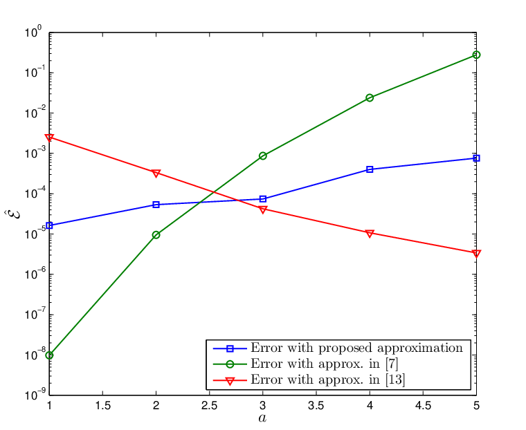
We next compare $\hat{\mathcal{E}}$ for our proposed approximation and the one given in [7, 13]. Results shown in Fig. 4 for different values of $a$ demonstrate the accuracy of the proposed scheme. As mentioned in the previous section, the range of $a$ values considered in the plot is the range that would typically be encountered in practice in communication system analysis with Rician fading [10]. However, for the problem defined in (5), it is guaranteed that the solution would minimize the error term for any value of $a$ .

V Conclusion

In this paper, a simple approximation of the first order Marcum $Q$ -function was presented that can be used in network connectivity analysis. For small input argument $a$ , an analytical approach was presented for finding the approximation parameters, while for larger $a$ , a numerical procedure based on an optimization problem was proposed. Equations for approximating these parameters were then presented. Simulation results demonstrated that the approximations led to an accurate representation of the Marcum $Q$ -function, especially for small values of $b$ . As $b$ tends to infinity however, existing bounds of $Q_{1}(a,b)$ yield to a closer representation of the function.

Acknowledgement

The authors would like thank Toshiba Telecommunications Research Laboratory and the EPSRC (grant EP/H500316/1) for their continued support.

References

[1] M. K. Simon and M.-S. Alouini, “Some New Results for Integrals Involving the Generalized Marcum Q- Function and their Application to Performance Evaluation over Fading Channels,” IEEE Trans. Wireless Commun., vol. 2, no. 4, pp. 611–615, 2003.
[2] C. O’driscoll and C. Murphy, “A Simplified Expression for the Probability of Error for Binary Multichannel Communications,” IEEE Trans. Commun., vol. 57, no. 1, pp. 32–35, 2009.
[3] H. Fu and P.-Y. Kam, “Exponential-Type Bounds on the First-Order Marcum Q-Function,” in Proc. IEEE Global Telecommunications Conf. (GLOBECOM 2011), 2011, pp. 1–5.
[4] X. Zhao, D. Gong, and Y. Li, “Tight Geometric Bound for Marcum Q-Function,” Electronics Letters, vol. 44, no. 5, pp. 340–341, 2008.
[5] M. K. Simon and M.-S. Alouini, “Exponential-Type Bounds on the Generalized Marcum Q-Function with Application to Error Probability Analysis Over Fading Channels,” IEEE Trans. Commun., vol. 48, no. 3, pp. 359–366, 2000.
[6] N. Ding and H. Zhang, “A Flexible Method to Approximate Marcum Q-Function Based on Geometric Way of Thinking,” in Proc. 3rd Int. Symp. Communications, Control and Signal Processing ISCCSP 2008, 2008, pp. 1351–1356.
[7] P. C. Sofotasios and S. Freear, “Novel Expressions for the Marcum and One Dimensional Q-Functions,” in Proc. 7th Int Wireless Communication Systems (ISWCS) Symp, 2010, pp. 736–740.
[8] B. Ake, Numerical Methods for Least Squares Problems. Society for Industrial and Applied Mathematics, 1996. [Online]. Available: http://epubs.siam.org/doi/abs/10.1137/1.9781611971484
[9] A. R. Luxmoore, “Statistical Methods for Engineers and Scientists,” International Journal for Numerical Methods in Engineering, vol. 14, no. 2, pp. 313–313, 1979. [Online]. Available: http://dx.doi.org/10.1002/nme.1620140217
[10] J. Proakis, Digital Communications, 4th ed. McGraw-Hill Higher Education, Sept 2000, iSBN-13: 978-0072321111.
[11] D. Miorandi, “The Impact of Channel Randomness on Coverage and Connectivity of Ad Hoc and Sensor Networks,” IEEE Trans. Wireless Commun., vol. 7, no. 3, pp. 1062–1072, 2008.
[12] J. Coon, C. P. Dettmann, and O. Georgiou, “Full Connectivity: Corners, Edges and Faces,” Journal of Statistical Physics, vol. 147, pp. 758–778, 2012. [Online]. Available: http://dx.doi.org/10.1007/s10955-012-0493-y
[13] R. Li, P. Y. Kam, and H. Fu, “New Representations and Bounds for the Generalized Marcum Q-Function via a Geometric Approach, and an Application,” IEEE Trans. Commun., vol. 58, no. 1, pp. 157–169, 2010.
[14] M. Pent, “Orthogonal polynomial approach for the marcum qfunction numerical computation,” Electronics Letters, vol. 4, no. 25, pp. 563 –564, 13 1968.

An Approximation of the First Order Marcum QQ-Function with Application to Network Connectivity Analysis