Community Structure Detection in Complex Networks with Partial Background Information

In many real applications, we often have some background information that can be used for community structure detection. Specifically, we consider the following two types of pairwise constraints:

• 1.

  Must-Link constraints $C_{ML}$: $(i,j)\in C_{ML}$ means that the two nodes $i$ and $j$ must belong to the same community,

• 2.

  Cannot-Link constraints $C_{CL}$: $(i,j)\in C_{CL}$ means that the two nodes $i$ and $j$ cannot belong to the same community.

We incorporate the constraints $C_{ML}$ and $C_{CL}$ into the adjacency matrix $A^{[1]}$ to get a new matrix $B$ as follows:

where $\alpha$ is a positive constant.

As one can see, if we set $\alpha$ to 1, and for all the pairs of nodes, we know whether they should belong to $C_{ML}$ or $C_{CL}$, or in other words, we know very well the community structures in the graph, the adjacency matrix will reduce to the standard consensus matrix, whose $(i,j)th$ element means whether node $i$ and node $j$ are in the same community, $1$ means yes and $0$ means no. Hence from the viewpoint of consensus matrix, incorporating prior knowledge can be regarded as the de-noising process.

We have tried different $\alpha$, i.e., $\alpha=1$ and $\alpha=2$, and the results of $\alpha=2$ always get better. We omit the comparisons here due to space limit.

After incorporating background information into the adjacency matrix, we then apply nonnegative matrix factorization (NMF), spectral clustering and InfoMap, which are of the most common and widely-used models in unsupervised learning, for community structure detection.

NMF can be expressed as follows: given a nonnegative objective matrix $X$ of size $n\times m,$ columns of which are samples and rows are features, we try to find two nonnegative matrices $F$ of size $n\times k$ and $G$ of size $m\times k$ such that: $X\approx FG^{T}.$ This problem is often formulated as the following nonlinear programming:

where $J(X\|FG^{T})$ is the cost function that measures the dissimilarity between $X$ and $FG^{T}$, and $\geqslant 0$ means that $F$ and $G$ should not have negative entries. The most popular algorithm designed for NMF is multiplicative update rules. The objective matrix $X$ for NMF can be selected as $B$.

In [6], it showed that the diffusion-kernel-based similarity matrix $SK$¹¹ 1 Definition of diffusion kernel $K$ and the similarity matrix $SK$ [6, 7]: $K=\lim\limits_{n\to\infty}(1+\displaystyle\frac{\beta L}{n})^{n}=expm(\beta L)$, where $L$ is the opposite Laplacian of $A^{[0]}$: $$L_{ij}=\left\{\begin{array}[]{rcl}\vskip 2.84526pt1&&\mbox{if}\ i\sim j\\ \vskip 2.84526pt-d_{i}&&\mbox{if}\ i=j\\ 0&&\mbox{otherwise,}\end{array}\right.$$ and $d_{i}$ is the degree of node $i$. $$SK_{ij}=\frac{K_{ij}}{\sqrt{K_{ii}K_{jj}}}.$$ We set $\beta=0.2$ in this paper. Note that there is a MATLAB command “expm” for the exponential of a matrix. was the best choice for the objective matrix $X$ among all the candidates, hence we also tested the performance of $SK$ in this paper.

The community structures of the network can be obtained from $G$: node $i$ is of community $k$ if $G_{ik}$ is the largest element in the $i$th row of $G$.

1. 1)

   Standard NMF with least squares error: If $J(X\|FG^{T})$ is selected as the least squares error: $J(X\|FG^{T})=\|X-FG^{T}\|_{F}^{2}$, the algorithm of multiplicative update rules can be summarized in Algorithm 1. In this paper, the iteration number iter is set to 100.                

   0:  $X,$ iter

   0:  $F,G.$

   1:  for $t=1:\mbox{iter}$ do

   2:   $\displaystyle F_{ik}:=F_{ik}\frac{(XG)_{ik}}{(FG^{T}G)_{ik}}$

   3:   $\displaystyle G_{ik}:=G_{ik}\frac{(X^{T}F)_{ik}}{(GF^{T}F)_{ik}}$

   4:  end for

2. 2)

   Standard NMF with K-L divergence: If $J(X\|FG^{T})$ is selected as the KL divergence: $\displaystyle J(X\|FG^{T})=\sum_{i,j}[X_{ij}\log\frac{X_{ij}}{(FG^{T})_{ij}}-X_{ij}+(FG^{T})_{ij}],$ the corresponding update rules of $F$ and $G$ are:

   $$\displaystyle F_{ik}:=\frac{F_{ik}}{\sum_{j}G_{jk}}\sum_{j}\frac{X_{ij}}{(FG)_{ij}}G_{jk};$$

   $$\displaystyle G_{jk}:=\frac{G_{jk}}{\sum_{i}F_{ik}}\sum_{i}\frac{X_{ij}}{(FG)_{ij}}F_{ik}.$$

3. 3)

   Symmetric NMF (SNMF): There is a variant of NMF for semi-supervised clustering, whose objective function can be formulated as: $\|X-GSG^{T}\|_{F}^{2}$. The update rules of $G$ and $S$ are [5]:

   $$G_{ik}:=G_{ik}\frac{(XGS)_{ik}}{(GSG^{T}GS)_{ik}};$$

   $$S_{ik}:=S_{ik}\frac{(G^{T}XG)_{ik}}{(G^{T}GSG^{T}G)_{ik}}.$$

4. 4)

   Bayesian NMF [8]: It optimizes the NMF model under the Bayesian framework, and can get better results under some circumstances.

Spectral clustering is very powerful in its simplicity and effectiveness, which can be summarized in Algorithm 2. Note that there are many variations of the standard one, and the detailed analysis can be found in [10, 11].

This model grew out of information theory, and tries to reveal the communities by optimizing a quality function about the minimum description length of random walks on the network. The model is among the best for community detection [13].

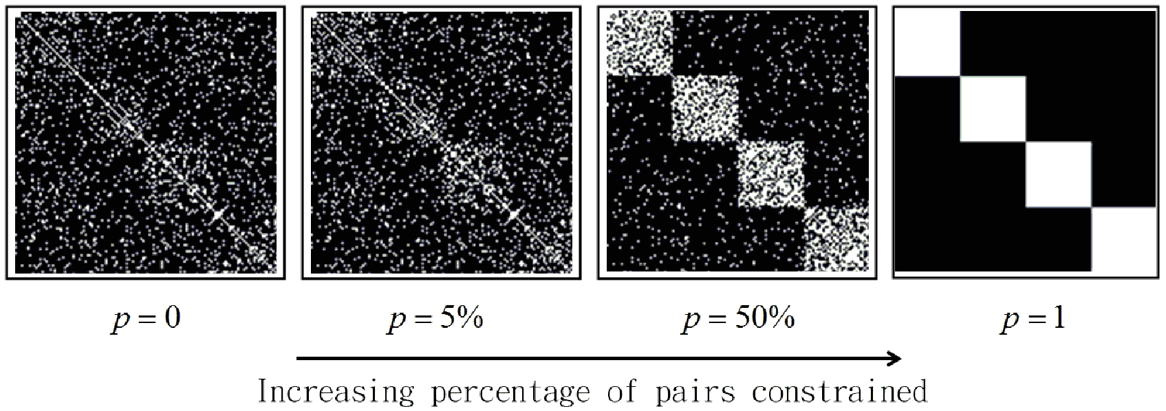
We close this section by an illustrative example as follows: we try to detect the community structures in a GN network with 128 nodes (For details, see Data Description, $Zout=10.$). The network has 4 communities with 32 nodes each. The heatmap of the corresponding adjacency matrix $A^{[1]}$ is shown as the leftmost in Fig. 1. If we have prior knowledge about the network structure so that we can determine a percentage of pairs of nodes as must-link or cannot-link, we can incorporate them into $A^{[1]}$. As one can see in Fig. 1, the adjacency matrix becomes more and more clear as the percentage of pairs constrained increases, and finally reduces to the standard consensus matrix of the community structures. This example demonstrates that background information is valuable to improve the accuracy of community structure detection.

We used both synthetic and real-world networks to test the effectiveness of our methods. The details of these datasets are as follows:

1. 1)

   GN [1] : Maybe the most widely used benchmarks are GN networks. The network has $128$ nodes which are divided into four non-overlapping communities with $32$ nodes each. The degree of each node is $Zin+Zout=16$, in other words, each node averagely has exactly $16$ edges which randomly connect $Zin$ nodes in its own community and $Zout$ nodes in other communities. As one can see, with the increasing $Zout$, the community structures will become less clear and the problem more challenging. In this paper, we set $Zout$ to 8.

2. 2)

   LFR [14] : Indeed, in most of the real applications, the community structures are more complicated than GN networks. The size of the network might be larger, or the numbers of the nodes in different communities might not be identical, or different nodes might have different positions, i.e., some are ¡°superstars¡± or ¡°hubs¡± and should have higher degrees while the others are leaves. The LFR benchmark networks are thus proposed to address these problems. In LFR networks, both the degree and the community size distributions are power laws, with exponents $\gamma$ and $\beta$, which is more practical. Each node has a fraction $1-\mu$ of its links with the nodes in its own community and a fraction $\mu$ with the other ones. Here $\mu$ is called the mixing parameter.

   We set the parameters of the LFR network as follows: the number of nodes was $1000$, the average degree of the nodes was $20$, the maximum degree was $50$, the exponent of the degree distribution $\gamma$ was 2 and that of the community size distribution $\beta$ was 1, and the mixing parameter $\mu$ was $0.8$. The communities were non-overlapping.

3. 3)

   Karate [15]: this dataset contains the network of friendships between 34 members of a karate club at an American university. This club was by chance split into two smaller ones due to the divergence of opinions about the club fees.

4. 4)

   Football [1]: this dataset contains the network of American football games (not soccer) between Division IA colleges during regular season Fall 2000. There are 115 nodes representing the football teams while an edge means there was a game between the teams connected by the edge. The teams were divided into 12 conferences, and all teams except few (mainly in two conferences) played against the ones in the same conference more frequently than those in other conferences.

In our experiments, the normalized mutual information (NMI, [16]) was used as the standard to evaluate the community structure detection performance. The value can be formulated as follows:

where $M_{1}$ is the ground-truth cluster label and $M_{2}$ is the computed cluster label, $k$ is the community number, $n$ is the number of nodes, $n_{ij}$ is the number of nodes in the ground-truth cluster $i$ that are assigned to the computed cluster $j$, $n_{i}^{(1)}$ is the number of nodes in the ground-truth cluster $i$ and $n_{j}^{(2)}$ is the number of nodes in the computed cluster $j$, $\log$ is the natural logarithm.

Compared with simply counting the number of misclassified nodes, NMI is more informative, especially suitable for imbalanced datasets (i.e., the numbers of the nodes in different communities are not identical). For example, in a four-sample toy data, the ground-truth cluster label could be $1,1,1,2$. The computed cluster labels of two different models were $1,1,1,1$ and $1,1,2,2$ respectively. In other words, the smaller cluster was masked and not detected by the first model, hence the second model should be better though it also had one sample mis-clustered. But the accuracy (number of misclassified nodes divided by the number of nodes in the graph) results of these two models were all $75\%$, which was misleading. On the other hand, the NMI under this case was $0$ (the numerator of NMI was: $3\log\displaystyle\frac{3\cdot 4}{3\cdot 4}+1\cdot\log\displaystyle\frac{1\cdot 4}{1\cdot 4}=0$) and $34.56\%$ respectively, which was relatively more reasonable and informative.

In the case study, we also used the modularity function $Q$ [17, 18] as the standard to determine the best community number $k$. The function can be defined as follows:

where $C_{k}$ is the $k$th community in the graph, $L(V_{1},V_{2})=\sum\limits_{i\in V_{1},j\in V_{2},i\neq j}a_{ij},$ and $a_{ij}$ is the element of $A^{[0]}.$

The larger the values of NMI and Q, the better the graph partitioning results.

Firstly, we compared the clustering performance of NMF-based models with different similarity measures including $A^{[0]}$, $A^{[1]}$, $C^{[A]}$ and $SK$. The results show that $A^{[1]}$ is a competitive one, though there is no single winner. Note that calculating the diffusion kernel is time consuming for large scale networks, hence we used $A^{[1]}$ for the NMF-based models in the following experiments. The details are omitted here due to space limit.

In this subsection, we systematically compared the results of NMI obtained by the models on the artificial datasets and the karate network with prior knowledge available. For an undirected network with $n$ nodes, there are totally $n(n-1)/2$ node pairs available. We randomly picked out some pairs of nodes, and determined whether they belonged to $C_{ML}$ or $C_{CL}$: if the two nodes had the same community label, they were must-link, otherwise, they were cannot-link. The results were averages of ten trails and given in Fig. 2 and Table 1. From these figure and table, one can observe that: i) The trends of all the models are generally identical and the values of the averaged NMI increase with the increasing percentage of pairs constrained; ii) for synthetic datasets: GN and LFR, the model of InfoMap and the spectral clustering are better than the NMF-based models, especially for the LFR datasets; iii) for the karate network, NMF with least squares error performs better; iv) our proposed framework is flexible and model independent, or in other words, it can be naturally combined with many models, such as NMF, spectral clustering, InfoMap, etc.

In summary, our proposed semi-supervised framework does greatly enhance the results of community structure detection by benefitting from the user provided background information.

In this subsection, we used the college football network for a case study, and saw the partitioning results of NMF_LSE given different percentages of pairs constrained. Actually, we also tried spectral clustering and got similar results. Details of spectral clustering are omitted here due to space limit.

The teams were separated into 12 conferences, and most of them played against the ones in the same conference more frequently. However, the teams 37, 43, 81, 83, 91 (in conference IA Independents), 12, 25, 51, 60, 64, 70, 98 (in conference Sunbelt), 111, 29 and 59 played more frequently against the ones in other conferences. Table 2 lists the basic information about these teams, from which one can observe that three out of five teams in IA Independents never played against the ones in the same conference and the other two teams played only once.

Firstly, we tried to determine the community number $k$. We compared the values of modularity $Q$ at different $k$, and the function achieved its peak value at $k=11$. By combining the results of $Q$ values in Table 3 with the information in Table 2, we set the community number $k=11$ and the teams in IA Independents would be assigned to the other eleven conferences based on the outputs of NMF. Hence there were $115-5=110$ teams with ground-truth conference labels and totally $110\times(110-1)/2=5995$ team pairs available. We randomly selected some pairs as constraints: if the two teams of the pair were in the same conference, they were must-link (ML), otherwise, they were cannot-link (CL).

Figure 3 gives the resulting partitions of NMF corresponding to different percentages of pairs constrained. When given no prior knowledge constrained, there were $5$ abnormal teams mis-clustered: teams 29, 60, 64, 98, 111; But after randomly given $5$ percent of pairs constrained, the results were significantly improved and only two abnormal teams were mis-clustered: teams 29 and 111. Finally, when given $20$ percent, there was only one team mis-clustered: team 59. From these results, one can see that: 1) NMF is really good enough in that only some abnormal teams are not correctly clustered; 2) our semi-supervised clustering framework does take the background information and domain knowledge into consideration, which makes the partitioning results more explainable.

Finally, we ask an interesting question: how to select the prior information and incorporate them into the models? To the best of our knowledge, in practice, the most widely used method is to randomly select some pairs of samples or nodes and manually determine whether they are must-link or cannot-link based on the domain knowledge. But are there any better methods to select the pairs that can either reduce the workload or improve the clustering performance, or both? Indeed, for a large scale network, a very small percentage of pairs may still mean a huge workload. In this subsection, we attempted to introduce a new rule-based method to address this problem. Firstly, we computed the hamming distances between all pairs of nodes (rows of $A^{[1]}$), and sorted the distances to find the largest and the smallest ones (this step can be finished by programming calculation, not manually). We selected the pairs that have the largest distances and the smallest distances simultaneously. For example, if we wanted to select $P$ pairs of nodes, we selected $P/2$ pairs with the largest distances, and also selected $P/2$ pairs with the smallest distances. Then we manually decided whether the selected pairs were must-link or cannot-link and incorporated them into the clustering process. The results on GN datasets are shown in Fig. 4, from which one can observe that our preliminary results are not good enough compared with that of randomly based. Hence we leave the problem open and believe that it deserves further study.

References

- [1] M. Girvan, M. E. J. Newman, Proceedings of the National Academy of Sciences 99 (12) (2002) 7821–7826.
- [2] X. Wu, Z. Liu, Physica A 387 (2008) 623–630.
- [3] D. D. Lee, H. S. Seung, Nature 401 (6755) (1999) 788–791.
- [4] D. D. Lee, H. S. Seung, NIPS, 2000, pp. 556–562.
- [5] Y. Chen, M. Rege, M. Dong, J. Hua, Seventh IEEE International Conference on, IEEE, 2007, pp. 103–112.
- [6] R. Wang, S. Zhang, Y. Wang, X. Zhang, L. Chen, Neurocomputing 72 (2008) 134–141.
- [7] R. I. Kondor, J. Lafferty, in: International Conference on Machine Learning (ICML), 2002, pp. 315–322.
- [8] I. Psorakis, S. Roberts, M. Ebden, B. Sheldon, Physical Review E 83 (6) (2011) 066114.
- [9] A. Ng, M. Jordan, Y. Weiss, Advances in neural information processing systems 2 (2002) 849–856.
- [10] H. Shen, X. Cheng, Journal of Statistical Mechanics: Theory and Experiment 2010 (2010) P10020.
- [11] X. Ma, L. Gao, Journal of Statistical Mechanics: Theory and Experiment 2011 (2011) P05012.
- [12] M. Rosvall, C. Bergstrom, Proceedings of the National Academy of Sciences 105 (4) (2008) 1118–1123.
- [13] A. Lancichinetti, S. Fortunato, Physical Review E 80 (5) (2009) 056117.
- [14] A. Lancichinetti, S. Fortunato, F. Radicchi, Phys. Rev. E 78 (2008) 046110.
- [15] W. W. Zachary, Journal of Anthropological Research 33 (1977) 452–473.
- [16] A. Strehl, J. Ghosh, Journal of Machine Learning Research 3 (2002) 583–617.
- [17] M. Newman, M. Girvan, Physical review E 69 (2) (2004) 026113.
- [18] M. Newman, Proceedings of the National Academy of Sciences 103 (23) (2006) 8577–8582.
- [19] X. Ma, L. Gao, X. Yong, L. Fu, Physica A: Statistical Mechanics and its Applications 389 (1) (2010) 187–197.