Conserved actions, maximum entropy and dark matter halos
Abstract
We use maximum entropy arguments to derive the phase space distribution of a virialized dark matter halo. Our distribution function gives an improved representation of the end product of violent relaxation. This is achieved by incorporating physically motivated dynamical constraints (specifically on orbital actions) which prevent arbitrary redistribution of energy.
We compare the predictions with three high-resolution dark matter simulations of widely varying mass. The numerical distribution function is accurately predicted by our argument, producing an excellent match for the vast majority of particles.
The remaining particles constitute the central cusp of the halo ( of the dark matter). They can be accounted for within the presented framework once the short dynamical timescales of the centre are taken into account.
1 Introduction
For over two decades it has been possible to use numerical methods to model systems of cold, collisionless dark matter particles collapsing under gravity to form stable, virialized ‘halos’ (Frenk et al. 1985; Dubinski & Carlberg 1991; for a review see Frenk & White 2012). The density of these halos declines with radius following a slowly changing power law dependence, roughly at small radii and in the outer regions (Navarro et al., 1996b; Kravtsov et al., 1997; Moore et al., 1998). Despite some early uncertainty, recent simulations with independent computer codes all reproduce this result (Diemand et al., 2008; Navarro et al., 2010; Stadel et al., 2009, e.g.). The universal behaviour seems to be independent of the power spectrum of initial linear density fluctuations (Moore et al., 1999; Reed et al., 2005; Wang & White, 2009) as well as the mass of the collapsed object and the epoch of collapse, although together these determine a scale radius for the transition from to behaviour (Cole & Lacey, 1996; Navarro et al., 1997; Bullock et al., 2001b; Eke et al., 2001; Macciò et al., 2007). Even simulations of ‘cold collapse’, for which initial conditions consist of a homogeneous sphere of particles, seem to produce similar universal profiles (Huss et al., 1999).
It remains an outstanding question, however, whether this universality can be adequately explained from first principles. Until this question is answered, we do not fully understand what the universality means and must rely on new simulations to predict the effect of changes in the initial conditions or particle properties. The experimental result that monolithic collapse produces the same types of system as hierarchical merging (Huss et al., 1999; Moore et al., 1999; Wang & White, 2009) is provocative: it means that any explanation for universality which invokes a specific cosmology (Syer & White, 1998; Dekel et al., 2003; Salvador-Solé et al., 2012, e.g.) must be describing a special case of a more general process (Manrique et al., 2003).
Attempts to understand collisionless gravitational collapse’s insensitivity to initial conditions were pioneered by Lynden-Bell (1967) in the context of self-gravitating stellar systems. Adopting Boltzmann’s procedure for deriving the thermodynamics of collisional systems, Lynden-Bell maximized the entropy of the systems subject to fixed energy. This implies a density profile obeying , so disagrees with the results of numerical experiments. Moreover this approach gives rise to a number of physically questionable conclusions (Padmanabhan, 1990; Lynden-Bell, 1999, for reviews see). The clearest of these is the ‘gravothermal catastrophe’: entropy can be increased without bound by transferring energy from the innermost orbits of a self-gravitating system to the outermost orbits (Lynden-Bell & Wood, 1968; Tremaine et al., 1986). This implies the existence of a runaway physical instability in which the majority of material collapses into an extreme central density cusp or black hole.
Observations and numerics both suggest that something prevents the above catastrophe from occurring on any reasonable timescale; in other words, a physical constraint is preventing the arbitrary redistribution of energy (White & Narayan, 1987). In the spirit of Jaynes (1957) a general explanation for the final state can still be based on the ideas of statistical mechanics but in the presence of constraints other than energy. The additional constraints will represent the incompleteness of the energy equilibriation effects of violent relaxation.
This is the approach we adopt in the present work. The likely distribution of particles in phase space is selected by maximizing entropy,
| (1) |
where is Boltzmann’s constant and is the probability of finding a particle in a specified region of phase space , subject to relevant constraints on the desired solution. (This approach can be motivated by showing that the vast majority of states consistent with a given set of constraints are to be found near the maximum entropy solution; see Appendix A for further discussion and references.)
The constraints applied arise from the dynamical evolution of collisionless systems. We will argue that, in the late stages of violent relaxation, there is a diffusion of particles in phase space which approximately conserves the sum of orbital actions. This sum is progressively better conserved as equilibrium is approached and therefore its role in establishing that equilibrium cannot be ignored. Applying the maximum entropy recipe, we will show that the phase space structure of equilibrium halos is then reproduced over orders of magnitude in probability density. To our knowledge, this is the first instance of maximum entropy reasoning, applied to 6D phase space and subject to physically motivated constraints, producing such success in a collisionless system.
The remainder of this work is organized as follows. First, the conservation of action is discussed (Section 2.1). Then a canonical ensemble constructed on this basis (Section 2.2) yields a phase space distribution in quantitative agreement with high resolution numerical experiments (Section 3). A discrepancy affecting a small fraction of particles at low angular momentum is highlighted in Section 3.3. Finally we discuss the predicted radial density profiles which again highlight the need for special treatment of low angular momentum orbits (Section 3.5). We conclude in Section 4.
2 The analytic phase space distribution
2.1 Conservation of action
Our first task is to identify and explain some relevant quantities which should be held fixed when maximizing entropy. This will be central to our argument because such constraints represent the incompleteness of violent relaxation’s tendency to redistribute energy, generating a different solution from the one based on energy conservation alone. With this in mind we will show that the radial action (to be defined below) is conserved in an average sense even during rapid potential changes.
This average conservation does not appear to have been discussed elsewhere in the literature. We will first show how it can be derived from previous work (Pontzen & Governato, 2012) when the potential changes instantaneously, maintaining the sphericity of the halo. Then a more general (but more abstract) argument will be given which additionally shows that the other two actions (the -component of the angular momentum and the scalar angular momentum ) are also conserved in the same average sense. The second approach encompasses perturbations to the potential which have variations on arbitrary timescales and may break spherical symmetry. However the first has a more intuitive content and therefore forms our starting point.
In a spherical system, the radial action is defined by
| (2) |
Here is the specific energy, is the specific angular momentum and is the potential at a given radius and time ; the integral is taken over the region where the integrand is real.
The radial action has the same units as specific angular momentum . This reflects the similar conservation roles these two quantities play for the radial and angular components of the motion. In particular is exactly conserved if any changes in the potential occur sufficiently slowly (‘adiabatically’) in time (Binney & Tremaine, 1987, e.g.).
On the other hand in the rapid, impulsive limit under an instantaneous change in energy and potential , the action of the particle is changed at first order:
| (3) |
In Pontzen & Governato (2012) we showed that the energy shift induced by the change of potential, averaged over possible orbital phases of the particle, is
| (4) |
an exact result (Pontzen & Governato, 2012, see equation 12 of). Here angular brackets denote averaging over all possible phases of the orbit. Considering the probability distribution of radial actions after this change, one has at first order, by substituting equation (4) in (3). Even though a specific particle will change its radial action, the ensemble average is conserved.
This result connects closely with the standard adiabatic argument that if any changes to the potential occur on long timescales. In our case, however, the necessary ‘phase averaging’ does not occur over time for an individual particle but instead via a statistical consideration of an ensemble of particles spread evenly through all possible phases.
We can generalize as follows. Adopting the complete set of action-angle coordinates for phase space (Park, 1990; Binney & Tremaine, 1987, e.g.), the momenta are where is the total angular momentum and is its component in the direction (so ). The conjugate coordinates are , taken to be periodic with interval , and the Hamiltonian is
| (5) |
Here is an arbitrary perturbation. It may consist of a long-lived term (perhaps a departure from spherical symmetry) and fluctuations on arbitrary time-scales. In the background, the coordinates change at a constant rate,
| (6) |
and the frequencies for the radial and azimuthal motion and obey
| (7) |
by Hamilton’s equations. The frequencies may change slowly with time (). is conserved in the background but when is non-zero, the equations of motion read
| (8) |
Because equation (6) shows that particles in the background move at a uniform rate in the coordinates, an equilibrium distribution has no dependence; i.e. the density is a function of alone11 1 The conjugate coordinate to is also a constant of motion in the background, so this argument does not strictly show . However must be exactly conserved anyway if the perturbations are internally generated, since it is proportional to a component of the total angular momentum vector.. From this it follows that
| (9) |
where the result is obtained via integration by parts. This means an individual particle’s can ‘diffuse’ (Binney & Lacey, 1988) over large distances in action space,
| (10) |
compared to the variation in the mean of the population,
| (11) |
We can inspect this diffusion in a simulation by calculating the relevant actions at two timesteps. As an example, Figure 1 shows a histogram of changes in the radial action of tightly bound particles in the forming “Dwarf” halo (see Section 3) between and , a time interval of approximately . We define ‘tightly bound’ by selecting particles interior to at the earlier time step, and calculate the values of these particles in both outputs according to the numerical recipes given later (Section 3.1).
As expected from the linear analysis, Figure 1 shows that individual simulated particles change their actions more rapidly than the population mean. Quantitatively, the change in the population mean is whereas a typical particle has moved by from its original value. Note also that the mean value for these particles in the final timestep is , meaning particles really do cover significant distances in action space.
This analysis confirms that evolves slowly and, although it is not exactly conserved, it forms a constraint of motion that cannot be ignored on finite timescales. A complete description would require investigation of different moments of the distribution at higher order in perturbation theory. For now, however, we have motivated a picture in which evolves sufficiently slowly compared to the diffusion of an individual particle that it must be considered fixed in analysis of the distribution.
2.2 The new canonical ensemble
In the Introduction we explained that, to obtain a phase space distribution function, we will maximize the entropy (1) subject to constraints on the particle population (further discussion is given in Appendix A). As well as energy conservation, we apply the 3-vector of constraints on discussed above. This gives rise to a total of four Lagrange multipliers in the resulting distribution function:
| (12) |
where the Lagrange multipliers are and . In the absence of the new constraints, and is identified with (where is the thermodynamical temperature).
All four constants can be determined in a variety of ways depending on the situation; for a complete account of structure formation one would like to be able to derive them from the initial conditions, but this lies beyond the scope of the current paper (although see Section 3.4 for further comments). The lack of any reference to in equation (12) indicates that the solution is phase-mixed, as required for equilibrium.
Equation (12) is the essential prediction of the present work. As with any prediction derived from a maximum entropy argument, it will be able to fit the actual ensemble only if we have encapsulated enough of the dynamics within the constraints (Jaynes, 1979b). The rest of this paper is concerned with testing to what extent that is the case.
| Dwarf | MW | Cluster |
| ; ; | ; ; | ; ; |
| ; . | ; . | ; . |
First consider the probability of finding a particle with in a given interval (ignoring and coordinates). This is given by
| (13) |
because the action-angle coordinates are canonical, so the phase-space measure is constant. In the limit that the energy of the system becomes large at fixed action, equation (13) can be solved:
| (14) |
but it is not immediately clear whether we will be operating in this regime. More generally a closed form for is hard to obtain, but we can at least show that
| (15) |
which can then be integrated numerically for a given case to give a concrete comparison between equation (12) and simulations. Here we have defined
| (16) |
which is the mean of the radial frequency for particles with a fixed . With this definition, relation (15) can be derived from equation (13), recalling that the radial frequency of the particle’s orbit obeys equation (7). We will investigate and explain the distribution of values predicted by equation (15) in Section 3.2.
Now consider the distribution of total angular momentum . We will follow exactly the same series of manipulations as for the radial action; however in this case the marginalization over introduces a non-trivial term:
| (17) |
Once again, in the case , we have a fully analytic expression for ,
| (18) |
which will serve as a useful point of comparison. More generally we can differentiate equation (17) to obtain
| (19) |
where is the angular frequency of the orbit and
| (20) |
is the mean angular frequency of particles at fixed . Equation (19) for the angular momentum distribution (ignoring all other coordinates) is the equivalent of equation (15) for the radial action distribution. Once again we will investigate and explain the shape it predicts in Section 3.3. First, however, we will explain the simulations which serve as a point of comparison for the later discussions.
3 Comparison to simulations
3.1 Overview of the simulations
In the previous section we applied maximum entropy reasoning to conservation of energy and approximate conservation of action to derive an expected equilibrium phase space distribution. We will now compare that expectation against simulated dark matter halos. Our strategy is to integrate equations (15) and (19) numerically for these simulations and compare to the actual distribution of particles binned by and respectively.
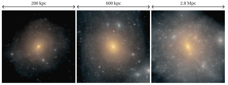
We will present results from three simulated dark matter halos (shown in Figure 2), chosen to span a wide range of masses with an approximately constant number of particles per halo (several million in each case). We also compared our results against the GHALO multi-billion-particle phase space (Stadel et al., 2009), finding good agreement similar to that described for our “MW” halo here. This gives confidence that the mechanisms and results discussed in the paper are not sensitive to numerical resolution.
Our simulations are run from cosmological initial conditions at in a ‘zoom’ configuration (Navarro & White, 1993), i.e. with high resolution for the main halo and its immediate surroundings and lower resolution for the cosmological environment. The softening lengths for the high resolution region are listed in Figure 2 and are fixed in physical units from , prior to which they scale linearly with cosmological scalefactor, a compromise motivated by numerical convergence studies (Diemand et al., 2004). We verified at the final output () that the high resolution regions have not been contaminated by low resolution particles, and that the halo real-space density profiles are well described by a slowly rolling powerlaw, in accordance with all recent simulations (e.g. Diemand et al., 2008; Stadel et al., 2009; Navarro et al., 2010, and references therein).
Each simulation output contains full cartesian phase space coordinates (, ). The position space is re-centred on the central density peak of the halo using the ‘shrinking sphere’ method of Power et al. (2003). The velocities are re-centred such that a central sphere of radius has zero net velocity, where is the radius at which the mean halo density is times the critical density. Henceforth we only consider particles inside .
From left to right in Figure 2 the simulated halos become more massive. The width of each panel is equal to and the luminosity is scaled to represent the column density over a dynamic range of . The most conspicuous aspect of Figure 2 is that the halos become less centrally concentrated. We verified this by fitting a classic “NFW” (Navarro et al., 1996b) formula to the density profile. The NFW fit,
| (21) |
yields , a characteristic density, and , a scale radius. The latter is often expressed in a scale-free manner as a concentration value ; we have recorded the value for each halo in Figure 2. As expected the concentration decreases with increasing mass, in agreement with previously known trends (Macciò et al., 2007; Bullock et al., 2001b, e.g.). We thus have a sample of cosmological halos which span a wide range in both mass and concentration. These different concentrations are thought to arise from different mean densities in the universe at the epoch of collapse (Navarro et al., 1997; Bullock et al., 2001b).
All halos in Figure 2 exhibits large amounts of substructure; we will present results with this substructure subtracted, although we have verified that including the substructure does not have a qualitative impact on our results. The substructure is identified and removed using the “Amiga Halo Finder” (Knollmann & Knebe, 2009). For each remaining particle inside , the specific scalar angular momentum is given by . We calculate by evaluating equation (2) numerically, using a spherically-averaged potential defined by
| (22) |
where is the total mass enclosed by a sphere of radius , and the specific energy of each particle is defined as . is evaluated using the true spherical potential out to , beyond which (for reasons of numerical speed) the calculation is truncated and an analytic completion assuming a Keplerian (vacuum) potential is taken. We verified that changing to had little impact on the results.
Before proceeding to a comparison, we need to derive appropriate values. We calculate these using a Monte-Carlo Markov chain (MCMC) to maximize the likelihood
| (23) |
where is the 1-particle distribution function (12) normalized such that . This normalization must be accomplished numerically on a grid of values; at each grid-point is calculated by operating a bisection search on equation (2). This need only be done once, and then the evaluation of each link in the Markov chain is rapid.
The operation gives us maximum likelihood (i.e. ‘‘best fit’’) parameters22 2 The MCMC technique also yields uncertainties on the values, but these will not be considered further in the present work. for a given simulation, optionally subject to constraints (such as or ). We are now fitting up to four parameters (excluding mass normalization), more than the one or two parameters normally used by simulators to describe their halos (Navarro et al., 2004; Stadel et al., 2009, e.g.). However the fitted real-space density profiles are purely phenomenological constructs; conversely here we are starting with a functional form derivable from physical considerations. As we have commented in Section 2.2 and will expand upon in Section 3.4, the ’s should ultimately therefore be derived from initial conditions. For the present, however, the objective is to see whether our physical argument can correctly describe the phase space distribution at all, for which fitting ’s is the most pragmatic approach.
3.2 Comparison with MW: distribution
We will now start to test how closely equation (12) represents the distribution of particles in our simulations. We will investigate MW in some detail, before showing results for the other two simulations to which the same discussion can essentially be applied.
The distribution of values in MW is shown by the histogram in the left panel of Figure 3. This can be compared with the thick solid curve which shows the distribution of values according to expression (15); the parameters are and . The agreement is excellent over several orders of magnitude in probability density, spanning the values where . Particles with account for less than of the mass and are on long period orbits, probably reflecting new material falling into the potential well. We will not consider them further.
The shape of the solution can be understood as follows. We have already remarked that, in the limit , one recovers equation (14), an exact exponential (i.e. a straight line on the linear-log axes of Figure 3). For comparison we have plotted the best fit distribution of this form (with ) as a dashed line. Since the period of an orbit increases with its energy (or radial action), the mean frequency decreases for increasing . So, inspecting equation (15), there will always be a value above which becomes much smaller than . Looking again at the thick solid curve in Figure 3, the limiting solution at high is indeed a pure exponential as this reasoning would suggest. At small , however, the gradient of the solution is steeper because of the energy term.
Comparing the histogram, the thick solid curve and the dashed line in the left panel of Figure 3 thus leads us to the conclusion that conservation (dashed line) accounts rather well for the qualitative form of the distribution, with an important correction from conservation at low . Finally the dotted curve shows the best fit case with – i.e. the normal statistical mechanical result in the absence of other constraints – and provides a poor fit at all . In summary, the identification of the constraint has resulted in dramatic improvements in the match to simulations.
3.3 Comparison with MW: distribution
Now consider the right panel of Figure 3 which shows the distribution of scalar angular momentum for the particles in our MW simulation. Once again the simulated particles are shown by the histogram; the best fit maximum entropy solution (, with as quoted above) is shown by the thick solid curve. It again reproduces the correct qualitative behaviour up to , with only of the mass at . Although the angular momentum distribution has some fluctuations away from the predicted behaviour, the predictions remain nearly correct over two orders of magnitude in probability density. With the exception of a problem described below, we do not believe these fluctuations to be of particular importance beyond indicating the structure is not completely relaxed. In particular we will show later (Section 3.5) that these inhomogeneities can be ignored when reconstructing a density profile in real space. Certainly compared against a solution based on conservation alone, again shown by a dotted curve, our solution can be counted a success.
The basic shape of the predicted distribution can be understood in a similar way to the distribution explained above. Consider again the case where (so in effect the total energy is unconstrained); then the exact solution is given by equation (18). We can also take the isotropic limit, , giving
| (24) |
This is analogous to the radial action case (14), but with a degeneracy factor reflecting the increasing density of available states available as the angular momentum vector grows in size. The result is that the abundance of particles grows linearly with for and decays exponentially for .
In light of the above discussion, it is notable that the turnover from growth to decay in occurs at values much smaller than . There are two ways to accomplish this. The first is to create a highly anisotropic setup, , where is the smallest value of interest. This packs orbits as much as possible into a single plane, generating a large net angular momentum and destroying the approximate spherical symmetry33 3 We note in passing that, technically, distribution functions with net angular momentum can nonetheless generate spherical potentials (Lynden-Bell, 1960)., but effectively removing the degeneracy in altogether:
| (25) |
Because it is maximally anisotropic, this solution cannot reflect the simulations; however if we temporarily fit only values using the functional form (18), we are pushed towards this unphysical limit (dashed line, Figure 3, right panel; ).
Luckily this is not the only way to overcome the shrinking phase space at low . Equation (19) shows that if increases fast enough as it can overcome the degeneracy term. We have verified that in the full solution (thick solid line in Figure 4 right panel), this is the mechanism by which the turnover is pushed to low .
Focussing attention on the low- part of the distribution does, however, reveal a deficiency in our predictions. Figure 4 shows the distribution of orbits with . The dotted line shows the same maximum entropy fit depicted by the solid line in Figure 3. When the horizontal scale is expanded in this way, it becomes clear that the global fit undershoots the simulation values significantly at low . This appears to be a systematic feature of all simulations we have inspected (the three detailed here, GHALO, and various other lower resolution simulations which we used for testing purposes). It is possible to force a better fit by restricting the likelihood analysis to this region, but the global agreement is then considerably worse.
This suggests that the behaviour at low is marginally decoupled from that in the rest of phase space. This could arise from the wide range of orbital periods: particles with small actions also have periods much shorter than the rest of the halo. The coupling between particles will necessarily be weak if their timescales are very different (since particles on short orbits react adiabatically to fluctuations on long timescales). This can substantially suppress redistribution of scalar angular momentum and is consistent with, although not reliant on, the early formation of a stable central cusp in simulations (Moore et al., 1998; Lu et al., 2006; Wang et al., 2011, e.g.).
In principle this weakness of coupling between orbits in different regions could be expressed as a further constraint in the maximum entropy formalism. Further investigation awaits future work, but for now we will use this as a motivation to study a two-population system. We are not suggesting that there really are two sharply defined populations, but that this should anticipate the features of incomplete equilibrium.
Our maximum likelihood analysis is able to find a dramatically better fit in this case, placing 3.5% of the mass in a second population at substantially lower temperature (). The summed distribution is shown by the thick solid line in Figure 4, with the contribution from the subdominant population indicated by the dashed line. Because the second distribution is so peaked near , the only difference at high is a marginal renormalization. We also verified that the distribution is barely affected.
It is undeniably disappointing that our solution does not automatically accommodate the behaviour at very low , but we expect that future development of the ideas above can quantitatively account for the discrepancy. We consider other possible explanations in Section 4. However after focussing so much on one corner of phase space we should re-emphasize the major conclusion: the distribution over both and for 96% of the particles are remarkably well described by the maximum entropy expression (12).
3.4 Other simulations
We confirmed that these basic conclusions persist in other simulations. The top row of figures in Figure 5 shows results from the ‘dwarf’ simulation. The distribution (top left panel) again shows excellent agreement for , where . Only a tiny fraction of mass () lies beyond this point of breakdown. As with MW, the dwarf’s angular momentum distribution (top right panel) has more conspicuous fluctuations, but still roughly adheres to the maximum entropy solution up to , with around of mass lying beyond this point. We verified that at very low angular momenta there is again an overabundance of particles in the simulation, although in this case it accounts for less than of particles compared against the in MW. The parameters of the dwarf fit are and .
Considering the cluster simulation (lower row of Figure 5) gives similar results once again. This time the distribution as well as the distribution shows some notable fluctuations around the maximum entropy description. This may be because clusters assemble later (as we discussed in Section 3.1, this is reflected in the lower concentration value), so the system is dynamically young; however we have not explicitly looked at time dependence of these distributions. The parameters of the cluster fit are and with and of the mass in the unrelaxed components beyond and respectively.
Naively one would expect to scale approximately as
| (26) |
since and are by definition related through the fixed-mean-density condition . Similarly the actions should scale as
| (27) |
Figure 6 compares these expectations with the actual values, although we immediately caution against taking the scaling of three halos too seriously. The upper panel shows the radial action, , as a function of mass (crosses) with dotted lines indicating the scaling (27). The lower panel shows the same for the energy scales. Both panels show good agreement with the expected trends.
For clarity we did not over-plot the values in Figure 6, but these can be seen to be comparable to . Because cosmological halos are formed from near-cold collapse, their initial angular momentum will be small. The final dispersion of angular momentum is likely generated through a weak form of the radial orbit instability (Saha, 1991; MacMillan et al., 2006; Bellovary et al., 2008; Barnes et al., 2009, e.g.). Thus the scales of the angular momentum distribution and the radial action distribution are likely to be intimately linked. This is one example of a dynamical consideration which should ultimately be used to link values to the initial conditions.
3.5 Real space radial density profiles
We have shown that a first-principles maximum entropy argument is capable of describing the phase space distribution of particles in dark matter halos, up to a small correction at low angular momentum. The natural next step is to ask what kind of real-space radial density profiles are implied by this phase space distribution and whether these match the classic rolling-powerlaw shape given by simulations.
Calculating the density distribution corresponding to the phase space distribution (12) is technically involved; a description is given in Appendix B. There we also explain how the same computer code can be used to calculate equilibrium density profiles from simulations (as opposed to analytic distributions). These profiles are generated subject to our simplifying assumptions of phase mixing and spherical symmetry. They agree well with traditional ‘binned’ estimates of the density, validating the assumptions. Furthermore in the new method, each simulated particle is smeared out over its orbit, resulting in considerably smaller Poisson noise than from traditional binned estimates.
Applying the algorithm to the maximum entropy solution, we find that the radial density profile implied by equation (12) follows a shallow power law in the centre and steepens with increasing radius, in qualitative agreement with the behaviour seen in numerical simulations (Navarro et al., 1997; Navarro et al., 2004; Stadel et al., 2009, and references therein). However, when using the single population phase-space distribution fits, the central slope is too shallow (dotted line, Figure 7). One can obtain higher central densities and inner slopes by changing the parameters, but then the outer slope becomes too steep. On the other hand, if one adopts the incomplete relaxation fit advocated in Section 3.3, a vastly improved real space density profile is recovered (thick solid line, Figure 7). This confirms that the population at low- is responsible for controlling the cusp. In the discussion below we will recap our current understanding of this issue and give directions for future investigation.
4 Discussion
We have shown that maximizing the entropy of a distribution function subject to constraints on total action and energy reproduces the phase space density of particles in simulated dark matter halos. Crucially, there is a clear physical motivation behind this choice of constraints. We started by explaining that, since any equilibrium distribution must be phase-mixed, the late stages of relaxation approach this phase-mixed state. As a consequence becomes a conserved quantity as equilibrium is approached (Section 2.1). This constitutes a dynamical barrier to continued evolution, preventing energy from being further redistributed.
The resulting canonical ensemble (i.e. the maximum entropy solution) is given by equation (12). From it we derived two key relationships which can be used to test the phase space of simulated halos, respectively equations (15) and (19). These were used to demonstrate a close agreement between simulations and theory (Section 3.2, 3.3) over orders of magnitude in probability density, and over a wide range of halo masses from dwarf galaxies to clusters (Section 3.4). We compared to the Lynden-Bell (1967) distribution which is obtained when energy can be arbitrarily redistributed between particles, finding that our new canonical ensemble offers a vastly improved fit (see dotted lines in Figure 3). This strongly suggests that (a) maximum entropy with suitable dynamical constraints (representing incomplete violent relaxation) is a plausible route to understanding the 6D phase space of dark matter halos; (b) the newly constrained quantities need not be conserved in general, but must be conserved whenever the system is close to equilibrium, so that their value becomes fixed as the dynamics settle down; and (c) we have identified a physical argument leading to an important example of these constraints.
However we found an overabundance of low angular momentum orbits in the simulations relative to the analytic predictions (Section 3.3). This implies that there is at least one more important constraint that we have not fully reflected in our analysis. Constructing the radial density profile (Section 3.5) confirms that, although a small fraction () of particles are causing the discrepancy, their existence is essential to understanding the origin of the central density cusps seen in numerical simulations.
The correspondingly large density of particles as has been found by previous work, notably Bullock et al. (2001a), who offered a fitting formula which implies continually increasing particle numbers towards . With our higher resolution simulations, we can see that does eventually decrease at sufficiently low , but slower than expected given the shrinking available phase space (Figure 4). Furthermore the large number of particles at low angular momentum can be linked directly to various discrepancies between CDM theory and observed galaxies (van den Bosch et al., 2001; Dutton & van den Bosch, 2009). In particular there must be mechanism to remove the low angular momentum baryons (Dekel & Silk, 1986; Binney et al., 2001; Governato et al., 2010; Brook et al., 2011). Understanding what causes the accumulation of low angular momentum material in the first place is now added to the list of puzzles in this area.
Our maximum entropy picture gives an interesting framework in which to interpret the situation. In Section 3.3 we gave an extensive analysis of equation (19) which suggests two routes to adding material at low . The first option is to appeal to anisotropy (first term on the right hand side); the second is to use a population of particles at low energy (high in the second term on the right hand side). We currently prefer the second explanation for the following reason. Particles near the centre have very short orbital periods, which make them decouple from fluctuations on the dynamical timescale of the remainder of the halo. In numerical simulations, the cusps are indeed the first part of the halo to form, and they do not change much at late times (Moore et al., 1998; Syer & White, 1998; Wang et al., 2011). Lu et al. (2006) construct an explicit 2-phase model of the formation of halos reflecting this differentiation, emphasizing the lack of equilibriation between the inner and outer parts of the halo (Lapi & Cavaliere, 2011, see also). Accordingly a timescale constraint could be incorporated from the outset of the maximum entropy argument; we expect this would give similar results to our current approach of fitting a second population. This will be tackled explicitly in future work.
The alternative view is that the behaviour at low may be sensitive to effects of asphericity. This could modify the effective degeneracy. But as we commented in Section 3.3, the only obvious method available is to pack orbits tightly into a plane, so making the phase space available uniform with , rather than linearly increasing. Numerical results do show halos become more anisotropic towards their centre (Jing & Suto, 2002). On the other hand, when given a second population to fit, our code does not select this as a viable explanation for the existence of the cusp (Section 3.3).
If a full description of the physics generating low angular momentum orbits can be reached, the work in this paper lays the foundation for a complete description of the collisionless equilibria of dark matter halos. Further questions of interest will include:
- •
whether and how the constraint vector can be derived from initial conditions (Saha, 1991; MacMillan et al., 2006; Bellovary et al., 2008; Barnes et al., 2009, which will likely lean heavily on an understanding of the radial orbit instability, e.g.);
- •
whether and how maximum entropy arguments can explain the power-law behaviour of the pseudo-phase-space density (Taylor & Navarro, 2001);
- •
whether and how the phase mixing is maintained to sufficient accuracy to make the conservation effective over periods of major disturbance (Merritt & Valluri, 1996; Henriksen & Widrow, 1997, perhaps through chaotic mixing e.g.);
- •
how various moments of the distribution function evolve at higher order in perturbation theory (which is closely related to the previous question);
- •
how the arguments are changed by adopting an explicitly aspherical background Hamiltonian (assuming this is not already answered when attacking the low- question); and
- •
how maximum entropy arguments can be adjoined to microphysical descriptions of cusp destruction (Navarro et al., 1996a; El-Zant et al., 2001; Weinberg & Katz, 2002; Read & Gilmore, 2005; Mashchenko et al., 2006; Pontzen & Governato, 2012) to shed further light on this essential area of galaxy formation.
Our substantial step forward should give confidence that a full statistical account of the distribution of particles in simulated dark matter halos is achievable without any ad hoc assumptions or modifications to the well-established principle of maximum entropy. Such an account would be extremely powerful for practical and pedagogical aspects of understanding the behaviour of dark matter in the Universe.
Acknowledgements
AP gratefully acknowledges helpful conversations with Steven Gratton, James Binney, Justin Read, Simon White, Carlos Frenk, Julien Devriendt, James Wadsley, Phil Marshall, Julianne Dalcanton, Jorge Peñarrubia and John Magorrian, and thanks Kieran Finn for development of computer code for a related project. The MW simulation was run by Alyson Brooks. The GHALO simulation was kindly made available by Joachim Stadel and Doug Potter. FG was funded by NSF grant AST-0908499. NSF grant AST-0607819 and NASA ATP NNX08AG84G. Simulations were run on NASA Advanced Supercomputing facilities. Simulation analysis was performed with the pynbody package (http://code.google.com/p/pynbody) on the DiRAC facility jointly funded by STFC, the Large Facilities Capital Fund of BIS and the University of Oxford. This work was supported by the Oxford Martin School and the Beecroft Institute of Particle Astrophysics and Cosmology.
References
- Barnes et al. (2009) Barnes E. I., Lanzel P. A., Williams L. L. R., 2009, ApJ, 704, 372
- Barnes & Williams (2012) Barnes E. I., Williams L. L. R., 2012, ApJ, 748, 144
- Bellovary et al. (2008) Bellovary J. M., Dalcanton J. J., Babul A., Quinn T. R., Maas R. W., Austin C. G., Williams L. L. R., Barnes E. I., 2008, ApJ, 685, 739
- Binney et al. (2001) Binney J., Gerhard O., Silk J., 2001, MNRAS, 321, 471
- Binney & Lacey (1988) Binney J., Lacey C., 1988, MNRAS, 230, 597
- Binney & Tremaine (1987) Binney J., Tremaine S., 1987, Galactic dynamics. Princeton, NJ, Princeton University Press, 1987
- Brook et al. (2011) Brook C. B., Governato F., Roskar R., Stinson G., Brooks A., Wadsley J., Quinn T., Gibson B. K., Snaith O., Pilkington K., House E., Pontzen A., 2011, MNRAS, 415, 1051
- Bullock et al. (2001a) Bullock J. S., Dekel A., Kolatt T. S., Kravtsov A. V., Klypin A. A., Porciani C., Primack J. R., 2001a, ApJ, 555, 240
- Bullock et al. (2001b) Bullock J. S., Kolatt T. S., Sigad Y., Somerville R. S., Kravtsov A. V., Klypin A. A., Primack J. R., Dekel A., 2001b, MNRAS, 321, 559
- Cole & Lacey (1996) Cole S., Lacey C., 1996, MNRAS, 281, 716
- Dekel et al. (2003) Dekel A., Arad I., Devor J., Birnboim Y., 2003, ApJ, 588, 680
- Dekel & Silk (1986) Dekel A., Silk J., 1986, ApJ, 303, 39
- Diemand et al. (2008) Diemand J., Kuhlen M., Madau P., Zemp M., Moore B., Potter D., Stadel J., 2008, Nature, 454, 735
- Diemand et al. (2004) Diemand J., Moore B., Stadel J., Kazantzidis S., 2004, MNRAS, 348, 977
- Dubinski & Carlberg (1991) Dubinski J., Carlberg R. G., 1991, ApJ, 378, 496
- Dutton & van den Bosch (2009) Dutton A. A., van den Bosch F. C., 2009, MNRAS, 396, 141
- Eke et al. (2001) Eke V. R., Navarro J. F., Steinmetz M., 2001, ApJ, 554, 114
- El-Zant et al. (2001) El-Zant A., Shlosman I., Hoffman Y., 2001, ApJ, 560, 636
- Féron & Hjorth (2008) Féron C., Hjorth J., 2008, Phys. Rev. E, 77, 022106
- Frenk & White (2012) Frenk C. S., White S. D. M., 2012, Ann. Phys., 524, 507, arXiv:1210.0544
- Frenk et al. (1985) Frenk C. S., White S. D. M., Efstathiou G., Davis M., 1985, Nature, 317, 595
- Governato et al. (2010) Governato F., Brook C., Mayer L., Brooks A., Rhee G., Wadsley J., Jonsson P., Willman B., Stinson G., Quinn T., Madau P., 2010, Nature, 463, 203
- Henriksen & Widrow (1997) Henriksen R. N., Widrow L. M., 1997, Physical Review Letters, 78, 3426
- Huss et al. (1999) Huss A., Jain B., Steinmetz M., 1999, ApJ, 517, 64
- Jaynes (1957) Jaynes E. T., 1957, Physical Review, 106, 620
- Jaynes (1965) —, 1965, American Journal of Physics, 33, 391
- Jaynes (1971) —, 1971, Phys. Rev. A, 4, 747
- Jaynes (1979a) —, 1979a, in E.T. Jaynes: Papers on Probability, Statistics and Statistical Physics, Rosenkrantz R. D., ed., D. Reidel, Dordecht, pp. 315–
- Jaynes (1979b) —, 1979b, in The Maximum Entropy Formalism, Levine R., Tribus M., eds., M.I.T. Press, Cambridge
- Jaynes (1986) —, 1986, in Maximum-Entropy and Bayesian Methods in Applied Statistics, Justice J. H., ed., Cambridge University Press, Cambridge, UK, pp. 26–
- Jaynes & Bretthorst (2003) Jaynes E. T., Bretthorst G. L., 2003, Probability Theory. Cambridge, UK: Cambridge University Press
- Jing & Suto (2002) Jing Y. P., Suto Y., 2002, ApJ, 574, 538
- Knollmann & Knebe (2009) Knollmann S. R., Knebe A., 2009, ApJS, 182, 608, 0904.3662
- Kravtsov et al. (1997) Kravtsov A. V., Klypin A. A., Khokhlov A. M., 1997, ApJS, 111, 73
- Lapi & Cavaliere (2011) Lapi A., Cavaliere A., 2011, ApJ, 743, 127
- Lu et al. (2006) Lu Y., Mo H. J., Katz N., Weinberg M. D., 2006, MNRAS, 368, 1931
- Lynden-Bell (1960) Lynden-Bell D., 1960, MNRAS, 120, 204
- Lynden-Bell (1967) —, 1967, MNRAS, 136, 101
- Lynden-Bell (1999) —, 1999, Physica A Statistical Mechanics and its Applications, 263, 293, arXiv:cond-mat/9812172
- Lynden-Bell & Wood (1968) Lynden-Bell D., Wood R., 1968, MNRAS, 138, 495
- Macciò et al. (2007) Macciò A. V., Dutton A. A., van den Bosch F. C., Moore B., Potter D., Stadel J., 2007, MNRAS, 378, 55
- MacMillan et al. (2006) MacMillan J. D., Widrow L. M., Henriksen R. N., 2006, ApJ, 653, 43
- Manrique et al. (2003) Manrique A., Raig A., Salvador-Solé E., Sanchis T., Solanes J. M., 2003, ApJ, 593, 26
- Mashchenko et al. (2006) Mashchenko S., Couchman H. M. P., Wadsley J., 2006, Nature, 442, 539
- Merritt & Valluri (1996) Merritt D., Valluri M., 1996, ApJ, 471, 82
- Moore et al. (1998) Moore B., Governato F., Quinn T., Stadel J., Lake G., 1998, ApJ, 499, L5+
- Moore et al. (1999) Moore B., Quinn T., Governato F., Stadel J., Lake G., 1999, MNRAS, 310, 1147
- Navarro et al. (1996a) Navarro J. F., Eke V. R., Frenk C. S., 1996a, MNRAS, 283, L72
- Navarro et al. (1996b) Navarro J. F., Frenk C. S., White S. D. M., 1996b, ApJ, 462, 563
- Navarro et al. (1997) —, 1997, ApJ, 490, 493
- Navarro et al. (2004) Navarro J. F., Hayashi E., Power C., Jenkins A. R., Frenk C. S., White S. D. M., Springel V., Stadel J., Quinn T. R., 2004, MNRAS, 349, 1039
- Navarro et al. (2010) Navarro J. F., Ludlow A., Springel V., Wang J., Vogelsberger M., White S. D. M., Jenkins A., Frenk C. S., Helmi A., 2010, MNRAS, 402, 21
- Navarro & White (1993) Navarro J. F., White S. D. M., 1993, MNRAS, 265, 271
- Padmanabhan (1990) Padmanabhan T., 1990, Phys. Rep., 188, 285
- Park (1990) Park D., ed., 1990, Classical Dynamics and Its Quantum Analogues, Lecture Notes in Physics, Springer-Verlag, Berlin
- Plastino & Plastino (1999) Plastino A., Plastino A. R., 1999, Brazilian Journal of Physics, 29, 50
- Pontzen & Governato (2012) Pontzen A., Governato F., 2012, MNRAS, 421, 3464
- Power et al. (2003) Power C., Navarro J. F., Jenkins A., Frenk C. S., White S. D. M., Springel V., Stadel J., Quinn T., 2003, MNRAS, 338, 14
- Read & Gilmore (2005) Read J. I., Gilmore G., 2005, MNRAS, 356, 107
- Reed et al. (2005) Reed D., Governato F., Verde L., Gardner J., Quinn T., Stadel J., Merritt D., Lake G., 2005, MNRAS, 357, 82
- Saha (1991) Saha P., 1991, MNRAS, 248, 494
- Salvador-Solé et al. (2012) Salvador-Solé E., Viñas J., Manrique A., Serra S., 2012, MNRAS, 423, 2190
- Shu (1978) Shu F. H., 1978, ApJ, 225, 83
- Stadel et al. (2009) Stadel J., Potter D., Moore B., Diemand J., Madau P., Zemp M., Kuhlen M., Quilis V., 2009, MNRAS, 398, L21
- Syer & White (1998) Syer D., White S. D. M., 1998, MNRAS, 293, 337
- Taylor & Navarro (2001) Taylor J. E., Navarro J. F., 2001, ApJ, 563, 483
- Tremaine et al. (1986) Tremaine S., Henon M., Lynden-Bell D., 1986, MNRAS, 219, 285
- Tsallis (1988) Tsallis C., 1988, Journal of Statistical Physics, 52, 479
- van den Bosch et al. (2001) van den Bosch F. C., Burkert A., Swaters R. A., 2001, MNRAS, 326, 1205
- Wang et al. (2011) Wang J., Navarro J. F., Frenk C. S., White S. D. M., Springel V., Jenkins A., Helmi A., Ludlow A., Vogelsberger M., 2011, MNRAS, 413, 1373
- Wang & White (2009) Wang J., White S. D. M., 2009, MNRAS, 396, 709
- Weinberg & Katz (2002) Weinberg M. D., Katz N., 2002, ApJ, 580, 627
- White & Narayan (1987) White S. D. M., Narayan R., 1987, MNRAS, 229, 103
- Williams et al. (2010) Williams L. L. R., Hjorth J., Wojtak R., 2010, ApJ, 725, 282
Appendix A Why maximize entropy?
In this Appendix we return to the question of why we have derived particle distribution functions by maximizing the entropy (1). We will give an outline of Jaynes’ reasoning (Jaynes & Bretthorst, 2003, e.g.): that maximizing entropy subject to given constraints is equivalent to testing whether those constraints encapsulate the physics of the situation.
We start by outlining two schools of thought explaining why maximizing entropy is meaningful. The first relies on the “H-theorem” which states that the entropy increases with time, and hence systems evolve towards a state which maximizes their entropy. However the entropy as defined44 4 Lynden-Bell (1967) discusses an exclusion principle which arises from Liouville’s theorem and can modify the classical expression for entropy; the deviations will be significant if the initial phase space density is comparable to the density in any regions of a final ‘coarse-grained’ view of phase space. This does not seem likely to apply in cosmological settings (Shu, 1978), although see Barnes & Williams (2012) for a different view. by equation (1) is actually exactly constant in time for a collisionless system. A related quantity which does increase with time is the entropy of the ‘coarse-grained’ distribution function . Here, is discretized and equal to averaged over a local volume in phase space. But there are an infinity of functionals of which increase with time, and no obvious reason to favour over these alternatives (Tremaine et al., 1986).
Similar difficulties extend to collisional systems. In these cases it is only the Gibbs entropy that is perfectly conserved, and Boltzmann’s entropy typically increases with time (Jaynes, 1965). However there are experimentally accessible cases where the Boltzmann entropy systematically decreases with time (Jaynes, 1971). Consequently the justification for expecting systems to adopt maximum entropy states is not clear from the H-theorem even in this case.
The second school of thought states that entropy represents human uncertainty about the state a particle will be found in (Jaynes, 1957). In this case, the entropy functional (1) is derived from Shannon’s axioms55 5 For a unique answer we also need to demand that entropy be invariant under coordinate transformations of the phase space, which reflects our intial ignorance of the distribution of particles before the dynamics are specified. For an alternative view, see Williams et al. (2010) who recently suggested that the measure should be uniform in energy space. This is equivalent to imposing an a priori preference for some regions of phase space over others, one that should ultimately be derived from the equations of motion (and could then be re-expressed as a constraint). – these are reasonable requirements for what ‘human uncertainty’ can mean (Jaynes & Bretthorst, 2003). The last of Shannon’s four axioms (which requires additivity of entropy of independent systems) has been questioned (Tsallis, 1988; Plastino & Plastino, 1999, e.g.). However, no significant improvement in matching the phase space of simulations has resulted from these developments (Féron & Hjorth, 2008). Moreover, the axiom in question can be viewed as requiring “no unwarranted correlations” (Jaynes, 1986, see the section on kangaroos in), in the sense that specifying constraints on expectations of any variables and will by default choose unless any other information specifies to the contrary. This seems a strongly desirable property. The remainder of the discussion therefore focuses on the known properties of the Boltzmann entropy.
There is one outstanding question: why should we maximize our uncertainty? It turns out that if we have to choose a state based on the given constraints, the vast majority of all possibilities (putting a uniform prior probability on at each point in phase space) are arbitrarily close to the maximum entropy result (Jaynes, 1979a). This might be reflected in an ‘ergodic’ hypothesis that the system actually explores all of these states, but it is not necessary that this be the case. The key insight of Jaynes is that if the system is consistently found in a different state from that predicted, this is evidence for a systematic effect. Once a physical model of that effect has been built, it can be incorporated as a further constraint and the maximum entropy formalism still stands (Jaynes, 1979b).
Hence if we ask “does maximum entropy subject to these constraints reproduce the numerical distribution function” we are really asking “do these constraints encapsulate the important physics of dark matter halo collapse?”. That is the aim of this work.
Appendix B Dynamical Density Estimates
In Section 3.5 we discussed the real space radial density profiles resulting from our ensemble. We now explain how these are calculated. Starting from expression (12), the mass enclosed inside a radius is given by
| (28) |
where is the distribution function marginalized over ,
| (29) |
and gives the fraction of time that a particle with orbital parameters spends interior to radius :
| (30) |
Taking the real part circumvents the need to find apocentre or pericentre explicitly; however the actual numerical evaluation of this integral presents some difficulties discussed in Appendix C.
The final solution depends on [explicitly through equation (30) and implicitly through in equation (12)]. A full solution thus demands an iterative approach. However, we have found that such iteration presents difficult numerical convergence problems in cases with , with solutions often oscillating wildly. While we are working towards a solution to this problem, for the present investigation it will be enough to use derived from the simulation, and ask whether a maximum entropy population would correctly trace the original density profile. If the answer is ‘yes’ to reasonable accuracy, the answer will automatically be self-consistent.
This raises an interesting test case: one can reinsert the actual simulated distribution into the procedure and check that the results agree with the original density profile. This does not rely on any of the maximum entropy arguments, but rather tests numerical algorithms and the assumption that the distribution can be approximated as spherical and in equilibrium (i.e. phased mixed). Failure in any aspect would produce density profiles disagreeing with those obtained from naive binning in real space.
To test this we take the calculated values for all particles in a simulated halo and use these as tracers of the distribution. This throws away all the phase information from the original simulation. We then construct the dynamical mass distribution (28) using the same method as for the maximum entropy .
In Figure 8 we show the results of this test applied to the MW halo. The recovered profile (solid curve) is in excellent agreement with that derived from the raw simulation data (shown by points) outside the convergence radius . This suggests that our analytic assumptions are valid and the numerical apparatus is working correctly. We have also noted that in low resolution simulations (not shown) the recovered profile is significantly smoother than a binned profile. This is because the new approach averages the profile over a dynamical time; each particle is smeared through multiple density bins. This could be a useful technique for mitigating Poisson noise when working with limited particle numbers.
Appendix C Corrections at apocentre and pericentre
To produce density profiles in real space, as explained in Appendix B, requires rapid, accurate numerical evaluation of equation (30). The integrand of that expression is plotted for a typical particle in Figure 9. It is relatively flat over a large range, and a fast trapezoid quadrature algorithm can therefore be applied. However a branch point at either end of the interval means that this technique cannot be applied in the endmost bins. Instead, we use an analytic approximation as described below, keeping only the lowest order terms in where is the branch point (corresponding to apocentre or pericentre). Consider a particle of energy and angular momentum , and write the effective potential . Then
| (31) |
and so
| (32) |
We can remove the need to find explicitly by using the relations
| (33) |
| (34) |
to write our final integral approximation as
| (35) |
in which does not appear explicitly. This expression is fast to evaluate since all quantities are known exactly; the denominator is just the force .
The integration of equation (30) over the full range is accomplished in bins. For a bin , we have
| (36) |
even if or lie outside the physical range. We should apply this approximation in those bins for which it is more accurate than the trapezium rule. By comparing the leading errors from both methods, we established the rule that the alternative integration method described above is used when
| (37) |
where is the bin size used for trapezium quadrature. In the example above, and criterion (37) is satisfied when apocentre or pericentre is nearer than away. Note however that the errors in the trapezium method, despite being so localized, become extremely large. Integrating our test case without the correction leads to errors in the outermost density bins (centred on and ), so the effort over this correction is worthwhile.