Strong lensing, plane gravitational waves and transient flashes
Abstract
Plane-symmetric gravitational waves are considered as gravitational lenses. Numbers of images, frequency shifts, mutual angles, and image distortion parameters are computed exactly in essentially all non-singular plane wave spacetimes. For a fixed observation event in a particular plane wave spacetime, the number of images is found to be the same for almost every source. This number can be any positive integer, including infinity. Wavepackets of finite width are discussed in detail as well as waves which maintain a constant amplitude for all time. Short wavepackets are found to generically produce up to two images of each source which appear (separately) only some time after the wave has passed. They are initially infinitely bright, infinitely blueshifted images of the infinitely distant past. Later, these images become dim and acquire a rapidly-increasing redshift. For sufficiently weak wavepackets, one such “flash” almost always exists. The appearance of a second flash requires that the Ricci tensor inside the wave exceed a certain threshold. This might occur if a gravitational plane wave is sourced by, e.g., a sufficiently strong electromagnetic plane wave.
1 Introduction
The theory of gravitational lensing has by now reached a considerable degree of sophistication [1, 2, 3, 4]. Theorems have been found predicting (or bounding) the number of images in very general systems [5, 6, 7]. Shapes of stable caustics have been exhaustively classified [2, 3, 8, 9], a non-perturbative notion of the lens map has been obtained [10], and various universal behaviors of images have been found for sources lying near caustics [11, 12, 13]. These general results have been complemented by a number of detailed calculations for specific types of lenses. The majority of such calculations have been performed within the quasi-Newtonian viewpoint of gravitational lensing commonly used in astrophysics [3]. While various flavors of this formalism exist, most require that bending angles be small and that all lenses be nearly-Newtonian mass distributions.
This is to be contrasted with the more fundamental picture of gravitational lensing where light rays are modelled as null geodesics in a Lorentzian spacetime. Within this context, specific lensing calculations have been performed in Kerr, Reissner-Nordström, and a handful of other geometries [1]. While curvatures and bending angles may be large in these examples, they all involve (at least conformally) stationary spacetimes. It is of interest to understand if qualitatively new effects appear in dynamical cases.
This paper considers the bending of light by (decidedly non-stationary) plane-symmetric gravitational waves. Gravitational lensing by gravitational waves has previously been considered by a number of authors, although almost all of this work has been carried out within the weak-field regime [14, 15, 16, 17, 18]. One exception is [19], where redshifts were computed in an exact solution to the vacuum Einstein equation representing a plane gravitational wave. This work considered only very specific waveforms, and was confined to a coordinate patch too small to include caustics and other effects associated with the formation of multiple images. Separately, extensive work has been devoted to non-perturbatively understanding the geodesic structure of generic plane wave spacetimes [20, 21, 22, 23, 24, 25, 26]. This is clearly a subject closely related to gravitational lensing, although few explicit relations between the two subjects appear to have been made (see, however, remarks in [1]).
It is the purpose of this work to provide a comprehensive and non-perturbative discussion of lensing in plane wave spacetimes. These geometries are a well-known subclass of pp-waves; plane-fronted waves with parallel rays. Many plane wave spacetimes are exact solutions to the vacuum Einstein equation. Others may be interpreted as, e.g., exact solutions in Einstein-Maxwell theory. While rather idealized from the astrophysical perspective, plane wave spacetimes admit a wide variety of interesting phenomena. Depending on the waveform, any number of astigmatic and anastigmatic caustics may exist. Examples admitting any specified number of images – even an infinite number – are easily constructed. In particular, even numbers of images can exist [1]. The image count can also change in time even when a source does not cross an observer’s caustic. Despite all of these properties, plane wave spacetimes are geometrically very mild. They are topologically equivalent to and admit coordinate systems which cover the entire manifold.
Aside from their value as models of gravitational radiation, the plane wave spacetimes considered here have also found numerous applications via the Penrose limit. This limit provides a sense in which the metric near any null geodesic in any spacetime is equivalent to the metric of an appropriate plane wave spacetime [28, 29]. It allows problems in relatively complicated spacetimes to be reduced to equivalent problems in plane wave spacetimes (which are often much simpler). This has been particularly valuable within string theory and related fields [30, 31]. Penrose limits have also been applied to ordinary quantum field theory in order to investigate causality and effective indices of refraction for photons and gravitons propagating in curved spacetimes [24, 25, 32]. More recently, Penrose limits were used to deduce the effect of caustics on Green functions associated with the propagation of classical fields in curved spacetimes [23]. Given the content of the Penrose limit, lensing in plane wave spacetimes might be related to lensing in generic spacetimes as seen by ultrarelativistic observers. We make no attempt to justify this conjecture, however.
This paper starts by providing a self-contained review of plane wave spacetimes in Sect. 2. Although most of this material is not new [20, 21, 22, 23, 24, 25, 26, 27], it is not widely known. Sect. 3 then derives the number of images of a point source that may be viewed in plane wave spacetimes. Under generic conditions, this is found to depend only on the waveform and a certain time parameter associated with the observation event. The number of images does not depend on any properties of the source. Once this is established, Sect. 4 computes image positions, frequency shifts, angles, and image distortion parameters in general plane wave spacetimes. Sect. 5 applies these results to symmetric plane waves, which have constant waveforms. These geometries produce an infinite number of images of almost every source. Their lensing properties are found to change significantly if the Ricci tensor is increased beyond a certain threshold. Lastly, Sect. 6 discusses “sandwich waves;” wavepackets with finite width. These spacetimes generically admit images which appear at discrete times and then persist indefinitely. Such images initially provide infinitely blueshifted, infinitely bright pictures into the infinitely distant past. Very quickly, however, such images become highly redshifted and effectively fade away. One of these “transient flashes” is produced by almost every sufficiently weak vacuum (Ricci-flat) wave. For weak waves, a second flash appears only if the Ricci tensor of the wavepacket exceeds a certain threshold. Throughout this work, the spacetime is assumed to be everywhere transparent. The language used also assumes that the geometric optics approximation [3] holds even in situations where it would be severely strained (such as when light is emitted near an observer’s caustic).
Notation
This paper restricts attention only to plane wave spacetimes in four spacetime dimensions. Our sign conventions follow those of Wald [33]. The signature is . Latin letters (and occasionally ) from the beginning of the alphabet are used to denote abstract indices. Greek letters are used to denote four-dimensional coordinate indices. The Latin letters are instead coordinate indices associated with the two directions transverse to the direction of wave propagation. Objects involving the latter type of index are often written in boldface with all indices suppressed. They are then manipulated using the standard notation of linear algebra [e.g., and ]. Overall, notation related to plane wave spacetimes closely follows the conventions of [23].
2 Geometry of plane wave spacetimes
Plane wave geometries may be interpreted as simple models for gravitational waves emitted from distant sources. Alternatively, they arise as universal limits for the geometries near null geodesics in any spacetime [28, 29]. The typical definition of a plane wave spacetime requires that and that there exist global coordinates such that the line element takes the form
| (1) |
is any symmetric matrix. Its components describe the waveforms associated with a wave’s three polarization states11 1 One of the three polarization states associated with plane wave spacetimes vanishes in the vacuum case . This leaves the usual two polarizations associated with vacuum general relativity. Note that the six polarization states typically stated to exist for linearized “plane” gravitational waves in generic theories of gravity [34] cannot all be represented by the metric (1). Three of these polarizations may be realized only as geometries which are rather less plane-symmetric than those considered here.. The coordinate is interpreted as a phase parameter for the wave, while affinely parametrizes its rays. The remaining two coordinates span spacelike wavefronts transverse to the wave’s direction of propagation.
Note that if in some region, the spacetime is locally flat there. In terms of a Minkowski coordinate system , and satisfy and in such a region. We consider only nontrivial plane waves, so cannot vanish everywhere.
The physical interpretation of the so-called Brinkmann metric (1) as a plane-symmetric gravitational wave follows from considering the integral curves of the vector field . These curves form a null geodesic congruence which may be interpreted as the rays of the gravitational wave. , so these rays have vanishing expansion, shear, and twist. There is therefore a sense in which they are everywhere parallel to one another. All rays are also orthogonal to the family of spacelike 2-surfaces generated by the two commuting spacelike vector fields . The induced metric on each such surface is flat: The wavefronts are 2-planes. The curvature is constant on these planes in the sense that the are curvature collineations:
| (2) |
Despite this, the are not everywhere Killing. There do, however, exist linear combinations of and which are Killing. itself is also Killing, which may be interpreted as a statement that plane waves do not deform along their characteristics. Plane wave spacetimes admit a minimum of five linearly independent Killing fields. Note that in flat spacetime, five (out of the total of ten) Killing fields are symmetries of all electromagnetic plane waves [27]. Killing fields of plane wave spacetimes are discussed more fully in Sect. 2.3.
All non-vanishing coordinate components of the Riemann tensor may be determined from
| (3) |
It follows from this that the Ricci tensor is
| (4) |
where denotes the ordinary (Euclidean) trace of the matrix . The Ricci scalar always vanishes in plane wave spacetimes. More generally, there are no nonzero scalars formed by local contractions of the metric, the curvature, and its derivatives: . This is analogous to the fact that plane electromagnetic waves satisfy, e.g., . Note, however, that electromagnetic plane waves are not the only electromagnetic fields with vanishing field scalars. Similarly, plane wave spacetimes are not the only curved geometries with vanishing curvature scalars [35].
It follows from (4) that plane wave spacetimes satisfying the vacuum Einstein equation (and the vacuum equations of many alternative theories of gravity [36]) are characterized by the simple algebraic constraint . For vacuum waves, there exist two scalar functions and such that
| (5) |
and describe the waveforms for the two polarization states of a gravitational plane wave propagating in vacuum. A plane wave is said to be linearly polarized if and are linearly dependent (in which case one of these functions can be eliminated by a suitable rotation of the transverse coordinates ).
If and have compact support, the geometry is said to be a sandwich wave. This name evinces the image of a curved region of spacetime “sandwiched” between null hyperplanes in a geometry that is otherwise Minkowski. Physically, it corresponds to a wavepacket of finite length. Note that the planar symmetry considered here is very special in the sense that passing waves do not necessarily leave any “tail” behind them. After interacting with a sandwich wave, all observers enter a region of spacetime which is perfectly flat. There is a sense in which test fields propagating on plane wave spacetimes also have no tails [23, 37].
A general (not necessarily vacuum) wave profile may be built by adding to (5) a term proportional to the identity matrix . There then exists a third polarization function such that
| (6) |
If the Ricci tensor of such a wave is associated with a stress-energy tensor via Einstein’s equation, that stress-energy tensor obeys the weak energy condition if and only if . Assuming this, the stress-energy tensors associated with (6) are very simple. They could be generated by, e.g., electromagnetic plane waves with the form
| (7) |
Alternatively, (6) could be associated with the stress-energy tensor of the massless Klein-Gordon plane wave
| (8) |
Besides the vacuum case , another interesting class of wave profiles are those that are conformally flat. These satisfy , so . As gravitational lenses, all caustics of conformally-flat plane waves are associated with “perfect” anastigmatic focusing. For more general plane waves, caustics are typically (but not necessarily) associated with astigmatic focusing.
2.1 The matrices and
The geometry of plane wave spacetimes has been analyzed in detail by a number of authors [20, 21, 22, 23, 24, 25, 26, 27]. One essential conclusion of this work is that nearly all interesting properties of plane wave spacetimes may be deduced from the properties of matrices satisfying the differential equation
| (9) |
This is a “generalized oscillator equation” with acting like a matrix of squared frequencies. Eq. (9) arises when solving for geodesics or Jacobi fields in plane wave spacetimes. Bitensors such as Synge’s function and the parallel propagator may be written explicitly in terms of its solutions. The same is also true for a plane wave’s Killing vectors.
It is convenient to write all possible matrices in terms of two particular solutions. Fix any22 2 The notation is used here because this will later be interpreted as a coordinate associated with some observer. Similarly, is often interpreted below as a coordinate associated with a source (not necessarily when that source is observable at any observation point with ). Later, the notation is used to denote a coordinate associated with the emission of light from a source. and define and to be solutions to (9) (where derivatives are applied to the first arguments of and ) with the initial conditions
| (10) | |||
| (11) |
Here, the notation indicates a partial derivative with respect to the first argument of . We assume for simplicity that is a matrix of piecewise-continuous functions and that and are at least (and piecewise-) in both of their arguments. Example expressions for and are discussed in Sects. 5 and 6.
Given any two solutions and to (9), it is easily verified that their Wronskian is conserved:
| (12) |
Here, ⊺ denotes a matrix transpose. Applying this formula with and shows that
| (13) |
Neither nor are necessarily symmetric matrices. Nevertheless, (12) and (13) may be used to show that the products
| (14) |
are symmetric wherever they exist [23]. Letting and in (12) shows that
| (15) |
for all . This is essentially Etherington’s reciprocity law [1, 3, 38, 39]. A similar calculation may be used to show that
| (16) |
as well.
It is sometimes useful to consider partial derivatives with respect to the second arguments of and . The resulting matrices remain solutions to (9). Comparing initial conditions shows that
| (17) |
may therefore be derived from . The opposite is also true wherever .
Geometrically, corresponds to the transverse coordinate components of a Jacobi propagator describing the evolution of deviation vectors along geodesics passing between different pairs of points [23]. is also related to image distortion. Up to an overall time dilation factor, it translates small differences in image position on an observer’s sky to spatial deviations from a fiducial source point. In the language of [11], is proportional to the Jacobi map. The symmetric matrix plays a similar role, but translates source separations to emission (rather than observation) angles. It is proportional to an object typically referred to as the optical deformation matrix. These statements are explained more fully in Sect. 4.3.
2.2 Conjugate pairs
It is often useful when working with plane wave spacetimes to consider hypersurfaces of “constant phase.” Recalling the interpretation of the coordinate as a phase, let
| (18) |
denote such a hypersurface. Given two points and (with ), define the multiplicity or “index” of these points to be [20]
| (19) |
We also set whenever . It follows from (15) that . For most pairs of points, . Such pairs are said to be “disconjugate.” Pairs satisfying are instead said to be conjugate with multiplicity . Similarly, we call the pairs “conjugate hyperplanes” and the pairs of real numbers “conjugate phases” when . Despite the appearance of (19), the index map describes phenomena which do not depend on any choice of coordinate system.
Conjugate pairs as described here are closely related to the conjugate points commonly considered in differential geometry and optics. In general, distinct points and on a given geodesic are said to be conjugate if and only if there exist nontrivial deviation vectors along that geodesic which vanish at both and . In plane wave spacetimes, this condition reduces to . Defining the multiplicity of a pair of conjugate points to be the number of linearly independent deviation vectors which vanish at those points, that multiplicity is equal to . The concept of conjugacy associated with does not, however, require the specification of any particular geodesic. It is uniquely defined even for pairs of points connected by multiple geodesics or by none. Indeed, these are the only cases where .
All strong lensing effects associated with plane wave spacetimes are related to the existence of conjugate hyperplanes. It follows from (19) that every pair of conjugate phases satisfies
| (20) |
Finding conjugate pairs and their multiplicities may be viewed as a matter of direct computation once is specified. Alternatively, various Sturm-type comparison theorems can be used to make general statements regarding the existence and separations of conjugate pairs for various classes of plane wave. See, e.g., Chapt. XI of [40] for results relating to mathematical problems of this type and [20] for an application to “tame” plane wave spacetimes. More specific examples are discussed in Sects. 5 and 6 below.
The qualitative structure of geodesics in plane wave spacetimes is closely related to the index . First note that every disconjugate pair of points is connected by exactly one geodesic. If two points are conjugate, the number of connecting geodesics is either zero or infinity. Sizes of geodesically connected regions may be summarized by
| (21) |
A similar relation exists for null cones when :
| (22) |
The latter result has been referred to as an “index theorem” in [20]. Eq. (21) implies that geodesics emanating from and intersecting a hyperplane that is disconjugate to form a 3-dimensional region. Indeed, these geodesics fill the entire hyperplane. More interestingly, geodesics intersecting a conjugate hyperplane with multiplicity 1 fill only a 2-dimensional region on that 3-dimensional surface. Geodesics intersecting a hyperplane with multiplicity 2 form a line. Similarly, the null cone of a point reduces to a 1-dimensional curve on every hyperplane with multiplicity 1. A null cone intersecting a hyperplane with multiplicity 2 is focused to a single point on that hyperplane. These two cases correspond to astigmatic and anastigmatic focusing, respectively. Anastigmatic focusing tends to be unstable in the sense that perturbations tend to split a single multiplicity 2 phase into two closely-spaced phases each with multiplicity 1.

In many applications, there exists a preferred point , or perhaps a preferred hyperplane . may, for example, represent the position of an observer at a particular time. Fixing this point, the set of hyperplanes conjugate to divides a plane wave spacetime into a (possibly infinite) number of open regions . Let denote the largest connected region containing and excluding any portion of a hyperplane conjugate to . If there exists a smallest conjugate to , the surface is clearly contained in the boundary of . may then be defined as the largest connected region which includes as a boundary and contains points satisfying and . This continues the spacetime “above” . Similar constructions may be used to define and for values of other than 1. See Fig. 1. Fixing a particular nonzero integer and real number , it is not necessary that exist at all. In general, the domain of is an open subset of . This domain can be empty for some .
The geodesic uniqueness result described above can now be reduced to the statement that a point is connected to another point by exactly one geodesic if and only if there exists some such that . Two-point tensors like Synge’s world function, the parallel propagator, and the van Vleck determinant may be defined unambiguously throughout “.” This excludes from only a set of measure zero.
2.3 Geodesics
Beyond the qualitative geodesic structure of plane wave spacetimes discussed above, it is not difficult to obtain explicit coordinate expressions for all geodesics. Let denote some geodesic and an affine parametrization of it. The vector field generating the characteristics of the gravitational wave is Killing, so must be constant on . If this constant vanishes, is confined to a hypersurface of constant phase. Such a geodesic has the form of a (Euclidean) straight line in the coordinates .
Geodesics satisfying are more interesting. In these cases, the affine parameter can always be rescaled such that . It is then possible to identify that parameter with the phase coordinate . Doing, so for all . The spatial components of any geodesic are fixed everywhere once and have been specified at some fiducial phase . In terms of the matrices and defined in Sect. 2.1,
| (23) |
The associated coordinate of may be efficiently derived using that fact that the vector field is a homothety [23]. This implies that
| (24) |
where
| (25) |
is a constant.
is closely related to the conserved quantity on associated with the Killing field . The (unit) 4-velocity tangent to is related to via
| (26) |
It follows that
| (27) |
If the spacetime is nearly flat (so ), reduces to a particle’s specific energy minus its specific momentum in the direction of the gravitational wave. The limit (or ) may therefore be interpreted as ultrarelativistic motion in the direction of the gravitational wave. By contrast, the limit (or ) corresponds to ultrarelativistic motion against the background wave.
Other Killing fields present in essentially all plane wave spacetimes may be written as
| (28) |
where is any 2-vector with the form
| (29) |
For each choice of , there exists a four-parameter family of such vector fields. Each of these is associated with a conservation law. Two such conserved quantities may be summarized by
| (30) |
Fixing any , this 2-vector is conserved in the sense that it is independent of . Another conserved 2-vector may be defined by
| (31) |
In the weak-field limit, corresponds to the specific momentum transverse to the gravitational wave. In this same context, may be interpreted as the conserved quantity associated with boosts transverse to the gravitational wave. It constrains transverse displacements. Note that both and depend on a choice of . This is analogous to the choice of origin necessary to define angular momentum in elementary mechanics.
In stationary spacetimes, it is common to discuss various quantities related to gravitational lensing in terms of stationary observers (and often stationary sources). While plane wave spacetimes are not stationary, there does exist sufficient symmetry to define similarly preferred sources and observers. Two geodesics and can be said to be “instantaneously comoving” at when
| (32) |
These conditions imply that the 4-velocities of both geodesics are parallel-transported versions of each other on the constant-phase hyperplane . Note, however, that geodesics which are comoving at one phase are not necessarily comoving at any other phase.
As implied by (21), bundles of geodesics are strongly focused on conjugate hyperplanes. Consider such a hyperplane associated with a phase conjugate to with multiplicity 1. It is clear from (19) that is a matrix with rank 1. There therefore exists a unit 2-vector such that
| (33) |
is unique up to sign. Choosing any orthogonal to , the transverse spatial coordinates of all geodesics starting at a given point focus to the line
| (34) |
as they pass through . Here, is any real number. All coordinates may be reached on by appropriate geodesics.
Geodesics starting at and intersecting a hyperplane with multiplicity 2 all focus to the single transverse position
| (35) |
as they pass through . As in the multiplicity 1 case, all values of may be reached by appropriate geodesics. Eqs. (34) and (35) illustrate explicitly how conjugate hyperplanes with multiplicities 1 and 2 are associated with astigmatic and anastigmatic focusing, respectively. The former case involves focusing in only one transverse direction, while the latter case involves simultaneous focusing in both directions transverse to the gravitational wave.
2.4 Distances
As noted above, all pairs of points not lying on conjugate hyperplanes are connected by exactly one geodesic. There is therefore no ambiguity in ascribing geodesic distances to these pairs. In particular, Synge’s world function
| (36) |
is well-defined whenever its arguments do not lie on conjugate hyperplanes. Plane wave spacetimes constitute one of the few examples where is known essentially in closed form:
| (37) | |||||
This is symmetric in its arguments: .
The appearance of in (37) indicates that tends to diverge when its arguments approach conjugate hyperplanes. More specifically, suppose that and . Then,
| (38) |
is an asymptotic approximation for if the bracketed term on the right-hand side of this equation is nonzero [23]. It follows from (34) that this expression is valid only when there does not exist any geodesic passing from to a point on with the same transverse coordinates as . The equivalent result if is near a hyperplane with multiplicity 2 is
| (39) |
Again, this is valid only when there does not exist any geodesic passing from to a point on with the same transverse coordinates as .
3 Image counting
One of the most basic questions that can be asked regarding a gravitational lens is the number of images that it produces of a particular source. Stated somewhat differently, how many future-directed null geodesics connect a given timelike curve (the source) to a particular spacetime event (the observer at a particular time)? This may be answered using the geodesic structure of plane wave spacetimes summarized above.
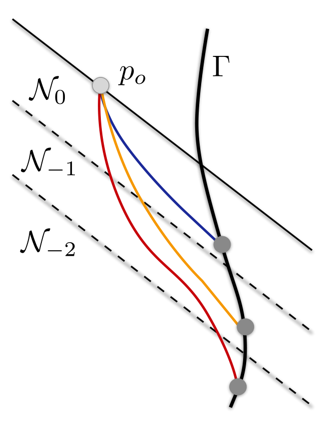
To fix the notation, let denote a fixed observation event and the timelike worldline of a point source. Assume that may be parametrized by an everywhere- function . The phase coordinate serves as a useful “quasi-time” [21] for plane wave spacetimes33 3 is not a “true” time function because is null. Generically, there do exist well-behaved functions where is everywhere timelike [41]. These are time functions in the usual sense, although they do not appear to simplify any computations performed here. Incidentally, the existence of such time functions implies that plane wave spacetimes are stably causal. Plane waves are not, however, globally hyperbolic [42]. Hypersurfaces of constant are not Cauchy surfaces., so let satisfy for all . The source’s worldline is not required to be geodesic.
This section establishes that under generic conditions, an ideal observer at may see exactly one image of from each of the “epochs” described in Sect. 2.2. Somewhat more precisely, there typically exists exactly one future-directed null geodesic from
| (40) |
to for each such that exists. See Fig. 2. Recall that the boundaries of depend only on the spacetime under consideration, and not at all on the behavior of any particular source. This allows generic bounds to be placed on time delays associated with the various images that may be observed.
Recall from Sect. 2.2 that each point in is connected to via exactly one (not necessarily null) geodesic. Synge’s function is therefore well-defined and explicitly given by (37) for all such that . Consider instead the rescaled function
| (41) |
If , the domain of is equal to all such that . If , we additionally suppose that for reasons of causality. Images of produced by a plane gravitational wave correspond to the zeros of .
Recalling the form (37) for , it is clear that depends on as well as the matrices , , , and . We have assumed in Sect. 2.1 that and are at least . So is . The definition of ensures that everywhere is defined. is therefore and is continuous.
is also monotonic. To see this, note that (9), (13), (14), (37), and (41) may be used to show that
| (42) |
is both continuous and monotonic, so at most one zero can exist for each . This means that at most one image of a source may reach an observer from each epoch . Exactly one such image exists if some are known to satisfy
| (43) |
Such bounds are easily established.
3.1 Lensing between conjugate hyperplanes
The simplest case to consider is one where lies “in between” hyperplanes conjugate to . Suppose that both and exist for some . This is true in Fig. 2 for . More generally, (38) and (39) imply that if there are no geodesics connecting to either or ,
| (44) |
It follows from these limits together with continuity that is surjective on . Since this function is also monotonic, there must exist exactly one emission phase such that and are connected by a null geodesic.
Under the same assumptions, projectiles moving on timelike geodesics may be thrown from to only if . Choosing to be sufficiently small (but positive), these projectiles can require an arbitrarily large amount of proper time to intersect . It is somewhat curious that points satisfying cannot be connected to by any causal geodesic. Such points may, however, be reached by suitably accelerated curves which are everywhere causal.
3.2 The youngest image
Next, consider the case when there exists at least one conjugate hyperplane in the observer’s past (as occurs in the example illustrated by Fig. 2). The arguments given above imply that if is geodesically disconnected from ,
| (45) |
The other boundary of the domain of occurs at . Here,
| (46) |
This limit clearly tends to if . Physically, implies that cannot be connected to by any null geodesic. Assuming that this is true, there must exist exactly one such that and are connected by a null geodesic.
3.3 The oldest image
The results of Sects. 3.1 and 3.2 typically suffice to describe the images formed in plane wave spacetimes containing an infinite number of conjugate hyperplanes in an observer’s past. It is, however, important to consider cases where only a finite number of conjugate points exist. This occurs, e.g., for finite wavepackets where has compact support. It is also true of linearly polarized vacuum waves that are tame in the sense described in [20].
If there is at least one conjugate hyperplane in the observer’s past, let denote the smallest negative integer such that exists. If there are no conjugate hyperplanes in the observer’s past, set . The case illustrated in Fig. 2 corresponds to if extends into the infinite past. Regardless, we ask whether there exist any future-directed light rays from to . Unlike in the cases considered above, sources spend an infinite amount of proper time in .
Even in flat spacetime, a source that accelerates for an infinitely long time may be causally-disconnected from certain observers via a Rindler horizon. Such phenomena can be ruled out here by supposing that there exists some finite constant such that
| (47) |
for all less than some cutoff. As is clear from (25) and (26), the left-hand side of this inequality acts like the square root of a time dilation factor between the coordinate and the source’s proper time. Eq. (47) implies that the source’s 4-velocity satisfies
| (48) |
sufficiently far in the past. It therefore excludes sources which experience arbitrarily large boosts against the background gravitational wave in the distant past. It is satisfied by, e.g., sources whose motion is geodesic sufficiently far into the past. Assuming that exists, it is clear from (42) that may be chosen sufficiently small that
| (49) |
Further assuming that is geodesically disconnected from (if ) or that is not null-separated from (if ), it follows that there exists exactly one smaller than (if ) or (if ) such that is connected to via a future-directed null geodesic.
3.4 Total image count for generic sources
The results just described may be summarized as follows: Suppose that there does not exist any past-directed geodesic segment from to whose endpoints are conjugate (in the usual sense). Also assume that the source and observer are not instantaneously aligned with the background wave: . If there exists an “oldest” phase conjugate to , further require that there be some such that the source’s motion is bounded by (48) sufficiently far in the past.
For each , these assumptions imply that an observer at sees exactly one image of as it appeared in . This provides a strong bound on the possible emission times of different images. If exists for every negative integer , an infinite number of images are formed. If, however, there is some smallest such that exists, images appear at . Note that these results depend only on the waveform and the phase coordinate associated with the observer. The total number of images is the same for all sources satisfying the hypotheses outlined above.
These hypotheses are generic. Recalling (21), the requirement that exclude any points conjugate to along a connecting geodesic is equivalent to demanding that the source’s worldline avoid certain well-behaved one- or two-dimensional subsets of the three-dimensional hyperplanes conjugate to . Similarly, the assumption that demands only that avoid a certain line on . The bound (48) on a source’s asymptotic 4-velocity can fail to hold only for sources which accelerate for an infinitely long time. Violating any of these conditions for a fixed observer would require that a source’s worldline be quite exceptional. Moreover, we now show that images appear under even broader (but more difficult to state) conditions than those just discussed.
3.5 Non-generic imaging
Despite the comments made above, our assumptions on the behavior of a source’s worldline can be violated in certain cases. Suppose, contrary to these assumptions, that there exists at least one point which is conjugate to along a geodesic connecting these two points. An infinite number of geodesics then pass between and . If the connecting geodesics are null, lies on a caustic of the observer’s past light cone. Continuous images of point sources – “Einstein rings” – are then formed at (ignoring the associated breakdown of geometric optics). Such cases are not considered any further here. If conjugate points between the source and observer are associated with non-null geodesics, discrete images of appear at . In these cases, the methods used above are easily adapted to find how many images of arrive at . As already mentioned, there can be no more than one root for each . Depending on the details of the system, the associated image from may or may not exist.
The case considered in Sect. 3.1 where lies in between successive conjugate hyperplanes is the simplest to analyze. Assuming that does not intersect the caustic of , no images are formed of if either is connected to via a timelike geodesic or is connected to via a spacelike geodesic. Otherwise, exactly one image exists from this region.
If there exists an oldest conjugate hyperplane as described in Sect. 3.3, suppose that the source satisfies (47) for some . There are then zero images of if is connected to via a timelike geodesic. There is exactly one image if these points are either geodesically disconnected or are connected by a spacelike geodesic.
The last cases to consider concern images of . First suppose that . If there exists at least one conjugate hyperplane in the observer’s past, one image is formed of if either is geodesically disconnected from or it is connected by a timelike geodesic. No images are formed if and are connected by a spacelike geodesic. If and there are no conjugate points in the observer’s past, condition (47) implies that there exists exactly one image of .
Cases where the source and observer are instantaneously aligned are more interesting. Suppose that . There then exists one image of with . Recalling that is not in the domain of , it is possible for a second image to be emitted from if somewhere. This may be seen by noting that
| (50) |
Two images of can therefore exist when and .
If a source includes points which are conjugate to the observer (in the ordinary sense), there is no simple result for the total number of images formed. Nevertheless, it is always possible to say that the total number of images is less than or equal to if a source does not intersect a caustic of the observer’s light cone.
4 Properties of lensed images
Plane wave spacetimes typically produce multiple images of each source. Even for sources whose intrinsic properties remain constant, these images can appear with different spectra, brightnesses, etc. We now compute these properties for generic configurations satisfying the hypotheses summarized in Sect. 3.4.
For each image of a timelike worldline seen at , there is an associated null geodesic segment connecting to an appropriate emission point . In terms of Synge’s function (36), these points satisfy
| (51) |
First derivatives of are always tangent to the connecting light ray. In particular, the vector
| (52) |
at points along the geodesic which eventually intersects (and is therefore past-directed). The derivative operator here is understood to act on the second argument of . Also note that is normalized such that . Parallel-transporting to the observation point yields
| (53) |
The derivative operator in this equation is understood to act on the first argument of . Both and may be viewed as (dimensionless) separation vectors between and .
Eq. (37) and the various identities of Sect. 2.1 may be used to compute the explicit coordinate components of and . Components transverse to the direction of wave propagation are
| (54) |
where and denote the transverse coordinates of the observer and source. A similar calculation shows that
| (55) |
and are related via
| (56) |
Much of the discussion below considers sources moving on geodesics. In these cases, use of (23) shows that
| (57) |
Here, . The various identities involving and discussed in Sect. 2.1 may also be used to reduce the imaging condition (51) to
| (58) |
Here, . Eq. (58) is a nonlinear relation for the emission “time” in terms of the observer’s position and the parameters , , , describing the source’s worldline. As discussed in Sect. 3, there can be many solutions to (58). These correspond to different images.
Neither nor depends on the observer’s motion. Nevertheless, redshifts and angles on the observer’s sky do depend on that motion (as is true even in flat spacetime). It is often useful to fix this effect by supposing that the observer is instantaneously comoving with the source. Following (32), this is taken to mean that the unit 4-velocities of the source and observer on satisfy
| (59) | |||
| (60) |
Recall from Sect. 2.3 that the “transverse momentum” is generated by contracting with the two Killing fields equal to at and having vanishing first derivative at that point. Also note that (60) implicitly defines an instantaneous observer velocity normalized (like ) such that .
4.1 Frequency shifts
Gravitational lenses typically discussed in astrophysics involve nearly-Newtonian mass distributions which may be regarded as approximately stationary (at least on sub-cosmological timescales). If both a source and an observer are sufficiently far from such a lens, there can be no significant redshift or blueshift from the gravitational field of that lens. Roughly speaking, a light ray falling into any stationary gravitational potential must climb out of that same potential. This result breaks down if light passes through non-stationary regions of spacetime. Indeed, plane wave spacetimes may produce images with significant frequency shifts [19].
Consider an approximately monochromatic beam of light emitted from and received at . A future-directed tangent vector to the emitted light ray may always be chosen such that
| (61) |
is the angular frequency of the light as seen by its source. The frequency of this same light ray as measured by an observer at is , where is equal to parallel transported from the source to the observer. The observed and emitted frequencies are therefore related by
| (62) |
Here, and . The 2-vectors and appearing here are determined by the source and observer positions via (37), (51), (54), and (55). The resulting frequency shift is valid for all emission points not contained in a caustic of .
Now suppose that a source moves on a geodesic and that the observer is instantaneously comoving with this geodesic in the sense of (59) and (60). Then doesn’t depend on which image is chosen. Eqs. (56), (57), and the symmetry of may be used to rewrite (62) as
| (63) |
The matrix in parentheses on the right hand side of this equation acts like a metric for the “separation” 2-vector . If both eigenvalues of are negative, the source is necessarily redshifted. Conversely, sources are always blueshifted when this matrix is positive definite. If has both positive and negative eigenvalues, the sign of the frequency difference depends on the direction of . For special configurations, there is no frequency shift at all.
4.2 Angles
Various images formed from a single source appear at different points on an observer’s sky. Like redshifts, the relative angles between images change depending on an observer’s 4-velocity . The angle between two images arriving at with tangents and is
| (64) |
Simplifying,
| (65) |
This expression is valid for arbitrary source and observer configurations. Specializing to geodesic sources and comoving observers,
| (66) |
Here, and . It is evident that angles are largely controlled by the difference between at the two emission times.
Another interesting angle to consider is the observed separation between a single image (emitted at ) and a generator of the background gravitational wave. For arbitrarily moving source and observer configurations,
| (67) |
For observers comoving with geodesic sources,
| (68) |
This may be used to rewrite the angle between two different images partially in terms of the angles and those images make with . Using (66),
| (69) |
Similarly, the frequency shift (63) of an individual image may be rewritten as
| (70) |
It is evident from this equation that images which appear highly blueshifted to comoving observers must satisfy .
4.3 Image distortion and magnification
Thus far, all sources here have been modelled as though they were confined to timelike worldlines. Real objects are not pointlike, however. They form extended worldtubes in spacetime. Images of such worldtubes form null geodesic congruences which converge on . These images can be significantly distorted by the curvature of spacetime. It is simplest to quantify such distortions by first fixing a particular null geodesic passing between some part of the source and . Precisely which geodesic is chosen is not important. serves only as an origin from which to discuss nearby light rays connecting to other points in the source. Once this origin has been fixed, the image of an extended source may be described entirely using deviation vectors on (at least for sufficiently small sources). See Fig. 3.

Deviation vectors (or Jacobi fields) satisfy the geodesic deviation (or Jacobi) equation along . Letting denote the past-directed null vector tangent to and obtained by parallel-transporting from , every deviation vector is a solution to
| (71) |
This equation is linear, so must depend linearly on initial data. In particular, all deviation vectors can be written as linear combinations of appropriate bitensors contracted into the initial data44 4 Capital letters are used in this subsection to denote abstract indices associated with the observation point . This is done to avoid confusion when writing down two-point tensors such as [see (72)]. and . All light rays observed at must necessarily intersect that point, so it suffices to set . The first derivative of a deviation vector at describes an angular deviation between one point of an image and the center associated with . We therefore consider deviation vectors with the form
| (72) |
is known as a Jacobi propagator. It satisfies the Jacobi equation
| (73) |
along together with the initial conditions
| (74) |
Note that is a bitensor. It maps vectors at into vectors at others points on . The transverse components of are
| (75) |
where is the matrix defined in Sect. 2.1. Other components of may be deduced from the eigenvector relations [23]
| (76) | |||
| (77) |
All parts of an image must arrive at an observer along null geodesics. Additionally, an observer with 4-velocity can only measure angles of vectors orthogonal to . It therefore suffices to restrict attention to deviation vectors satisfying
| (78) |
at . These constraints restrict all interesting initial data to a two dimensional space. The orthonormal vectors
| (79) |
form a basis for this space at . They satisfy
| (80) |
Parallel-transporting to another point on yields
| (81) |
which forms a Sachs basis [1] on . Initial data appearing in (72) must be of the form
| (82) |
where is an unconstrained 2-vector. The factor is included here so that is directly related to angles on an observer’s sky. A sufficiently small image may be described by a suitable set of 2-vectors representing the angular locations of each portion of the image with respect to the center defined by .
Each may be translated into a physical displacement at the source using (72) and (82). First note that for every particular , (76) implies that throughout . Indeed, is always a linear combination of the together with . Components of proportional to are physically irrelevant, so we consider only the Sachs components
| (83) |
Defining the matrix
| (84) |
it is then clear that for any . is referred to as the Jacobi matrix or Jacobi map [1, 11]. Using (75)-(77), (79), (81), and (84),
| (85) |
If a source moves on a geodesic which is instantaneously comoving with the observer,
| (86) |
This discussion implies that a portion of an image with angular separation from the fiducial direction associated with is spatially separated from the fiducial emission point by
| (87) |
The factors of have been introduced here to emphasize that this description is valid only for infinitesimal deviations. Regardless, (87) shows that up to the time dilation factor , the matrix central to all aspects of plane wave geometry may be physically interpreted as a transformation converting infinitesimal angles on the vertex of a light cone into infinitesimal separations elsewhere on that light cone. depends only on the coordinates of the source and emission points, and not on any other aspects of the physical configuration. It may be computed for all possible observer-source pairs directly from the wave profile .
Angles of emission (as opposed to observation) of the various light rays travelling from the source to the observer may be found by differentiating (87) and applying the appropriate time dilation factor:
| (88) |
The last equality here makes use of (62). Applying (87) shows that
| (89) |
The symmetric matrix therefore converts spatial locations to emission angles within the source (with the constraint that all light rays intersect ). It is referred to as the optical deformation matrix [1, 11].
Eq. (87) implies that there is a sense in which circles on the observer’s sky correspond to ellipses near . This deformation may be parametrized by performing a polar decomposition on :
| (90) |
Here, and represent rotation matrices through some angles and . The ratio is related to the ellipticity of the aforementioned ellipse. represents the angle between the principal axes of that ellipse and the Sachs basis. and are referred as shape parameters [1, 43].
Recalling that polarization vectors are parallel-transported in the geometric optics approximation [3], any polarization vector must have Sachs components which are constant along . In principle, the angle might therefore be measured by comparing the relative “rotation” between an object’s observed shape and an appropriate polarization angle [1, 44]. For linearly polarized waves where can be made diagonal by an appropriate coordinate choice, with respect to this coordinate system and the basis (81). It is shown in Sect. 6 that also vanishes in a natural way for all sufficiently weak wavepackets which are nonzero only for short times.
Eq. (87) implies that converts angles at the observer to separations within the source. The determinant of must therefore relate solid angles at to physical areas near :
| (91) |
It follows that
| (92) |
may be interpreted as an “angular diameter distance.” Absolute value signs are necessary here because changes sign after each pass through a conjugate hyperplane with multiplicity 1. Physically, such sign changes represent parity inversions of the resulting image. Note that does not necessarily increase monotonically with the age of an image (as computed using the source’s proper time).
Closely related to the angular diameter distance is the luminosity distance
| (93) |
One factor of arises here from considering light cones emanating from the source instead of the observer. The other factor of is related to the energy change associated with frequency shifts.
5 Symmetric plane waves
Now that various optical quantities have been computed for general plane wave spacetimes, we consider their application to various special cases. The simplest nontrivial plane waves are the symmetric waves. These are locally symmetric in the sense that . It follows from (3) that symmetric plane waves must have constant waveforms. Also note that is Killing in these examples [as well as , which is Killing in all plane wave spacetimes]. Particular symmetric plane waves may be specified entirely by the (constant) eigenvalues of .
Recalling the decomposition (6) of into , and , a coordinate rotation may always be used to set for symmetric waves. It is then evident that the two eigenvalues of are given by . It is always possible to set
| (94) |
where
| (95) |
The weak energy condition implies that , so at least one eigenvalue of must be negative (implying that at least one of the must be positive). We assume for definiteness that . Then,
| (96) |
If the vacuum Einstein equation is imposed, and . For conformally-flat geometries representing spacetimes associated with, e.g., pure electromagnetic plane waves, and . Other cases may be viewed as superpositions of gravitational and (“gravito”-)electromagnetic waves.
All symmetric waves produce an infinite number of images of almost every source. It is clear from (94) that these waves are also linearly polarized. The angles and appearing in (90) therefore vanish when considering image deformations with respect to the Sachs basis (81). Other lensing properties depend on the sign of . We call the case “gravity-dominated” and the case “matter-dominated.”
5.1 Gravity-dominated symmetric waves
Consider symmetric plane wave spacetimes where . Gravity-dominated waves such as these generalize the vacuum waves satisfying . Symmetric vacuum waves arise from, e.g., the Penrose limit of a null geodesic orbiting a Schwarzschild black hole on the light ring.
For any gravity-dominated symmetric wave, the matrices and defined in Sect. 2.1 are
It is clear that has an infinite number of zeros for any choice of . Each of these zeros represents a phase conjugate to . There are an infinite number of such phases in both the past and future of every observer. The discussion in Sect. 3 therefore implies that under generic conditions, an infinite number of images appear for almost every source. Explicitly, all conjugate phases are given by
| (103) |
where is any nonzero integer. It is evident from (19) that all of these phases have multiplicity 1. For any and any observation point with , exactly one image of each source is visible as that source appeared in . This corresponds to the region between and . Note that switches sign on each pass through a conjugate phase. The parity of an image emitted from is therefore opposite to the parity of an image emitted from .
Specializing to cases where the source is a geodesic and the observer is instantaneously comoving with that source on , some configurations lead to redshifts and others to blueshifts. Using (63),
| (104) |
An image is therefore redshifted if and only if
| (105) |
It is blueshifted when . There is no frequency shift at all in cases where
| (106) |
The direction of the frequency shift clearly depends only on the instantaneous orientation of the source and the observer on . In particular, it does not depend on which image is considered. All images of a particular source experience the same type of frequency shift.
Emission times for an observer comoving with a geodesic source may be found by solving (58). For gravity-dominated symmetric waves, this equation reduces to
| (107) | |||||
If , it is evident that the image from must satisfy . Images from the distant past are therefore emitted at phases very nearly conjugate to :
| (108) |
Substituting this relation into (68) and (104) shows that very old images cluster near on the observer’s sky and experience increasingly-negligible frequency shifts:
| (109) |
Old images of slightly extended sources are also highly distorted and demagnified. Their angular diameter and luminosity distances both scale like
| (110) |
Gravity-dominated symmetric waves therefore produce an infinite number of exponentially dimming images for almost every source.
5.2 Matter-dominated symmetric waves
Matter-dominated symmetric waves satisfying act somewhat differently than gravity-dominated waves. In these cases,
Phases conjugate to occur at and at , where are any nonzero integers. If is an irrational number, these two families of phases are distinct. Each conjugate pair then has multiplicity 1. If is rational, some conjugate pairs have multiplicity 2. In the conformally-flat case where , all conjugate phases have multiplicity 2. In every other case where is rational, an infinite number of conjugate phases occur with each multiplicity. Regardless of , an infinite number of images are formed for almost every source.
Now consider a luminous source moving on a geodesic. If the source and observer are instantaneously comoving in the sense of (59) and (60), frequency shifts associated with each image are given by (63). Since
| (117) |
is negative-definite in this case, all images are redshifted.
If , an image originating from must be emitted just before the source intersects . All such images cluster towards in the observer’s sky and have negligible frequency shifts. Images emitted near conjugate hyperplanes with multiplicity 1 are highly distorted. Images emitted near conjugate hyperplanes with multiplicity 2 are not significantly distorted at all. In both cases, however, older images are dimmer (although the rate at which this occurs is much slower than for gravity-dominated symmetric waves).
Regardless of the sign of , the oldest images formed by symmetric plane wave spacetimes depend on the spacetime structure at arbitrarily large transverse distances. If the metric is modified so that the wave decays at large distances, only a finite number of images discussed here would be unaffected. The oldest images found in pure symmetric waves likely do not appear at all in perturbed symmetric waves.
6 Sandwich waves
Symmetric plane waves are mathematically simple, but are not reasonable models for gravitational radiation emitted from compact sources. More interesting are waves where is nonzero only for a finite time: Sandwich waves. Suppose, in particular, that there exists some such that for all . It follows from (3) that such spacetimes are locally flat whenever or . The curved region containing the gravitational wave is effectively sandwiched between the two null hyperplanes and . Every timelike curve eventually passes entirely through such a wave.
Before an observer interacts with the wave, spacetime is flat and optics is trivial. The case where an observer has already passed through the wave is more interesting. In this case, and reduce to their flat space forms
| (118) |
when . The forms of and inside the wave depend on the details of , and will not be discussed here. If , however, there always exist four constant matrices , , and such that
| (119) |
Note that the dots on and do not refer to derivatives in this case. They are only used as a labelling device. It follows from (17) that is independent of . Moreover,
| (120) |
If there were no wave at all, and .
In general, and have a simple physical interpretation. If two geodesics are comoving and have a transverse separation when , it follows from (23) that the transverse separation between these geodesics is immediately before they interact with the wave at . Similarly, the relative transverse velocity of these geodesics is when .
Interpretations for and are somewhat less direct. Consider two geodesics which intersect at some time after the wave has passed, but which have a relative transverse velocity at . The difference in transverse velocities between these two geodesics is then when . Similarly, the difference in the transverse positions of these geodesics is at . It follows that controls shifts in position that are independent of the time at which the two geodesics cross each other.
In principle, , , , may all be found by solving (9) if is known. At first glance, this would appear to imply that numbers are required to describe observations through a sandwich wave. The actual number of required parameters is somewhat less than this. First note that the Wronskian identity (13) implies that is a symmetric matrix. It also implies that
| (121) |
Further simplifications arise by recalling from (14) that and are symmetric. It follows that
| (122) |
are symmetric as well. These expressions are completely general, and hold for any sandwich wave. They significantly constrain the number of independent parameters needed to specify and . Equivalently, they limit the number of parameters that must be extracted from .
It follows from the arguments of Sect. 3 that the number of images of a generic source observable in any plane wave spacetime is governed by the number of hypersurfaces conjugate to the hypersurface containing the observation event . Continuing to assume that , all phases conjugate to must be smaller than . It follows from (20) and (119) that conjugate phases occurring before the wave may be found by solving
| (123) |
for all . This equation is quadratic, so at most two solutions exist. An observer ahead of the wave may therefore see at most three images of a source as it appeared behind the wave. There may also be at most one image of a source as it appeared ahead of the wave. In principle, any number of images may arise from inside the wave [where (119) is not valid] if is sufficiently large.
Conjugate phases found by solving (123) clearly depend on the observation time . Less obviously, the number of conjugate phases can also depend on . For an observer moving on a timelike worldline (where increases monotonically), new conjugate phases – and therefore new images – sometimes appear at discrete times. These images correspond to observation times where (123) momentarily degenerates to a linear equation. New images can therefore arise when and
| (124) |
If , the two solutions to this equation are
| (125) |
Only solutions satisfying are physically relevant. When a conjugate phase of this type first appears, it satisfies
| (126) |
The associated image therefore provides a picture of the infinitely distant past. Furthermore, an infinite amount of the source’s history appears to the observer within a finite amount of proper time. This implies that new images are highly blueshifted.
No matter how long an observer waits, no conjugate phase can exceed . The emission time for an associated image might therefore be expected to tend towards a constant value as . This means that a very large amount of proper time at the observer corresponds to only a small amount of proper time at a source. Images which appear suddenly and are initially highly blueshifted become highly redshifted at late times.
It is unclear precisely what these types of images imply. To the extent that geometric optics remains valid, all observers passing through momentarily see almost the entire universe appear infinitely blueshifted as it was in the infinitely distant past. Furthermore, (70) implies that all of the universe is briefly compressed into a single point on each observer’s sky. Of course, such phenomena lie outside the domain of geometric optics. They may even lie outside of the realm of test fields propagating on a fixed background spacetime. Extreme focusing events like these might indicate instabilities inherent in the plane wave geometry itself. It should, however, be noted that all of the infinities just alluded to are likely to have finite cutoffs in “realistic” plane waves which decay at large transverse distances.
Weak wavepackets
One important class of sandwich waves are those that are very weak and last only for a short time. In these cases, , , , and may be expanded as integrals involving successively higher powers of . To lowest order in such a scheme, and are approximately unaffected by the wave while inside of it. Assuming that , the first corrections to this assumption are
| (127) | |||
| (128) |
This approximation is consistent with (13) [and therefore (121) as well]. In terms of the matrices appearing in (119), , , and
| (129) |
Note that Eqs. (127) and (128) should be applied with care if involves many oscillations of an approximately periodic function. In these cases, the integral of can be very nearly zero. Terms nonlinear in might then be significant.
Assuming that (127) and (128) are indeed adequate approximations for and , a coordinate rotation may always be used to diagonalize . There then exist two constants and such that
| (130) |
In this sense, all sufficiently short gravitational plane waves act as though they are linearly polarized [so in (90)]. In terms of the individual wavefunctions appearing in (6),
| (131) | |||||
| (132) |
The transverse coordinates have also been chosen such that
| (133) |
If a wave satisfies the vacuum Einstein equation, and . More generally, it follows from the weak energy condition that
| (134) |
Now assume that the integral of is non-negative, which entails only a minimal loss of generality. Then,
| (135) |
We say that a wave is gravity-dominated if and matter-dominated if . These definitions are closely analogous to those used to classify symmetric plane waves in Sect. 5. There, a wave was said to be gravity- or matter-dominated depending on the sign of the constant appearing in (94).
For weak gravity-dominated wavepackets, there can be at most one phase conjugate to an observer satisfying . If this exists, it evident from (128) that
| (136) |
is conjugate to with multiplicity 1. This equation is valid only if . A conjugate phase therefore exists only for observers satisfying
| (137) |
Note that is the unique physically-relevant solution to (124) in the gravity-dominated case.
Waves that are matter-dominated (so ) also admit the conjugate phase (136) when satisfies (137). In the conformally-flat case where , this is the only conjugate phase. Unlike in the gravity-dominated case, the multiplicity of is equal to 2 for conformally-flat waves. In all other matter-dominated cases, has multiplicity 1 and a second conjugate phase is admitted (also with multiplicity 1) for all observers satisfying
| (138) |
This occurs at
| (139) |
Note that (138) is a more stringent condition than (137). As implied by the notation, .
Consider a point source moving on a timelike worldline in a weak sandwich wave spacetime. Such a source appears differently when observed at different times. It is clear that when , exactly one image of is viewable under generic conditions. As time passes, the wave eventually passes through the observer. A second image then appears when . This image is always emitted before the first. If the wave involves a sufficient amount of Ricci curvature55 5 Distinguishing between different cases based on the Ricci tensor inside a wave requires that the approximations leading to (127) and (128) be valid. It is possible for, e.g., sufficiently strong vacuum waves to admit two conjugate phases in the region . (from e.g., electromagnetic plane waves) and is not conformally-flat, a third image appears when . This is emitted before the first two images. All images persist indefinitely once they appear. Sufficiently far in the future, one image is observed of the source as it appeared after interacting with the gravitational wave. All other images predate this interaction. See Fig. 4.
When the second image first appears at , the new conjugate phase is divergent. At all later times, it is finite. The same is also true for the emission times associated with the second image. Almost the entire past history of the source is therefore observable within a finite proper time. This implies an infinite blueshift. At late times, . The observed evolution of the source via the second image effectively freezes as asymptotes to (which predates the source’s interaction with the wave). Images such as these are highly redshifted, as indicated in Fig. 5. Note that a similar transition from infinite blueshift to infinite redshift also applies to the third image if it exists.
Another qualitative feature of the emission times plotted in Fig. 4 is that there is a sense in which pairs of images can “switch roles.” Consider, e.g., the left panel of that figure. At late times, the solid curve (corresponding to the younger image) is perfectly linear. Indeed, it remains very nearly linear until . A rapid transition then occurs where the dashed curve effectively takes over this linear behavior while the solid curve strongly deviates from it. In a sense, the two images reverse their roles. This phenomenon occurs one more time (somewhat less sharply) around when the second image first appears. It arises essentially because for the younger image and for the older image. These constraints can cause emission curves to bend sharply – with large accompanying frequency shifts – in order to avoid intersecting . Whether or not this occurs depends on whether the “average” linear increase of ever comes near . If it does, this role switching occurs. If not, the younger image is barely affected by the gravitational wave at all. This is illustrated in Fig. 6, where emission curves for several sources are plotted simultaneously.
To summarize, images which appear at discrete times briefly appear as bright, highly blueshifted “flashes.” Indeed, Fig. 7 shows that their luminosity distances go to zero. Simultaneously, the angular diameter distance of each new image tends to infinity. It is implied by (70) that all highly blueshifted images make must a very small angle with on the observer’s sky. The second (and third) images therefore appear aligned with the direction of propagation of the gravitational wave when they first appear. This direction could be quite different from the location of the other image(s). As time progresses, all images migrate across the observer’s sky as illustrated in Fig. 8. Different images may remain separated from each other by large angles at all times.
7 Discussion
Despite their simplicity, plane gravitational waves behave in qualitatively different ways from lenses associated with quasi-Newtonian mass distributions. As expected from their dynamic nature, plane waves generically shift the observed frequencies of various images. They may also admit images which appear to move, deform, change brightness, and shift color as time progresses.
More subtle differences relate to the number of images that are produced of a given source. For example, even numbers of images can appear generically (which has led plane wave spacetimes to be cited [1] as well-behaved examples where the odd number theorem [5, 7] does not apply). Some plane waves can even produce an infinite number of discrete images. Perhaps most striking of all are the bright flashes shown to be produced by generic sandwich waves in Sect. 6. These correspond to individual images which appear at discrete times. More typical gravitational lenses can produce new images if a source crosses an observer’s caustic. Individual images then split into two (or vice versa). The flashes produced by sandwich waves are quite different. Their appearance does not require that a source pass through an observer’s caustic. Such images appear individually from the infinitely distant past. Initially, they are infinitely bright and infinitely blueshifted points of light appearing in the direction of propagation associated with the gravitational wave.
Many of these effects depend at least partially on the idealization that a plane wave extends undiminished to infinitely-large transverse distances. Plane wave spacetimes are not asymptotically flat. Despite being topologically trivial and locally well-behaved, they are not even globally hyperbolic: Null geodesics passing between appropriately-chosen pairs of points can extend to arbitrarily large transverse distances in between those points. It is this property which permits the infinite number of images described in Sect. 5 to be produced by symmetric waves. The flashes described in Sect. 6 also depend on the spacetime structure at arbitrarily large distances. This structure likely affects the formation of even numbers of images as well. Indeed, the usual proofs of the odd number theorem require global hyperbolicity, among other assumptions [1, 5] (see, however, [7] for a more general formulation).
If a spacetime has the geometry of a plane wave only out to some finite transverse distance, all results derived here remain valid if the associated images involve light rays which never extend sufficiently far to interact with any large-distance modifications. The infinite sequence of images formed by a symmetric plane wave would then be expected to become finite for spacetimes which are only approximately plane waves. Calculations involving the oldest images could no longer be trusted in these cases. Similarly, the bright flashes associated with ideal sandwich waves are likely to be somewhat less extreme for waves which decay at infinity. Large brightnesses and large blueshifts can still exist, but these will be cut off at some finite maximum. Such maxima may, however, remain quite large.
It is reasonably clear that modifications of the geometry at large distances can remove some images. Less obviously, these modification can also introduce new images. Consider, for example, the -wave spacetimes obtained by substituting
| (140) |
in the metric (1). These generalize the plane wave spacetimes. It has been shown that if grows subquadratically as , the resulting geometries are globally hyperbolic [45]. Moreover, every pair of points is connected by at least one geodesic in these cases (unlike in pure plane wave spacetimes where the growth of is precisely quadratic). This implies that modifications of the geometry at large transverse distances can introduce new null geodesics even between points at small transverse distances. It would be interesting to explore these effects in more depth to understand precisely how modifications of this sort (or more general ones) alter the lensing properties described here for ideal plane waves. It would also be interesting to better understand what the transient flashes of Sect. 6 imply for waves propagating on plane (or almost-plane) wave spacetimes. This can likely be facilitated by the Green functions derived in [23].
References
References
- [1] Perlick V 2004 Living Rev. Relativity 7 9
- [2] Petters A O, Levine H and Wambsganss J 2001 Singularity theory and gravitational lensing (Boston, MA: Birkhäuser)
- [3] Schneider P, Ehlers J and Falco E E 1992 Gravitational Lenses (New York, NY: Springer-Verlag)
- [4] Petters A O and Werner M C 2010 Gen. Rel. Grav. 42 2011
- [5] McKenzie R H 1985 J. Math. Phys.26 1592
- [6] Perlick V 1996 Class. Quantum Grav.13 529
- [7] Perlick V 2001 Comm. Math. Phys. 220 403
- [8] Ehlers J and Newman E T 2000 J. Math. Phys.41 3344
- [9] Friedrich H and Stewart J M 1983 Proc. R. Soc.London A 385 345
- [10] Frittelli S and Newman E T 1999 Phys. Rev.D 59 124001
- [11] Seitz S, Schneider P and Ehlers J 1994 Class. Quantum Grav.11 2345
- [12] Werner M C 2009 J. Math. Phys.50 082504
- [13] Blandford R and Narayan R 1986 Astrophys. J. 310 568
- [14] Damour T and Esposito-Farèse G 1998 Phys. Rev.D 58 044003
- [15] Kovner I 1990 Astrophys. J. 351 114
- [16] Frieman J A, Harari D D and Surpi G C 1994 Phys. Rev.D 50 4895
- [17] Faraoni V 2008 New Astron. 13 178
- [18] Faraoni V 1998 Int. J. Mod. Phys. D 7 409
- [19] Faraoni V 1991 Gen. Rel. Grav. 23 583
- [20] Ehrlich P E and Emch G G 1991 The conjugacy index and simple astigmatic focusing Geometry and nonlinear partial differential equations eds V Oliker and A Treibergs (Providence, RI: American Mathematical Society)
- [21] Ehrlich P E and Emch G G 1993 Geodesic and causal behavior of gravitational plane waves: astigmatic conjugacy Differential Geometry: Geometry in mathematical physics and related topics eds R E Greene R E and S-T Yau (Providence, RI: American Mathematical Society)
- [22] Beem J, Ehrlich P and Easley K 1996 Global Lorentzian geometry (New York, NY: Dekker)
- [23] Harte A I and Drivas T D 2012 Phys. Rev.D 85 124039
- [24] Hollowood T J and Shore G M 2008 J. High Energy Phys. 12 091
- [25] Hollowood T J, Shore G M and Stanley R J 2009 J. High Energy Phys. 08 089
- [26] Bondi H and Pirani F A E 1989 Proc. R. Soc.London A 421 395
- [27] Bondi H, Pirani F A E and Robinson I 1959 Proc. R. Soc.London A 251 519
- [28] Penrose R 1976 Any spacetime has a plane wave as a limit Differential geometry and relativity eds. M Cahen and M Flato (Dordrecht: Reidel)
- [29] Blau M, Frank D and Weiss S 2006 Class. Quantum Grav.23 3993
- [30] Berenstein D, Maldacena J M and Nastase H 2002 J. High Energy Phys. 04 013
- [31] Grignani G, Harmark T, Marini A and Orselli M 2010 J. High Energy Phys. 06 034
- [32] Stanley R and Hollowood T J 2011 J. High Energy Phys. 10 096
- [33] Wald R M 1984 General relativity (Chicago, IL: University of Chicago Press)
- [34] Eardley D M, Lee D L and Lightman A P 1973 Phys. Rev.D 8 3308
- [35] Pravda V, Pravdovà A, Coley A and Milson R 2002 Class. Quantum Grav.19 6213
- [36] Torre C G 2006 Gen. Rel. Grav. 38 653
- [37] Günther P 1988 Huygens’ principle and hyperbolic equations (London: Academic Press)
- [38] Etherington I M H 1933 Phil. Mag. 15 761
- [39] Ellis G F R 1971 Relativistic cosmology General relativity and cosmology: Proceedings of the 47th international school of physics “Enrico Fermi” ed R K Sachs (New York, NY: Academic Press)
- [40] Hartman P 1982 Ordinary Differential Equations (Boston, MA: Birkhäuser)
- [41] Hubeny V, Rangamani M and Ross S 2004 Phys. Rev.D 69 024007
- [42] Penrose R 1965 Rev. Mod. Phys.37 215
- [43] Frittelli S, Kling T P and Newman E T 2000 Phys. Rev.D 63 023006
- [44] Surpi G C and Harari D D 1999 Astrophys. J. 515 455
- [45] Flores J L and Sánchez M 2006 Lect. Notes Phys. 692 79