-titleUHECR2012 Symposium
Nitrogen fluorescence in air for observing extensive air showers
Abstract
Extensive air showers initiate the fluorescence emissions from nitrogen
molecules in air. The UV-light is emitted isotropically and can be used
for observing the longitudinal development of extensive air showers in the
atmosphere over tenth of kilometers. This measurement technique is well-established
since it is exploited for many decades by several cosmic ray experiments.
However, a fundamental aspect of the air shower analyses is the description
of the fluorescence emission in dependence on varying atmospheric conditions.
Different fluorescence yields affect directly the energy scaling of air shower
reconstruction. In order to explore the various details of the nitrogen
fluorescence emission in air, a few experimental groups have been performing
dedicated measurements over the last decade. Most of the measurements
are now finished. These experimental groups have been discussing their
techniques and results in a series of Air Fluorescence Workshops
commenced in 2002.
At the 8th Air Fluorescence Workshop 2011, it was suggested to
develop a common way of describing the nitrogen fluorescence for application
to air shower observations. Here, first analyses for a common treatment of
the major dependences of the emission procedure are presented. Aspects like
the contributions at different wavelengths, the dependence on pressure as
it is decreasing with increasing altitude in the atmosphere, the temperature
dependence, in particular that of the collisional cross sections between
molecules involved, and the collisional de-excitation by water vapor are discussed.
1 Introduction
The detection of ultra-high energy cosmic rays is very challenging and it is a major key to answer open questions in astroparticle physics. Cosmic rays are messengers of processes in their sources and at their propagation towards us. Two important aspects of the cosmic ray properties are their energy and mass composition in order to evaluate the shape of the cosmic ray spectrum [1].
For detecting ultra-high energy cosmic rays, extensive air showers initiated in the Earth’s atmosphere are observed. Manifold techniques have been developed over the last decades and in this article, we will focus on the fluorescence technique.
While extensive air showers are developing through the atmosphere, their energy deposit causes an excitation of atmospheric nitrogen molecules. The spontaneous de-excitation can be separated into a radiative and a non-radiative channel. The isotropically emitted UV fluorescence light is proportional to the energy deposit and can be used to perform an almost calorimetric measurement of the air shower energy [2]. The fluorescence technique was investigated initially in [3] and found its successful application at Fly’s Eye [4], HiRes (High Resolution Fly’s Eye experiment) [5], the Pierre Auger Observatory [6], and TA (Telescope Array) [7]. With JEM-EUSO (Extreme Universe Space Observatory onboard the Japanese Experiment Module), there are even plans to put this fluorescence technique onboard the ISS11 1 International Space Station to observe extremely high-energy cosmic rays from space [8].
For determining the absolute fluorescence yield, its emission spectrum, as well as its dependence on varying atmospheric conditions to an appropriate level of precision, several experimental groups have been performing dedicated laboratory measurements over the last decade. The experimental efforts have been supplemented by several simulations and air shower reconstruction studies. These groups have been discussing their techniques and data in a series of Air Fluorescence Workshops (AFW) commenced in Utah, 2002 [9]. Main results are contributed by the following alphabetic list of collaborations and groups led by their principal investigators: AIRFLY [10, 11, 12, 13, 14, 15], Airlight [16, 17], Arqueros/UCM [18, 19, 20, 21, 22], FLASH [23, 24, 25, 26], Fraga/LIP [27, 28], Keilhauer/KIT [29, 30, 31], Lefeuvre/APC [32], MACFLY [33], Nagano/Sakaki [34, 35, 36], and Ulrich/TUM [37, 38, 39, 40]. At the up to now last Air Fluorescence Workshop in Karlsruhe, 2011, it was decided to develop a common fluorescence description for application at air shower reconstructions [9]. The description of the fluorescence emission can be summarized by three different aspects – the absolute fluorescence yield, e.g. at a representative band head, the wavelength-dependent spectrum, and the dependence on atmospheric conditions. At a first step, the two dependences are being discussed to be able to compare reconstructions of extensive air showers based on a common altitude-dependent shape of the fluorescence emission. In a second step, the challenge of determining the absolute fluorescence yield is being addressed which directly introduces the scaling of the reconstructed primary energy of air showers.
2 Description of the fluorescence emission from molecular nitrogen in air
The fluorescence light initiated by extensive air showers is mainly produced by the energy deposit of electrons/positrons from the air shower in inelastic collisions with air molecules. The observed emission is dominated by radiative de-excitation of N2 and N in the wavelength range between about 290 and 430 nm. The radiative de-excitation is competing with quenching processes caused by further non-excited molecules in air. Thus, the fluorescence yield , given as the number of photons emitted per unit deposited energy, can be determined by the intrinsic fluorescence yield at zero pressure reduced by the non-radiative de-excitation. Here, we follow the nomenclature as defined in [2]. The de-excitation processes can either be described by the natural lifetime of an excited state together with the quenching rate constant or collisional cross sections (cf. [3], [16, 17], [37, 38, 39, 40]) or by introducing a reference pressure , at which the probability of collisional quenching equals that of radiative de-excitation, in the Stern-Volmer factor [41].
In this monograph, we employ the formulation using the Stern-Volmer factor for the fluorescence yield as a function of the photon wavelength and atmospheric conditions
| (1) |
and taking into account the temperature-dependent collisional cross sections between excited nitrogen and air molecules in general by
| (2) |
The reference atmospheric condition at which the laboratory fluorescence measurements have been carried out is denoted by . The wavelength dependence of the fluorescence intensity is expressed as which is relative to that wavelength at which the absolute yield is determined. The leading factor of the right side of Eq. (1), , gives the absolute yield at nm where the emission from N2 is strongest in the observation range. In Eq. (2), is the exponent of the power law describing the temperature-dependent collisional cross sections for each wavelength.
For humid air, the characteristic pressure for dry air has to be substituted in the denominator of Eq. (1) by
| (3) |
where is the characteristic pressure for collisional quenching with water vapor and is the partial pressure of water vapor in the atmosphere.
Above, the different factors are written in dependence on . However, the spectral emissions are mainly vibrational transitions from the Second Positive (2P) system of N2 and First Negative (1N) of N with some minor contributions from the Gaydon-Herman (GH) system of N2. Since the rotational structure of the molecular bands is not resolved in our experiments, the transitions can be described by molecular bands22 2 as vibrational quantum numbers of the upper and lower states with a spectral width and shape determined by the rotational structure. Concerning the spectral intensity of the emissions , each transition between corresponds to one wavelength and has, of course, its individual strength. For the factors describing the quenching effects, however, only the physical properties of the upper, excited state are of relevance. Thus, the characteristic pressures and as well as the exponent are the same for all transitions arising from the same upper vibrational level .
3 First draft of a common reference yield
As a first step, we describe the spectral and atmospheric dependences of the fluorescence emissions, see Sec. 1. This provides us a common altitude-dependent shape of the fluorescence profile. For application to air shower reconstructions, this requires an adequate knowledge of atmospheric conditions at the place and time of an observed air shower event [31].
The values for all necessary parameters to describe the fluorescence emission in air with the suggested procedure are summarized in Tab. 1 and will be discussed in more details in the following.
| system | band | |||||
|---|---|---|---|---|---|---|
| (nm) | (%) | (hPa) | (hPa) | |||
| N2 2P | 0-0 | 337.1 | 100 | 15.83 0.80 | 1.46 0.05 | -0.35 0.08 |
| 0-1 | 357.7 | 67.4 2.4 | ||||
| 0-2 | 380.5 | 27.2 1.0 | ||||
| 0-3 | 405.0 | 8.07 0.29 | ||||
| 1-0 | 315.9 | 39.3 1.4 | 12.03 0.66 | 1.90 0.18 | -0.20 0.08 | |
| 1-1 | 333.9 | 4.02 0.18 | ||||
| 1-2 | 353.7 | 21.35 0.76 | ||||
| 1-3 | 375.6 | 17.87 0.63 | ||||
| 1-4 | 399.8 | 8.38 0.29 | ||||
| 1-5 | 427.0 | 7.08 0.28 | ||||
| 2-0 | 297.7 | 2.77 0.13 | 13.12 0.71 | 1.80 0.14 | -0.17 0.08 | |
| 2-1 | 313.6 | 11.05 0.41 | ||||
| 2-2 | 330.9 | 2.15 0.12 | ||||
| 2-3 | 350.0 | 2.79 0.11 | ||||
| 2-4 | 371.1 | 4.97 0.22 | ||||
| 2-5 | 394.3 | 3.36 0.15 | ||||
| 2-6 | 420.0 | 1.75 0.10 | ||||
| 3-1 | 296.2 | 5.16 0.29 | 19.88 0.86 | 1.84 0.2 | -0.19 0.08 | |
| 3-2 | 311.7 | 7.24 0.27 | ||||
| 3-3 | 328.5 | 3.80 0.14 | ||||
| 3-5 | 367.2 | 0.54 0.04 | ||||
| 3-7 | 414.1 | 0.49 0.07 | ||||
| 4-4 | 326.8 | 0.80 0.08 | 19 5.0 | 1.84 0.2 | -0.19 0.08 | |
| 4-7 | 385.8 | 0.50 0.08 | ||||
| N 1N | 0-0 | 391.4 | 28.0 1.0 | 2.94 0.33 | 0.47 0.02 | -0.76 0.08 |
| 0-1 | 427.8 | 4.94 0.19 | ||||
| 1-1 | 388.5 | 0.83 0.04 | 3.92 0.32 | 0 | 0 | |
| 1-2 | 423.6 | 1.04 0.11 | ||||
| N2 GH | 0-4 | 346.3 | 1.74 0.11 | 7.98 0.56 | 0 | 0 |
| 0-5 | 366.1 | 1.13 0.08 | ||||
| 0-6 | 387.7 | 1.17 0.06 | ||||
| 5-2 | 308.0 | 1.44 0.10 | 21 10.0 | 0 | 0 | |
| 6-2 | 302.0 | 0.41 0.06 | 21 10.0 | 0 | 0 | |
| 6-3 | 317.6 | 0.46 0.06 |
3.1 Spectral intensities
For the values of , there is a quite complete and precise measurement from AIRFLY [10, 11]. The spectral resolution of these data is very high which enables an adequate consideration of all dependences. The data, which are adopted for the first suggestion of a common reference yield, are displayed in Fig. 1, along with data from further working groups. A similar set, in terms of resolution and accuracy, of wavelength- dependent intensities is obtained by [40]. However for the sake of consistency, the data set measured by AIRFLY was chosen for this fluorescence description.

3.2 Atmospheric dependences
The AIRFLY collaboration has published a complete set of () values in dry air, one for each band [10, 11]. As stated above, it is expected that all individual transitions starting at the same upper vibrational level have the same . Therefore, the suggestion is to use weighted averages of the values measured for bands of a particular molecular system with the same starting vibrational level. As weight factors, the quoted uncertainties are used. Because of the experimental technique, AIRFLY was running, for all transitions apart from the 337.1 nm line, there is not only a given uncertainty of the measurement itself, , but an additional value for the propagated uncertainty of the measurement of the 337.1 nm line, . To take into account both uncertainties, a minimization of with
| (4) |
is performed. The first term corresponds to the main transition N2 2P(0,0) at 337.1 nm, the second term to all other transitions of the 2P(0,) progression, and the double sum accounts for all other bands. The searched values for the different bands are denoted as in Eq. (4) and listed in Tab. 1 in the fifth column. The corresponding uncertainties are derived by maximizing the influence of to the remaining data by setting in the second and third term of Eq. (4). For the band progressions 2P(4,), GH(5,), and GH(6,), we follow the recommendation of AIRFLY [10].
The quenching by water vapor molecules in the atmosphere can be taken into account by applying Eq. (3) to Eq. (1). The additional reference pressure is determined experimentally at a given temperature . The group of Nagano/Sakaki has performed systematic studies about the effect of quenching excited nitrogen molecules by water vapor (cf. overview talk by N. Sakaki at the 8th AFW 2011 [43]). They measured for several wavelengths in two different ways. First, they analyzed the measurements of the photon yield and in a second step, they derived from lifetime measurements. The results are recalled in Tab. 2. As also discussed by A. Ulrich (cf. overview talk at the 8th AFW 2011 [44]), a systematic discrepancy was found between these two procedures. Even though the details are not fully understood yet, the overall uncertainties propagating into air shower reconstructions are sufficiently small.
| from photon yield | from lifetime | ||||
|---|---|---|---|---|---|
| Band | |||||
| (nm) | (hPa) | (hPa) | (hPa) | (hPa) | |
| 2P(0,0) | 337.1 | 1.36 | 0.07 | 1.68 | 0.13 |
| 2P(0,1) | 357.7 | 1.23 | 0.12 | 1.83 | 0.18 |
| 2P(0,2) | 380.5 | 2.08 | 0.34 | 2.01 | 0.27 |
| 2P(1,0) | 315.9 | 2.23 | 0.54 | 2.38 | 0.35 |
| 2P(1,4) | 399.8 | 1.30 | 0.29 | 2.26 | 0.41 |
| 2P(2,2) | 330.9 | 1.95 | 0.49 | 2.88 | 0.39 |
| 2P(2,4) | 371.1 | 1.62 | 0.28 | 1.59 | 0.2 |
| 1N(0,0) | 391.4 | 0.40 | 0.04 | 0.42 | 0.03 |
| 1N(0,1) | 427.8 | 0.53 | 0.07 | 0.89 | 0.07 |
Here, we suggest to average the weighted averages of the two independent data sets, again by applying the uncertainties as weights. The procedure and the propagation of the uncertainties is performed by
| (5) |
and
| (6) |
respectively. The final values are listed in Tab. 1. As indicated in Tab. 2, no data are given for several weaker transitions. In this case, we suggest to apply a weighted average of the values of and 2 for those of and 4. The emissions for the two weaker bands 2P(3,) and 2P(4,) contribute with 4.8% to the entire emission at atmospheric ground conditions (c.f. Tab. 1). For all other band systems, the is set to zero because of missing information but these transitions contribute with only 2.1% to the total intensity (c.f. Tab. 1).
A set of measurements of the -coefficient describing the temperature dependence of the quenching cross sections of the main bands of the 2P and 1N band systems in air is also provided by the AIRFLY Collaboration [13]. The most recent data have been presented at the 6th Air Fluorescence Workshop in L’Aquila, Italy [46]. Because of the same experimental technique, the -values are derived by following the same procedure as for . In the absence of further experimental data for weaker transitions, the weighted averages of values of and 4 are calculated correspondingly to the procedure for .
Having derived all necessary information to determine the fluorescence emission in air, an academic fluorescence yield profile is plotted in Fig. 2 for an 0.85 MeV electron. In addition, the fluorescence emission is plotted for the case of no water vapor quenching nor applying the temperature-dependent collisional cross sections (red, dashed line).

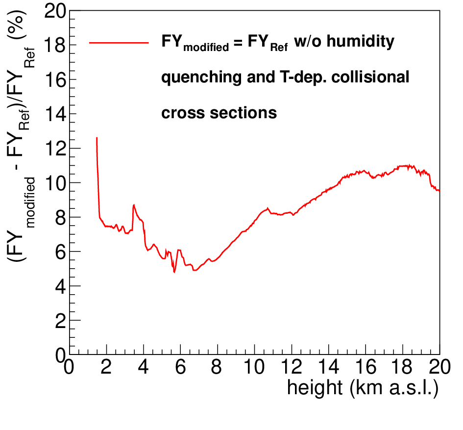
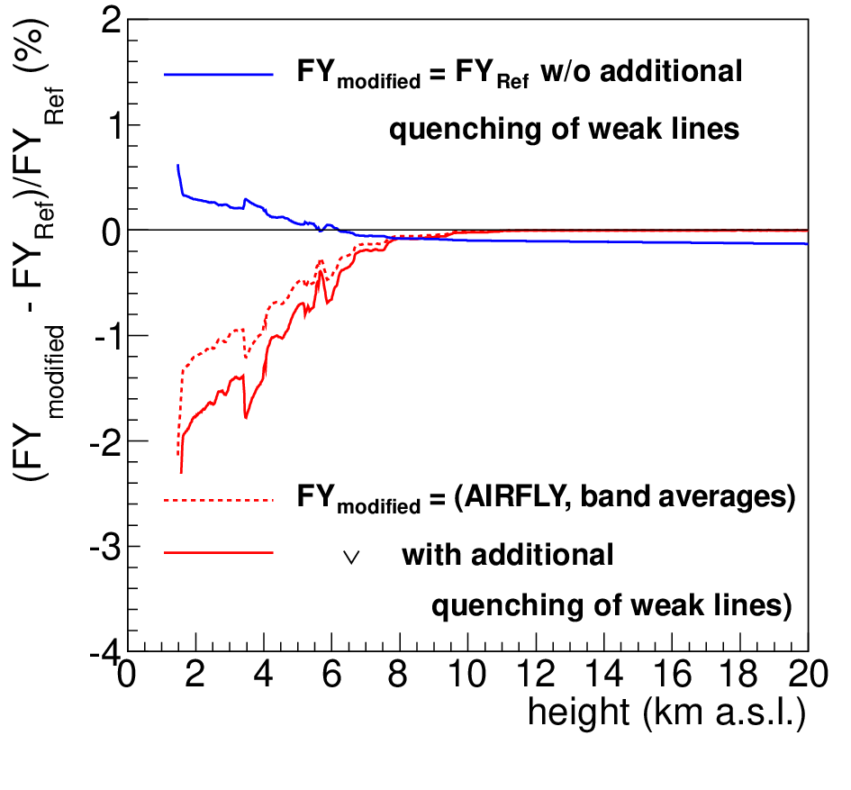
Some systematics about the choice of the suggested parameters for the reference description of the fluorescence emission are investigated and displayed in Fig. 3. For both, the quenching by water vapor and the temperature-dependent collisional cross sections, the effect of applying estimated values to the weaker transitions are presented.For the water vapor quenching, also another data set is shown for comparison (Fig. 3, left, red curves).
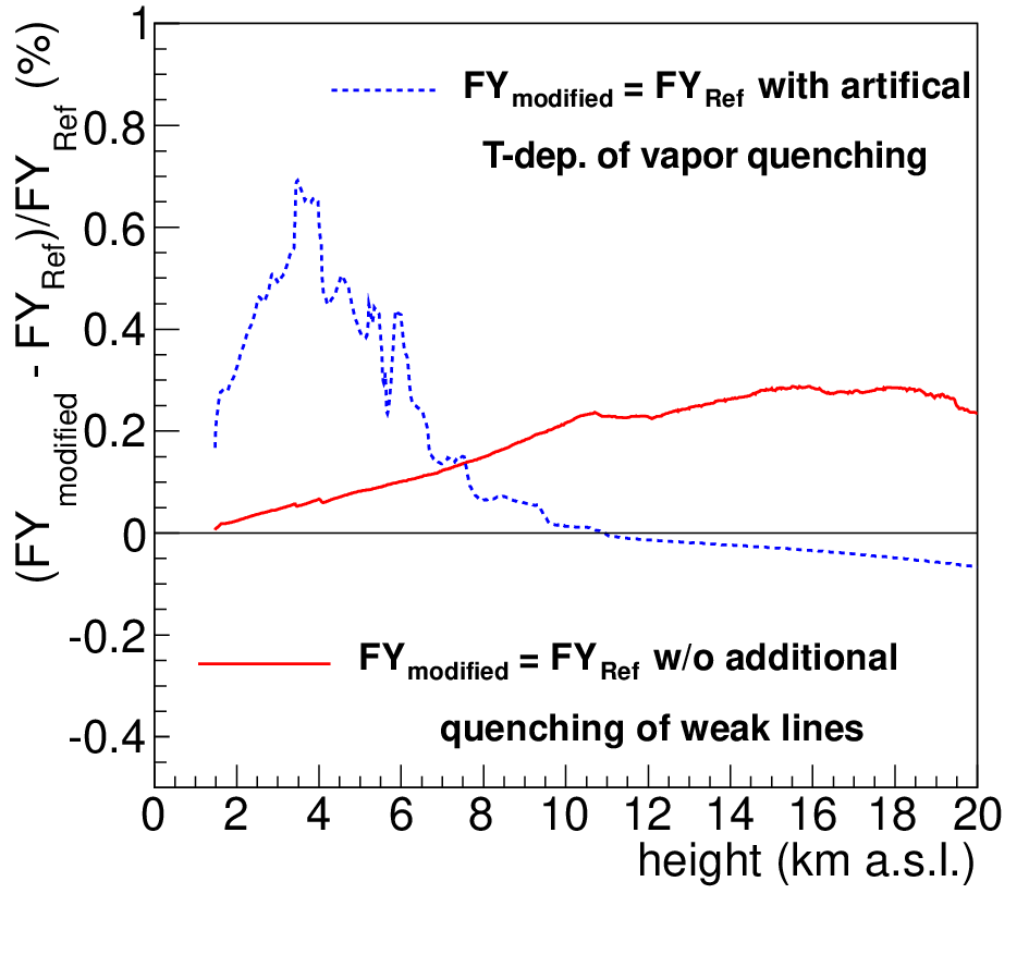
In the case of temperature-dependent collisional cross sections, there have been no measurements up to now to determine if there is also a temperature-dependence for the de-excitation by water vapor molecules. Thus, we applied an artificial dependence which is calculated with a factor of -5 to the known -values for water vapor to simulate a quite extreme case. As can be seen in Fig. 3, right, blue dotted curve, the overall variations are of minor importance.
4 Application to Air Shower Reconstruction
In the following, the reference description of the fluorescence emission is applied to full air shower reconstructions. Here, we use an exemplary set of high-quality hybrid events which have been observed during one year by the Pierre Auger Observatory with both detector components, the fluorescence detector and the surface detector for secondary particles [47, 48, 49]. The reconstructions are performed with the software framework [50] taking into account all necessary calibrations of the different detectors as well as actual atmospheric conditions in terms of profiles of atmospheric state variables and measured aerosol conditions [51, 52, 53]. The same set of air shower events is reconstructed in the same manner several times, only the description of the fluorescence emission is varied. To study how the fluorescence description affects the reconstruction results, we focus here on the air shower observables primary energy and position of shower maximum .
4.1 Reconstruction results with the same absolute scaling
For this reconstruction study, we use in all calculations the same absolute scaling of the fluorescence yield which is taken from Nagano et al. [35]. The fluorescence emission at 800 hPa and 293 K of the 337.1 nm line is 6.38 /MeV. The reconstruction set based on the reference fluorescence description S is taken as the ’standard’ and uses the data given in Tab. 1. The reconstruction set of the same data which uses the standard procedure of the Auger Observatory is labeled with SAuger_NaganoScale. Furthermore, the fluorescence description used in the TA experiment is implemented into the reconstruction of these air shower events obtained by the Auger Observatory and also scaled by the same fluorescence yield of the 337.1 nm line, STA_NaganoScale. In Fig. 4, the different sets of reconstructions are compared to that with the reference fluorescence description. On the left, the difference of the reconstructed primary energy of the air showers is given and on the right, the difference of the reconstructed position of shower maximum is shown. It should be mentioned that in the case of the TA-reconstruction, no temperature-dependent collisional cross sections and no humidity quenching is taken into account. The intensity spectrum is taken from the FLASH experiment, as shown in Fig. 1.


Right: Difference of reconstructed position of shower maximum of air showers. SAuger_NaganoScale- S: Mean 0.71 , RMS 1.25 ; STA_NaganoScale- S: Mean 1.63 ; RMS 3.56 .
In the following, some possible systematics are investigated. The fluorescence emission dominates the energy scale of the reconstructions, so the differences of the reconstruction sets are plotted vs. in the upper part of Fig. 5. While the dependence on is very flat and small for SAuger_NaganoScale both for the energy and reconstruction, a considerable dependence is found for STA_NaganoScale in particular for the reconstructed energy.


.


The atmospheric dependences are studied by analyzing the reconstructions vs. vertical of the air shower (Fig. 5, middle row) and vs. month (Fig. 5, bottom row). In the first case, the influence of different atmospheric profiles of the state variables on e.g. deeply or shallowly penetrating air showers are emphasized. There is hardly any systematics for the reconstructed energy, but the reconstruction of is affected. Because of the missing temperature-dependent collisional cross sections, very shallow air showers are reconstructed with a 4 larger for STA_NaganoScale than for S. The influence of the quenching by water vapor is emphasized for deeply penetrating air showers and small modifications of the reconstructed are found for both comparisons. The seasonal dependence is displayed on a monthly basis. Also here, no significant effects are visible for the reconstructed energy. For the reconstruction set STA_NaganoScale, a noticeable modulation with seasons can be seen for the reconstructed position of shower maximum.
Even though some modifications of the fluorescence emission are recognizable for the case of ignoring the additional temperature and humidity dependences (cf. Fig. 3), the overall effect to full air shower reconstructions is negligible. Only very few events have differences in the reconstructed primary energy, left part of Fig. 6, where the mean of the distribution is at -0.08% with an RMS of 0.7%. A similar picture is given for the reconstructed , right part of Fig. 6, where the mean of the distribution is at -0.003 with an RMS of 1.02 .


4.2 Discussion of different absolute scalings
In this part of the reconstruction study, different absolute scalings of the fluorescence yield are used. Typically, the absolute yield is determined for the main emission line at 337.1 nm and the spectral intensities of all other transitions are measured relatively to that main emission. For the reference description presented here, S, the absolute yield from Nagano et al. [35] is applied, together with the spectral intensities of AIRFLY [10]. Recently, the AIRFLY Collaboration has presented an own absolute yield for the 337.1 nm line, which is 7.07 /MeV at 800 hPa and 293 K, corresponding to 5.60(1) /MeV at 1013 hPa and 293 K [15, 54]. In the following, reconstructions using this absolute yield together with the reference description are labeled with S. The TA experiment typically applies in its reconstructions an intensity spectrum provided by the FLASH experiment for the entire wavelengths range between 300 and 420 nm together with an absolute scale from Kakimoto et al. for the total emission between 300 and 400 nm [55]. Converting this into an absolute yield of the main emission corresponds to 5.40 /MeV at 800 hPa and 293 K. The reconstruction set with these data is indicated by STA-FLASHScale. Very recently, the group of Ulrich et al. at the Technische Universität München - TUM also provided an absolute yield of the 337.1 nm line [40]. They derived a value of 6.3 /MeV at 1000 hPa and 293 K, which corresponds to 8.3 /MeV at 800 hPa and 293 K. The reconstruction set with this absolute yield, the spectral intensities also from TUM (cf. Fig. 1), and all other parameters as given for the reference yield is labeled with S. Finally, these values can be compared with a theoretical calculation performed by J. Rosado and F. Arqueros. With a sophisticated Monte Carlo simulation, they derive a value of 6.3 /MeV at 1013 hPa and 293 K [56, 57].
Applying the different absolute scales to the same air shower reconstruction as presented in Sec. 4.1, the differences for the reconstructed energy and can be analyzed, see Fig. 7.


The mean energy of S is shifted by -9.0% as compared with the reconstruction of the Auger Observatory SAuger_NaganoScale with an RMS of 1.5% (solid black line of Fig. 7, left). For , the mean is shifted by 1.1 (RMS 1.4 ) (solid black line of Fig. 7, right). Applying the scale derived from the TUM working group, the modification is even more extreme (dashed red line in Fig. 7). The mean reconstructed energy is shifted by -19.3% (RMS 2.4%) and the mean position of shower maximum by 3.0 (RMS 2.2 ). Comparing the reconstruction applying the fluorescence description of the TA experiment with that of the Auger Observatory gives a mean energy shift of 3.6% (RMS 1.8%). The mean is shifted by -2.0 with a large tail represented by an RMS of 4.1 .
5 Conclusions and Outlook
We presented a first suggestion of a common reference description of the fluorescence emission in air which is widely used for high-energy cosmic ray observations. For the spectral and atmospheric dependences, detailed parameters could be derived from different experimental studies. Smaller variations of these data are still possible because of some pending publication of experimental data and some improvements in our algorithms. However, the overall description of the altitude-dependent fluorescence emission has reached an appropriate level for air shower reconstructions. The absolute scaling is still to debate but we hope to revive the discussion with all parties to find a reasonable decision soon.
Acknowledgments
First of all, we want to thank the organizers of the inspiring UHECR2012 symposium. Furthermore, we thank all participants of the 8th Air Fluorescence Workshop, who gave us the mandate to develop a common reference description of the fluorescence emission. In particular, we acknowledge all colleagues of the ’fluorescence community’ who provided us their data and details about their experiments and helped us with fruitful discussion. And we are grateful to all (our) cosmic ray collaborations applying the fluorescence technique but especially the Telescope Array Collaboration and the Pierre Auger Collaboration for allowing us to use real event data and the reconstruction framework . Part of this work was funded by the Bundesministerium für Bildung und Forschung (BMBF) and by the Deutsche Forschungsgemeinschaft (DFG), Germany.
References
- (1) V. Berezinsky, these proceedings (2012)
- (2) F. Arqueros et al., Nucl. Instrum. Meth. A597 (2008) 1
- (3) A.N. Bunner, Cosmic ray detection by atmospheric fluorescence, Ph.D. Thesis, Cornell University (1967)
- (4) R.M. Baltrusaitis et al. (Fly’s Eye Collab.), Nucl. Instrum. Meth. A240 (1985) 410
- (5) T. Abu-Zayyad et al. (HiRes Collab.), Nucl. Instrum. Meth. A450 (2000) 253
- (6) J. Abraham et al. (Pierre Auger Collab.), Nucl. Instrum. Meth. A620 (2010) 227
- (7) H. Kawai et al. (TA Collab.), Nucl. Phys. B - Proc. Sup. 175-176 (2008) 221
- (8) A. Santangelo for the JEM-EUSO Collaboration, these proceedings (2012)
- (9) http://www.kceta.kit.edu/8afw2011
- (10) M. Ave et al. (AIRFLY Collab.), Astropart. Phys. 28 (2007), 41
- (11) M. Ave et al. (AIRFLY Collab.), Nucl. Instrum. Meth. A597 (2008) 41
- (12) M. Ave et al. (AIRFLY Collab.), Nucl. Instrum. Meth. A597 (2008) 46
- (13) M. Ave et al. (AIRFLY Collab.), Nucl. Instrum. Meth. A597 (2008) 50
- (14) M. Ave et al. (AIRFLY Collab.), Nucl. Instrum. Meth. A597 (2008) 55
- (15) M. Ave et al. (AIRFLY Collab.), Nucl. Phys. B - Proc. Sup. 212-213 (2011) 356
- (16) T. Waldenmaier et al., Astropart. Phys. 29 (2008) 205
- (17) T. Waldenmaier et al., Nucl. Instrum. Meth. A597 (2008) 67
- (18) F. Rosado et al., Nucl. Instrum. Meth. A597 (2008) 83
- (19) F. Arqueros et al., Nucl. Instrum. Meth. A597 (2008) 94
- (20) F. Arqueros et al., New J. Phys. 11 (2009) 065011
- (21) J. Rosado et al., Astropart. Phys. 34 (2010) 164
- (22) M. Monasor et al., Astropart. Phys. 34 (2011) 467
- (23) J.W. Belz et al. (FLASH Collab.), Astropart. Phys. 25 (2006) 129
- (24) R. Abbasi et al., Astropart. Phys. 29 (2008) 77
- (25) R. Abbasi et al. (FLASH Collab.), Nucl. Instrum. Meth. A597 (2008) 32
- (26) R. Abbasi et al. (FLASH Collab.), Nucl. Instrum. Meth. A597 (2008) 37
- (27) M. Fraga et al., Nucl. Instrum. Meth. A597 (2008) 75
- (28) L. Pereira et al., Eur. Phys. J. D56 (2010) 325
- (29) B. Keilhauer et al., Astropart. Phys. 25 (2006) 259
- (30) B. Keilhauer et al., Nucl. Instrum. Meth. A597 (2008) 99
- (31) P. Abreu et al. (Pierre Auger Collab.), Astropart. Phys. 35 (2012) 591
- (32) G. Lefeuvre et al., Nucl. Instrum. Meth. A578 (2007) 78
- (33) P. Colin et al. (MACFLY Collab.), Astropart. Phys. 27 (2007) 317
- (34) M. Nagano et al., Astropart. Phys. 20 (2003) 293
- (35) M. Nagano et al., Astropart. Phys. 22 (2004) 235
- (36) N. Sakaki et al., Nucl. Instrum. Meth. A597 (2008) 88
- (37) A. Morozov et al., Eur. Phys. J. D33 (2005) 207
- (38) A. Morozov et al., Nucl. Instrum. Meth. A597 (2008) 105
- (39) A. Morozov et al., Eur. Phys. J. D46 (2008) 51
- (40) T. Dandl et al., subm. to J. Instrum. (2012)
- (41) O. Stern, M. Volmer, Phys. Z. XX (1919) 183
- (42) F.R. Gilmore et al., J. Phys. Chem. Ref. Data 21-5 (1992) 1005
- (43)
N. Sakaki, Overview of Measurements of Humidity Quenching,
8th Air Fluorescence Workshop, Karlsruhe, Germany (2011)
http://www.kceta.kit.edu/8afw2011 - (44)
A. Ulrich, Two Experimental Techniques Yielding
Different Descriptions of Quenching,
8th Air Fluorescence Workshop, Karlsruhe, Germany (2011)
http://www.kceta.kit.edu/8afw2011 - (45) N. Sakaki et al., Fluorescence in air with moisture and its effect on the energy determination of ultrahigh-energy cosmic rays, Proc. 30th ICRC, Merida, Mexico, 5 (2007) 953
- (46)
M. Boháčová for the AIRFLY Collab.,
Temperature and Humidity Dependence of the Air Fluorescence Yield,
6th Air Fluorescence Workshop, L’Aquila, Italy (2009)
http://auger.lngs.infn.it/6thAFW/program.html - (47) J. Abraham et al. (Pierre Auger Collab.), Nucl. Instrum. Meth. A620 (2010) 227
- (48) J. Abraham et al. (Pierre Auger Collab.), Nucl. Instrum. Meth. A523 (2004) 50
- (49) J. Abraham et al. (Pierre Auger Collab.), Phys. Lett. B685 (2010) 239
- (50) S. Argiro et al., Nucl. Instrum. Meth. A580 (2007) 1485
- (51) R. Pesce for the Pierre Auger Collab., Energy Calibration of Data Recorded with the Surface Detectors of the Pierre Auger Observatory: An Update, Proc. 32nd ICRC, Beijing, China, 2 (2011) 149; In: arXiv:1107.4809
- (52) P. Abreu et al. (Pierre Auger Collab.), Astropart. Phys. 35 (2012) 591
- (53) J. Abraham et al. (Pierre Auger Collab.), Astropart. Phys. 33 (2010) 108
- (54)
M. Boháčová for the AIRFLY Collab.,
Absolute Air Fluorescence Yield Measurement, 8th Air
Fluorescence Workshop, Karlsruhe, Germany (2011)
http://www.kceta.kit.edu/8afw2011 - (55) F. Kakimoto et al., Nucl. Instrum. Meth. A372 (1996) 527
- (56) J. Rosado Velez, Analysis of the air fluorescence induced by electrons for application to cosmic-ray detection, Ph.D. Thesis, Universidad Complutense de Madrid (2011)
- (57) J. Rosado et al., these proceedings (2012); In: arXiv:1207.2913v1