Nonsmooth method for constrained optimization.

We propose the fast algorithm that provides an accurate numerical solution of (8). For this objective, we first observe that the necessary optimality condition (8) is written as

$$F^{\prime}(x)+\beta\,G^{t}(\chi_{\epsilon}(x)Gx-f_{\epsilon}(x))=0,$$

(10)

where $\chi_{\epsilon}(x)$ denotes a diagonal matrix with the entries

$$\begin{array}[]{l}[\chi_{\epsilon}(x)]_{j,j}=\left\{\begin{array}[]{ll}\displaystyle\frac{1}{\max(\epsilon,(Gx-g)_{j})}~,&(Gx-g)_{j}\geq 0\\ 0~,&(Gx-g)_{j}<0\end{array}\right.\end{array}$$

(11)

and $f_{\epsilon}(x)$ is a column vector depending on $x$ defined by

$$\begin{array}[]{l}[f_{\epsilon}(x)]_{j}=\left\{\begin{array}[]{ll}\displaystyle\frac{g_{j}}{\max(\epsilon,(Gx-g)_{j})}~,&(Gx-g)_{j}\geq 0\\ 0~,&(Gx-g)_{j}<0\end{array}\right.\end{array}$$

(12)

The optimality condition in the form (10) suggests the following fixed point iteration;

$$\alpha\,P(x^{k+1}-x^{k})+F^{\prime}(x^{k})+\beta\,G^{t}(\chi_{\epsilon}(x^{k})Gx^{k+1}-f_{\epsilon}(x^{k}))=0,$$

(13)

where $P$ is positive, symmetric and serves a pre-conditioner for $F^{\prime\prime}(x_{k})$. The parameter $\alpha>0$ serves a stabilizing and acceleration stepsize (see, Theorem 3).

Let $d^{k}=x^{k+1}-x^{k}$. Equation (13) for $x^{k+1}$ is equivalent to the equation for $d^{k}$

$\displaystyle\alpha\,Pd^{k}+F^{\prime}(x^{k})+\beta\,G^{t}(\chi_{\epsilon}(x^{k})G(x^{k}+d^{k+1})-f_{\epsilon}(x^{k}))=0,$

which gives us

$$(\alpha\,P+\beta\,G^{t}\chi_{\epsilon}(x^{k})G)d^{k}=-J^{\prime}_{\epsilon}(x^{k}).$$

(14)

So the iteration (13) can be seen as a descent method and is written as;

Algorithm 1 is globally and rapidly convergent and the following results justify the fact. Let us introduce some notations; ${\cal A}^{k}=\{j:(Gx^{k}-g)_{j}\geq 0\}$ and ${\cal I}^{k}=\{i:|(Gx^{k}-g)_{i}<0\}$.

Algorithm 1 closely resembles to the semismooth Newton’s method [22] applied to the equation (4): The gradient $\psi^{\prime}_{\epsilon}(Gx-g)$ at $x=x^{k}$ has a Newton derivative $G^{t}N_{k}(Gx^{k}-g)$ where the diagonal matrix $N_{k}$ is defined by

$$[N_{k}]_{i,i}=\left\{\begin{array}[]{cc}\displaystyle\frac{1}{\epsilon},&(Gx^{k}-g)_{i}\in(0,\epsilon)\\[10.0pt] 0,&\mbox{otherwise}.\end{array}\right.$$

(16)

Replacing Step 1 with the system for the semi-smooth Newton step

$$(F^{\prime\prime}(x^{k})+\beta G^{t}N_{k}G)d_{N}^{k}=-J^{\prime}_{\epsilon}(x^{k}),$$

(17)

one arrives at a semismooth Newton’s method. In general, the sequence $\{x^{k}\}$ generated by the Newton’s method is guaranteed to converge when the initial guess $x^{0}$ is sufficiently close to the true solution $x^{\ast}_{\epsilon}$. When $x^{0}$ is not close enough to the minimum, taking the full Newton step $d_{N}^{k}$ need not decrease the objective function $J_{\epsilon}(x)$, moreover it may generate a non-convergence sequence. On the other hand, through several numerical experiment the sequence generated by Algorithm 1 converges to the true solution within a few iterations even when an initial guess is far from the true solution.

We shall investigate Algorithm 1 and the semi-smooth Newton through a simple problem: we consider the optimization problem

$$\mbox{minmize }\frac{1}{2}\|x\|^{2}+\beta\,\psi_{\epsilon}(x-g).$$

(18)

In this case (13) and (17) are explicitly given as

$$x^{k+1}=\Phi(x^{k}),\hskip 8.50012pt\Phi(x)=x-\frac{x+\gamma\frac{\max(x-g,0)}{\max(x-g,\epsilon)}}{1+\gamma\frac{\text{sign}(x-g)}{\max(x-g,\epsilon)}},\hskip 8.50012pt\text{sign}(s)=\left\{\begin{array}[]{cc}1,&s\geq 0,\\ 0,&s<0.\end{array}\right.$$

(19)

and

$$x^{k+1}=\Phi_{N}(x^{k}),\hskip 8.50012pt\Phi_{N}(x)=x-\frac{x+\gamma\frac{\max(x-g,0)}{\max(x-g,\epsilon)}}{1+\gamma\frac{\text{sign}(x-g)}{\epsilon}}.$$

(20)

It is easy to prove that the sequence $\{x^{k}\}$ generated by the iteration (19) and (20) converges to $\bar{x}=g+(-g)\frac{\epsilon}{\epsilon+\beta}$ for any initial $x^{0}$ provided that $g<0$ and $\beta>\epsilon-g$. On the other hand, if we assume that $g>0$, then for any initial $x^{0}$ we have $x^{k}=0$ for all $k\geq 2$.

We depict $y=\Phi(x)$, $y=\Phi_{N}(x)$ in Fig. 2 and 2 respectively. The outcomes after three iterations starting from $x_{0}=-1.2$ are also plotted to visualize the iteration process. The parameters $g=-1$, $\epsilon=10^{-1}$ and $\beta=2$ were used to draw these graphs. (We select a large $\epsilon=10^{-1}$ just for the purpose of the visualization. In practice, we will take much smaller number, say, $\epsilon=10^{-6}$.) We observe from the figure that the performance of Algorithm 1 is much better than the one of the semismooth Newton’s method.

Since $d^{k}$ determined by (14) is a descent direction of $J_{\epsilon}$, one can use the line search method;

Let $\Omega=[0,1]\times[0,1]$. We solve an obstacle problem

$$\begin{array}[]{l}\displaystyle\min_{u\in K}\frac{1}{2}\int_{\Omega}|\nabla u|^{2}\;dx-C\int_{\Omega}u(x)\;dx\\[10.0pt] \displaystyle K=\{u\in H^{1}_{0}(\Omega)\mid u(x)\leq\delta(x,\partial\Omega)\},\end{array}$$

(23)

where $C=10$ is used and $\delta(x,\partial\Omega)$ is distance from $x$ to $\partial\Omega$;

$$\delta(x,\partial\Omega)=\frac{1}{2}\left(1-\max(|2x-1|,|2y-1|)\right).$$

We use the standard bilinear finite element method to discretize the problem: For Cartesian grid $(x_{i},y_{j})=(\frac{i}{n},\frac{j}{n})$, $0\leq i,j\leq n$, we define a finite element by $(K,Q_{h},\mathcal{N})$; the element domain $K$ is a rectangle, $K=[x_{i},x_{i+1}]\times[y_{j},y_{j+1}]$, and the space of shape functions $Q_{h}=u_{h}\in L^{2}(\Omega)$ is given by

$${u_{h}|}_{K}=[1,\frac{x-x_{i,j}}{\Delta x}]\otimes[1,\frac{y-y_{i,j}}{\Delta x}][u_{i,j},u_{i+1,j},u_{i+1,j+1},u_{i,j+1}]^{\top}.$$

and $\mathcal{N}$ is nodal variables at the grid points. The subscript $h$ indicates the mesh size $h=\frac{1}{n}$.The finite element discretization yields the discrete energy functional

$\displaystyle\frac{1}{2}\int_{\Omega}|\nabla u_{h}|^{2}\;dx-C\int_{\Omega}u_{h}\;dx=\frac{1}{2}(U_{h},H_{h}U_{h})_{\mathbb{R}^{n}}-(F_{h},U_{h})_{\mathbb{R}^{n}}$

for $u_{h}\in Q_{h}$, where $U_{h}=(u_{0,0},u_{0,1},\ldots,u_{n,n})$ and $H_{h}$ and $F_{h}$ denote the stiffness matrix and the load vector associated with the discretization. The inequality constrained is approximated by $u_{h}(z_{i,j})\leq\delta(z_{i,j},\partial\Omega),\hskip 8.50012ptz_{i,j}=(x_{i},y_{j})$, which is equivalent to $U_{h}\leq g$, where $g=(\delta(z_{0,0},\partial\Omega),\ldots,\delta(z_{n,n},\partial\Omega),-\delta(z_{0,0},\partial\Omega),\ldots,-\delta(z_{n,n},\partial\Omega))^{\top}$.

Let $\{U_{h}^{k}\}_{k}$ denote the generated sequence by Algorithm 1. We report

$$J_{\epsilon}(U_{h}^{k})=\frac{1}{2}(U_{h}^{k},H_{h}U_{h}^{k})_{\mathbb{R}^{n^{2}}}-(f_{h},U_{h}^{k})_{\mathbb{R}^{n^{2}}}+\beta\psi_{\epsilon}(U_{h}^{k}-g_{h}).$$

and the sup norm of the gradient of $J_{\epsilon}(U_{h}^{k})$:

$$\|\nabla J_{\epsilon}(U_{h}^{k})\|_{\infty}=\max_{i}|\left(H_{h}U_{h}^{k}-f_{h}+\beta\nabla\psi_{\epsilon}(U_{h}^{k}-g_{h})\right)_{i}|.$$

We run Algorithm 1 with the following parameters and preconditioner:

1. 1.

   mesh size $h=0.02$, $\beta=0.01$, $P=H_{h}$, $\alpha=1$, $\epsilon=h^{2}$.

2. 2.

   mesh size $h=0.01$, $\beta=0.01$, $P=H_{h}$, $\alpha=1$, $\epsilon=h^{2}$.

Fig. 3 shows the monotone convergence of the objective function $J_{\epsilon}$: the convergence achieves after 11 iteration for $h=0.02$, and 20 iteration for $h=0.01$.

Let $\Omega=[0,1]^{2}$. The problem consists in recovering the source term $u\in L^{2}(\Omega)$ in the equation

$$-\Delta y=u\;\mbox{ in }\Omega,\hskip 8.50012pty=0,\;\mbox{ on }\Gamma,$$

(24)

from the noisy data $y_{\delta}(x)\in L^{2}(\Omega)$ such that $y_{\delta}=y(x)+\delta(x)$ where $\delta(x)$ is an additive (unknown) noise. We assume that the source term $u$ is constrained; $0\leq u(x)\leq 1\;\mbox{ for a.e. }x\in\Omega$. Let $y(u)$ denote the (weak) solution of (24). The problem is well-known to be ill-posed and an approximation to the solution $u$ can be obtained by Tikhonov regularization method:

$$\min\hskip 8.50012ptF(u)=\frac{1}{2}\int_{\Omega}(y(u)-y_{\delta})^{2}dx+\frac{\eta}{2}\int_{\Omega}u^{2}dx,$$

$$u\in L^{2}(\Omega),\;0\leq u(x)\leq 1\;\mbox{ for a.e. }x\in\Omega,$$

where $y_{\delta}\in L^{2}(\Omega)$, $\eta>0$ is a regularization parameter. Algorithm 1 requires the computation of the gradient $F^{\prime}(u)$. One can calculate the gradient by

$$F^{\prime}(u)=p+\eta\;u,$$

where the adjoint variable $p$ is obtained by solving the adjoint equation

$$-\Delta p=y(u)-y^{\delta}.$$

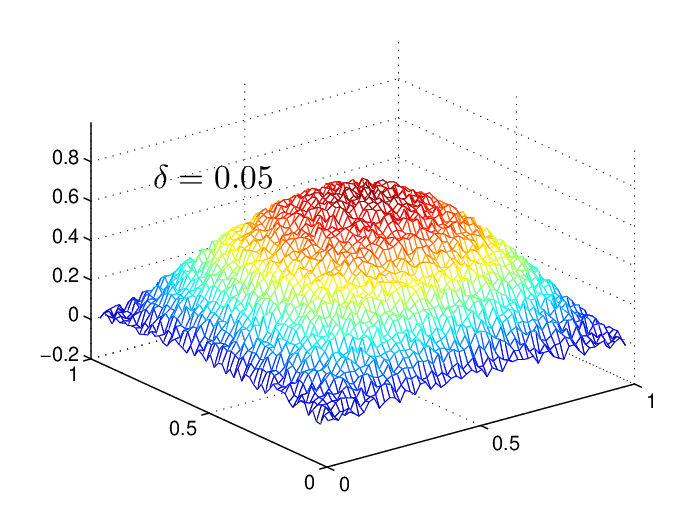
In our computation, the noisy data $y_{\delta}$ is generated by adding a random noise to the observation data $y$:

$$y_{\delta}(x)=y(x)+\mbox{rand}(x),$$

where rand($x$) is a uniformly distributed random function in $[-1,1]$, and $\delta$ is the noise level. The unknown source (exact solution) $u$ and the noise free data $y$ are depicted in the first row of Fig. 4.

References

- [1] G. Allaire, Shape optimization by the homogenization method, Springer-Verlag, New York, 2002.
- [2] D. P. Bertsekas, Augmented Lagrangian and differentiable exact penalty methods, in Nonlinear optimization, 1981 (Cambridge, 1981), NATO Conf. Ser. II: Systems Sci., Academic Press, London, (1982), pp. 223–234.
- [3] D. P. Bertsekas, Constrained optimization and Lagrange multiplier methods, Academic Press Inc, New York, 1982.
- [4] K. D. Bhalerao, C. Crean, and K. Anderson, Hybrid complementarity formulations for robotics applications, ZAMM Z. Angew. Math. Mech., 91 (2011), pp. 386–399.
- [5] J. F. Bonnans, Numerical optimization: theoretical and practical aspects, Springer-Verlag New York Inc, 2006.
- [6] J. F. Bonnans, J. C. Gilbert, C. Lemaréchal, and C. A. Sagastizábal, Numerical optimization, Springer-Verlag, Berlin, second ed., 2006.
- [7] D. Boukari and A. V. Fiacco, Survey of penalty, exact-penalty and multiplier methods from 1968 to 1993, Optimization, 32 (1995), pp. 301–334.
- [8] R. H. Byrd, J. Nocedal, and R. A. Waltz, Steering exact penalty methods for nonlinear programming, Optim. Methods Softw., 23 (2008), pp. 197–213.
- [9] A. R. Conn and T. Pietrzykowski, A penalty function method converging directly to a constrained optimum, SIAM J. Numer. Anal., 14 (1977), pp. 348–375.
- [10] G. D. Pillo, Exact penalty methods, in Algorithms for continuous optimization (Il Ciocco, 1993), vol. 434 of NATO Adv. Sci. Inst. Ser. C Math. Phys. Sci., Kluwer Acad. Publ., Dordrecht, 1994, pp. 209–253.
- [11] R. Glowinski, Numerical methods for nonlinear variational problems, Springer-Verlag, Berlin, 2008.
- [12] R. Glowinski, J. L. Lions, and R. Trémolières, Numerical analysis of variational inequalities, North-Holland Publishing Co., Amsterdam, 1981.
- [13] W. W. Hager and H. Zhang, A new active set algorithm for box constrained optimization, SIAM J. Optim., 17 (2006), pp. 526–557.
- [14] S. P. Han, A globally convergent method for nonlinear programming, J. Optimization Theory Appl., 22 (1977), pp. 297–309.
- [15] B. Hassani and E. Hinton, Homogenization and structural topology optimization, Springer-Verlag, London, 1999.
- [16] P. Hild and P. Laborde, Quadratic finite element methods for unilateral contact problems, Applied Numerical Mathematics, 41 (2002), pp. 401 – 421.
- [17] M. Hintermüller, V. A. Kovtunenko, and K. Kunisch, Obstacle problems with cohesion: a hemivariational inequality approach and its efficient numerical solution, SIAM J. Optim., 21 (2011), pp. 491–516.
- [18] R. H. W. Hoppe and R. Kornhuber, Adaptive multilevel methods for obstacle problems, SIAM J. Numer. Anal., 31 (1994), pp. 301–323.
- [19] K. Ito, B. Jin, and T. Takeuchi, Multi-parameter Tikhonov regularization, Methods Appl. Anal., 18 (2011), pp. 31–46.
- [20] K. Ito, B. Jin, and T. Takeuchi, A regularization parameter for nonsmooth Tikhonov regularization, SIAM J. Sci. Comput., 33 (2011), pp. 1415–1438.
- [21] K. Ito and K. Kunisch, Optimal control of obstacle problems by -obstacles, Appl. Math. Optim., 56 (2007), pp. 1–17.
- [22] K. Ito and K. Kunisch, Lagrange multiplier approach to variational problems and applications, SIAM, Philadelphia, 2008.
- [23] N. Kikuchi and J. T. Oden, Contact problems in elasticity: a study of variational inequalities and finite element methods, vol. 8 of SIAM Studies in Applied Mathematics, Society for Industrial and Applied Mathematics (SIAM), Philadelphia, 1988.
- [24] M. A. Noor and S.I.A. Tirmiz, Finite difference technique for solving obstacle problems, Applied Mathematics Letters, 1 (1988), pp. 267 – 271.
- [25] R. Scholz, Numerical solution of the obstacle problem by the penalty method, Computing, 32 (1984), pp. 297–306.
- [26] O. Sigmund, Morphology-based black and white filters for topology optimization, Structural and Multidisciplinary Optimization, 33 (2007), pp. 401–424.
- [27] D. E. Stewart, Finite-dimensional contact mechanics, R. Soc. Lond. Philos. Trans. Ser. A Math. Phys. Eng. Sci., 359 (2001), pp. 2467–2482.
- [28] J. Toivanen and C. W. Oosterlee, A projected algebraic multigrid method for linear complementarity problems, Numer. Math. Theory Methods Appl., 5 (2012), pp. 85–98.
- [29] X. S. Zhang, Neural networks in optimization, Kluwer Academic Publishers, Dordrecht, 2000.