The faster the narrower: characteristic bulk velocities and jet opening angles of Gamma Ray Bursts
Abstract
The jet opening angle and the bulk Lorentz factor are crucial parameters for the computation of the energetics of Gamma Ray Bursts (GRBs). From the 30 GRBs with measured or it is known that: (i) the real energetic , obtained by correcting the isotropic equivalent energy for the collimation factor , is clustered around – erg and it is correlated with the peak energy of the prompt emission and (ii) the comoving frame and are clustered around typical values. Current estimates of and are based on incomplete data samples and their observed distributions could be subject to biases. Through a population synthesis code we investigate whether different assumed intrinsic distributions of and can reproduce a set of observational constraints Assuming that all bursts have the same and in the comoving frame, we find that and cannot be distributed as single power–laws. The best agreement between our simulation and the available data is obtained assuming (a) log–normal distributions for and and (b) an intrinsic relation between the peak values of their distributions, i.e 2.5=const. On average, larger values of (i.e. the “faster” bursts) correspond to smaller values of (i.e. the “narrower”). We predict that 6% of the bursts that point to us should not show any jet break in their afterglow light curve since they have . Finally, we estimate that the local rate of GRBs is 0.3% of all local SNIb/c and 4.3% of local hypernovae, i.e. SNIb/c with broad–lines.
Keywords:
Gamma-ray: bursts1 Introduction
Gamma Ray Bursts (GRBs) have extremely high energetics. The isotropic equivalent energy , released during the prompt phase, is distributed over four orders of magnitudes in the range 1050-54 erg. correlates with , i.e. the peak of the spectrum (Amati et al. 2002, 2009): . This holds for long duration GRBs. A similar correlation exists between the isotropic equivalent luminosity and (Yonetoku et al. 2004) obeyed also by short events (Ghirlanda et al. 2009). The scatter of the data points around the correlation, modeled with a Gaussian, has a dispersion 0.23 dex (see e.g. Nava et al. 2012 for a recent update of these correlations). This dispersion is much larger than the average statistical error dex and dex associated with and , respectively.
Since is computed assuming that GRBs emit isotropically, it is only a proxy of the real GRB energetic. GRBs are thought to emit their radiation within a jet of opening angle . If the jet opening angle is known, the true energy and the true GRB rate can be estimated (Frail et al. 2001).
The estimate of is made possible by the measure of the jet break time , typically observed between 0.1 to 10 days in the afterglow optical light curve. Although has been measured only for 30 GRBs (Ghirlanda et al. 2007) it shows that:
- 1.
clusters around erg with a small dispersion (Frail et al. 2001; but see Racusin et al. 2009; Kocevski & Butler 2008);
- 2.
is tightly correlated with (Ghirlanda, Ghisellini & Lazzati 2004; Ghirlanda et al. 2007) with a scatter dex (consistent with the average statistical error dex associated with and );
- 3.
the true rate of local GRBs ranges from 250 Gpc-3 yr-1 (e.g. Frail et al. 2001) to 33 Gpc-3 yr-1 (Guetta, Piran & Waxman 2005). These different values are mainly due to the different values assumed for the collimation factor . The true GRB rate can be compared with the local rate of SN Ib/c (e.g. Soderberg 2006; Guetta & Della Valle 2007; Grieco et al. 2012), i.e. the candidate progenitors of long GRBs, and allows to estimate the rate of orphan afterglows (e.g. Guetta et al. 2005).
The , and correlations could enclose some underlying feature of the GRB emission mechanism (e.g. Rees & Meszaros 2005; Ryde et al. 2006; Thompson 2006; Giannios & Spruit 2007; Thompson, Meszaros & Rees 2007; Panaitescu 2009), of the GRB jet structure (e.g. Yamazaki, Ioka & Nakamura 2004; Eichler & Levinson 2005; Lamb, Donaghy & Graziani 2005; Levinson & Eichler 2005) or of the progenitor (e.g. Lazzati, Morsony & Begelman 2011). An intriguing application of these correlations is the use of GRBs as standard candles (Ghirlanda, Ghisellini & Firmani 2005; Firmani et al. 2005; Amati et al. 2009).
The presence of outliers of the correlation in the CGRO/BATSE GRB population (Band & Preece 2005; Nakar & Piran 2005; Shahmoradi & Nemiroff 2011) and in the Fermi/GBM burst sample (Collazzi et al. 2012) and the presence of possible instrumental biases (Butler et al. 2007; Butler, Kocevski & Bloom 2009; Kocevski 2012) caution about the use of these correlations either for deepening into the physics of GRBs and for cosmological purposes. Although instrumental selection effects are present, it seems that they cannot produce the correlations we see (Ghirlanda et al. 2008; Nava et al. 2008; Ghirlanda et al. 2012b). Moreover, a correlation between and is present within individual GRBs as a function of time (Firmani et al. 2009; Ghirlanda et al. 2010; 2011; 2011a), suggesting that the radiative process(es) might be the origin of the correlation. Despite these studies, the spectral energy correlations of GRBs and their possible applications are still a matter of intense debate.
A new piece of information recently added to the puzzle is that the GRB energetics (, and ) appear nearly similar in the comoving frame (Ghirlanda et al. 2012 -- G12 hereafter). To measure these comoving quantities11 1 Primed quantities are in the comoving frame of the source. we have to know the bulk Lorentz factor , that can be estimated through the measurement of the peak time of the afterglow light curve. G12 could estimate in 30 long GRBs with known and well defined energetics, finding that:
- 1.
() and ;
- 2.
the comoving frame 3.5 erg (dispersion 0.45 dex), 5 erg s-1 (dispersion 0.23 dex) and 6 keV (dispersion 0.27 dex).
These results imply that the and correlation are a sequence of different factors (see also Dado, Dar & De Rujula 2007).
The values of GRBs are known only for a couple of dozens of bursts (Ghirlanda et al. 2007). appears distributed as a log–normal with a typical (Ghirlanda et al. 2005). By correcting the isotropic comoving frame energy by this typical jet opening angle, the comoving frame true energy results erg. In G12 we also argued that in order to have consistency between the and the correlations one must require = constant. A possible anti–correlation between and is predicted by models of magnetically accelerated jets (Tchekhovskoy, McKinney & Narayan 2009; Komissarov, Vlahakis & Koenigl 2010) but, at present, only 4 GRBs have an estimate of and and well constrained spectral properties.
The measure of relies on the measure of , that in turn requires the follow up of the optical afterglow emission up to a few days after the burst explosion (Ghirlanda et al. 2007). The measurement of is difficult, not only because it requires a large investment of telescope time, but also because several are chromatic (contrary to what predicted; but see Ghisellini et al. 2009), and the jet break can be a smooth transition whose measurement requires an excellent sampling of the afterglow light curve (e.g. Van Eerten et al. 2010, 2011). Another complication is that the early afterglow emission is characterized by several breaks. For instance, the end of the plateaux phase typically observed in the X–ray light curves, if misinterpreted as a jet break, biases the distribution towards small values of (Nava, Ghisellini & Ghirlanda 2006). Finally, the measure of large is complicated by the faintness of the afterglow and its possible contamination by the host galaxy emission and the supernova associated to the burst. Several observational biases could shape the observed distribution. Among these the fact that more luminous bursts (i.e. those more easily detected) should have the smallest jet opening angles. For all these reasons the observed distribution of might not be representative of the real distribution of GRBs jet opening angles.
The distribution of is centered around =65 (130) in the case of a wind (uniform) density distribution of the circum–burst medium. The distribution of is broad and extends between 20 and 800. These results are still based on a sample of only 30 GRBs (G12). The difficulties of early follow–up of the optical afterglow emission could prevent the measure of very large on the one hand, while the possible contamination by flares (Burrows et al. 2005; Falcone et al. 2007) or by other (non afterglow) emission components (e.g. Ghisellini et al. 2010) at intermediate times could prevent the estimate of the low–end of the distribution. One could argue if GRBs can have of a few. While there are some hints that GRB060218 should have 5 (Ghisellini et al. 2006) the classical compactness argument, for typical GRB parameters (e.g. Piran 1999), requires that 100-200. This argument was successfully applied to few bursts observed up to GeV energies by LAT on board Fermi (e.g. Abdo et al. 2009, Ghirlanda et al. 2009) to derive lower limits of several hundreds on . If, instead, the highest energy photon detected has an energy of say MeV, the lower limit derived from the classical compactness argument would be a few (i.e. ). Therefore, also in the case of , the observed distribution, derived with still few events, could be not representative of the real distribution of this parameter.
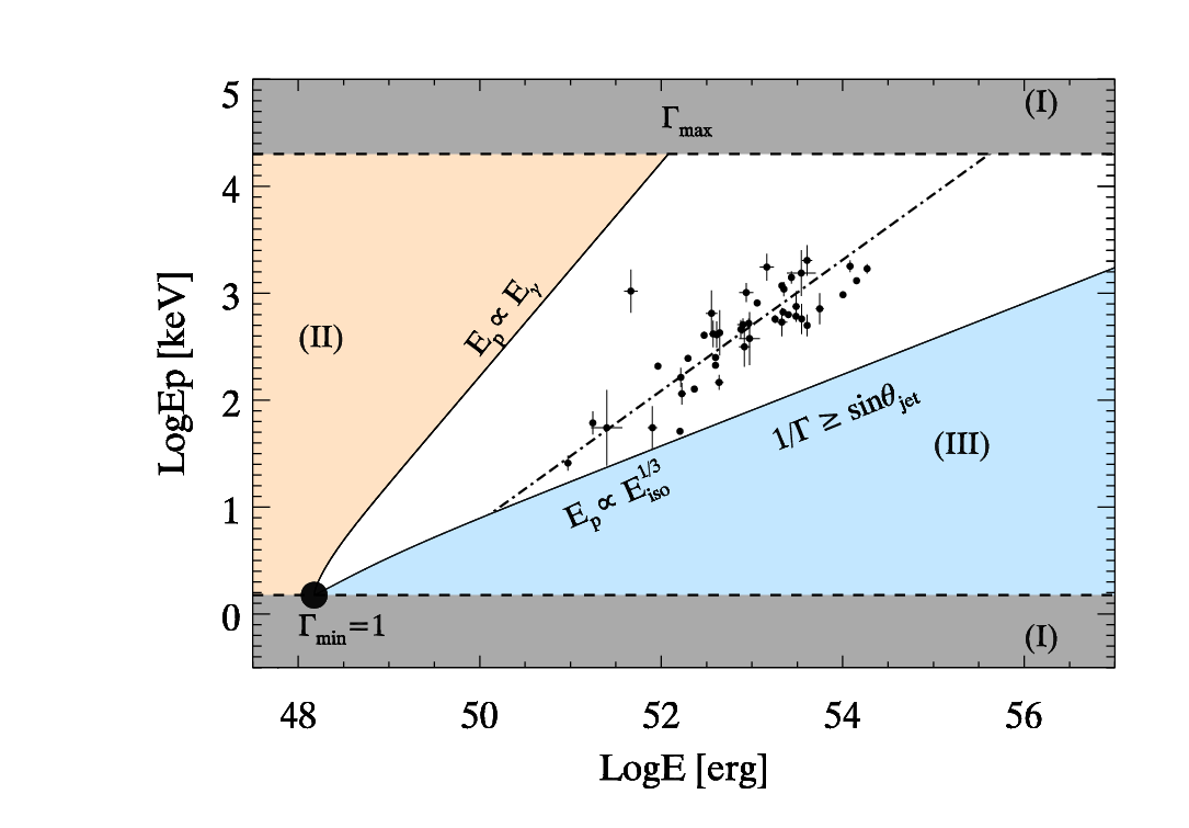
The main aim of this paper is to constrain the distribution of and in GRBs using the available independent constraints. This aim can be translated into a simple question: do and follow power law distributions or do they follow some kind of peaked distribution (e.g. a broken power law or a log–normal)? In both cases the resulting distributions could be different from the observed ones since some selection effect (as discussed above) might prevent to measure very low and/or high values of and . Another scope of the present paper is to test which is (if any) the relation between and . A relation 2=const was assumed in G12 to explain the spectral energy correlations and a similar relation seems to arise from numerical simulations of jet accelerations (Tcheckolskoy et al. 2012). Here we use several observational constraints and test whether there is a a=const relation and try to constrain its exponent . One important effect that we consider in this paper for the first time is the collimation of the burst radiation when is small. In general we are led to think that given a value of the collimation corrected energy , the corresponding isotropic equivalent energy is /2. This is true if the beaming of the radiation is “dominated” by the jet opening angle, i.e. 1/. However, GRBs with very low could have 1/ and in this case the isotropic equivalent energy is determined by (i.e. 2 - see §. 2.2) rather than by . This effect, introduces a limit (1/3) in the classical plane (Fig.1) accounting for the absence of bursts with intermediate/low and large values of . This limit can also partly account for the problem of “missing jet breaks” since these bursts with 1/ should not show any jet break in their afterglow light curve (§4.5).
We rely on a GRB population synthesis code that we have recently adopted to explore the issue of instrumental selection biases on the correlation (Ghirlanda et al. 2012b).
The simulation steps are described in §2 while the observational constraints that we aim to reproduce are outlined in §3. In §4 we present our results. We summarize and discuss our findings in §5. Throughout the paper a standard flat universe with is assumed.
2 Population synthesis code
So far, the approach adopted in studying the spectral–energy correlations and the distributions of or was (i) to derive the collimation corrected correlation by correcting the isotropic energy for the collimation factor (e.g. Ghirlanda et al. 2004), or (ii) to derive the comoving frame properties of GRBs by correcting, for the factor, the isotropic values , and (G12).
In this paper, we tackle the problem from the opposite side and jointly work with and : we assume that GRBs have all the same comoving frame and and simulate GRB samples with different distributions of and . This produces a population of GRBs with known energetics , peak energy and observer frame fluence and peak flux . We would like to stress that our main assumption (same and for all burst) is a crude simplification. Nevertheless, our assumption can work if the real and distributions are indeed narrower that the distributions of the corresponding observed quantities. Recently, Giannios 2012 have shown that in photospheric models a comoving frame peak energy 1.5 keV is expected.
The observational constraints that we aim to reproduce (see §3) are: (i) the rate of GRBs observed by Swift/BAT, CGRO/BATSE and Fermi/GBM, (ii) the correlation defined by the complete sample of Swift bright bursts (Salvaterra et al. 2012; Nava et al. 2012) and (iii) the fluence and peak flux distributions of the population of bursts detected by Fermi/GBM (Goldstein et al. 2012) and CGRO/BATSE (Meegan et al. 1998).
Note that, since one of the aims of the present paper is to constrain the distributions of and we cannot adopt the observed ones (discussed in the introduction) as constraints, otherwise we would fall into a circular argument. The distributions of and that we assume in our simulations (power law, broken power law, log–normal) have all their characteristic parameters (slope, normalization, break values, width etc.) free to vary. These parameters are what we aim to constrain through our population synthesis code.
In Fig. 1 we show the rest frame peak energy versus the total energy (where here is generically used to indicate an energy, either isotropic or collimation corrected). We highlight different regions (I, II and III) that are useful to explain the simulation steps (§2.1). This plane will be one of our observational constraints: in Fig. 1 we show (black filled points) the Swift complete sample of bursts (Salvaterra et al. 2012; Nava et al. 2012) which we aim to reproduce through our simulations.
2.1 Simulation steps
Our starting assumption is that all GRBs have the same comoving frame =1.5 keV and =1.5 erg. This is shown by the black circle in Fig. 1. G12 find that const and that the observed duration does not depend on . Therefore, in the comoving frame, . It follows that = is also constant if, as discussed in G12, =const. Although some dispersion of the values of is present in the sample of G12, the value of that we assume here is consistent at the 2 level of confidence with the distribution of values reported in G12 for the wind density ISM.
The main steps of our simulation are:
- 1.
we simulate a population of GRBs distributed in redshift between and according to the GRB formation rate (GRBFR) . This is formed by two parts: . The first term is a cosmic evolution term, while is taken from Li (2008) (which extended to higher redshifts the results of Hopkins & Beacom 2008):
(1) is in units of . Concerning , Salvaterra et al. (2012) derived the luminosity function of GRBs by jointly fitting the redshift distribution of a complete sample of bright GRBs detected by Swift and the count distribution of a larger sample of BATSE bursts. They found that either the evolution of the luminosity function or the evolution of the density of GRBs is required in order to account for these data sets. We assume the same term found by S12.
- 2.
We assign to each GRB a bulk Lorentz factor extracted from a specified distribution, in the range [1, 8000]. The upper limit () is somewhat arbitrary, but large enough to encompass all the values of estimated so far, and in particular the large values derived for the few GRBs detected by the LAT instrument on board Fermi, if the GeV emission is interpreted as afterglow (Ghisellini et al. 2010).
For each simulated burst the rest frame peak energy and the energy are (see G12):
(2) where =. The simulated bursts define a correlation between and :
(3) for this corresponds to the correlation in the case of a wind density profile (Nava et al. 2006). This relation is shown in Fig. 1 with the solid black line (labelled ). The simulated distribute between 1.5 keV (=1) and 20 MeV (=8000).
- 3.
We assign to each simulated burst a jet opening angle extracted from a specified distribution.
- 4.
The probability for a burst to be observed from the Earth depends on the viewing angle between the jet axis and the line of sight of the observer. We extract randomly a viewing angle from the cumulative distribution of the probability density function .
- 5.
In order to compare the simulated bursts with the source count distribution of existing samples of GRBs (see §3) we compute the observer frame peak fluxes and fluences . To this aim we assume a typical spectrum described by the Band function (Band et al. 1993), with low and high photon spectral indexes and , respectively (i.e. corresponding to the typical values observed by different instruments -- e.g. Kaneko et al. 2006; Sakamoto et al. 2011)22 2 These values are also assumed by S12 to constrain the LF of GRBs.. The fluence of each simulated burst in a given energy range is computed by re-normalizing this spectrum through the bolometric fluence =, where is the luminosity distance for a given redshift . To derive the peak flux , we assign to each burst an (observer frame) duration extracted from a distribution centered at 27.5 s and with a dispersion . This distribution is truncated at s because we consider only long duration GRBs in this analysis. Such a duration distribution is similar to that of the Fermi/GBM GRBs (Paciesas et al. 2012; Goldstein et al. 2012) and includes also very long bursts with 300 s. We assume that the bursts have a simple triangular light curve and derive the peak luminosity as . The peak flux in a given energy range is obtained by re–normalizing the spectrum through the bolometric peak flux .
2.2 Computation of
The isotropic equivalent energy of the simulated bursts can be derived from . Since 90∘, simulated bursts cannot be in region II of Fig. 1 and can take values on the right hand side of the limit of Eq. 3 shown in Fig. 1. According to the values of and assigned to each simulated bursts, the isotropic equivalent energy is:
| (4) |
| (5) |
In the latter case is smaller than in Eq. 4. This introduces a limit in the plane of Fig. 1 corresponding to the line:
| (6) |
(labelled 1/3 in Fig. 1). For a given , bursts with a small value of will have an computed through Eq. 5 and will lie on the limiting line of region III in Fig. 1. Their radiation is, indeed, collimated within an angle (1/) which is larger than their .
Simulated bursts can populate the region delimited by boundaries (I, II and III) in Fig. 1. This is one (among others) observational constraint that we will adopt in our simulations (§3) to constrain the distributions of and and their possible relation. According to the relative values of , and , simulated bursts are classified as: bursts “pointing to us” (PO, hereafter), i.e. those that can be seen from the Earth, with max[, 1/] and bursts pointing in other directions (NPO, hereafter), i.e. not observable from the Earth, with max[, 1/]. We will compare the PO simulated bursts with our observational constraints, while the entire population of simulated bursts (i.e. PO and NPO) will be used to infer the properties of GRBs (e.g. the distributions of and and the true burst rate).
3 Observational constraints
In order to test whether and assume characteristic values or not we compare the population of simulated bursts with real samples of GRBs. In this section we describe our observational constraints. We consider the ensemble of GRBs detected by the Burst Alert Telescope (BAT) on board Swift, the Gamma Burst Monitor (GBM) on board Fermi and the Burst And Transient Source Experiment (BATSE) on board the Compton Gamma Ray Observatory (CGRO).
3.1 The Swift BAT complete sample
Salvaterra et al. (2012 - S12 hereafter) constructed a sample of bright Swift bursts consisting of 58 GRBs detected by Swift/BAT with =2.6 ph cm-2 s-1 (integrated in the 15–150 keV energy range). Fifty four of these events have a measured redshift so that the S12 sample is 90% complete in redshift. Forty six (out of 54) GRBs in this sample have well determined spectral properties (filled circles in Fig. 1) and define a statistically robust correlation with rank correlation coefficient and chance probability (Nava et al. 2012, N12 hereafter)33 3 The 8 GRBs without a secure estimate of the redshift or with incomplete spectral informations are consistent with the correlation defined by the 46 GRBs discussed here, see N12 for details.. The correlation properties (slope and normalization) of the complete Swift sample are consistent with those defined with the incomplete larger sample of 136 bursts with known and spectral parameters (see N12). Therefore, the distribution of the Swift complete sample (46/54 events with well constrained ) in the plane is representative of the larger (heterogeneous) population of GRBs with measured and well constrained spectral properties. The 46 GRBs of the complete Swift sample define a correlation (shown by the dot–dashed line in Fig. 1) with a scatter (computed perpendicular to the best fit line) with a Gaussian dispersion 0.29 dex.
The Swift complete sample of S12 contains 1/3 of the bursts detected by Swift44 4 http://swift.gsfc.nasa.gov/docs/swift/archive/grb_table/ with 2.6 ph cm-2 s-1. We verified that the Swift complete sample of 54 events selected by S12 is representative of the larger population of 149 long Swift bursts with : the Kolmogorov–Smirnov test on the peak flux distribution of the two samples gives a probability of 0.6 that the two distributions are drawn from the same parent population. These bursts were not included in the selection of S12 because they do not have favorable conditions for ground–based follow up.
These 149 events with are the bursts detected by Swift in 7 yrs from its launch within the (half coded) field of view of 1.4 sr of BAT. This corresponds to an average Swift detection rate of 15 events sr-1 yr-1.
3.2 The Fermi GBM sample
Another observational constraint that we consider is the population of bursts detected by the GBM on board Fermi. The spectral properties of GBM bursts have been studied in Nava et al. (2011a) and compared to those of BATSE bursts in Nava et al. (2011b). More recently, the first release of the GBM spectral catalog (Goldstein et al. 2012) provided the spectral parameters and derived quantities (i.e. peak fluxes and fluences) for 487 GRBs detected by the GBM in its first 2 years of activity. 398 bursts in this catalog are long events and have measured peak flux and fluence (both integrated in the 10 keV--1 MeV energy range)55 5 and are reported in Goldstein et al. (2012) and were obtained by integrating the model that best fits the peak time resolved spectrum and the time averaged spectrum, respectively..
We cut the GBM sample to ph cm-2 s-1, in order to account for the possible incompleteness of the sample at lower fluxes, obtaining 312 GBM bursts.
The GBM is an all sky monitor that observes on average 60–70% of the sky. Therefore, the average GBM detection rate is 21 events sr-1 yr-1 with peak flux, integrated in the 10 keV–1 MeV energy range, ph cm-2 s-1.
3.3 The CGRO BATSE sample
We also consider the sample of GRBs detected by BATSE. The 4B sample (Meegan et al. 1998) contains 1540 long events and 1496 of these have their and (both integrated in the 50–300 keV energy range) measured. The sample of 1496 BATSE bursts is cut at ph cm-2 s-1 with 716 BATSE bursts above this threshold. Considering the average portion of the sky observed by BATSE, i.e. 70% of the sky, the detection rate of BATSE is 16 events sr-1 yr-1 for GRBs with a peak flux, integrated in the 50–300 keV energy range, 1 ph cm-2 s-1.
The lower detection rate of BATSE with respect to GBM is due to the different energy range where the peak fluxes are calculated (i.e. 10 keV–1 MeV for GBM and 50–300 keV for BATSE, respectively). We verified that by considering the GBM bursts with peak flux integrated in the same energy range of BATSE (i.e. 50–300 keV) larger than 1 ph cm-2 s-1 (i.e. the same threshold adopted for BATSE), the GBM rate is equal to the BATSE one.
3.4 Extraction of results
From each simulation we extract three populations of GRBs among the bursts pointing to us (PO):
- 1.
the Swift comparison sample: simulated GRBs with peak flux, integrated in the 15–150 keV band, larger than 2.6 ph cm-2 s-1. We also require that their observer frame peak energy is in the range 15 keV–2 MeV. Indeed, this is the energy range where can be measured by presently flying satellites like Swift, Konus and Fermi.
- 2.
the GBM comparison sample: simulated bursts with a peak flux, integrated in the 10 keV–1 MeV energy range, larger than 2.5 ph cm-2 s-1;
- 3.
the BATSE comparison sample: simulated bursts with a peak flux, integrated in the 50–300 keV energy range, larger than 1.0 ph cm-2 s-1.
The simulation is adjusted so that the Swift comparison sample contains 149 GRBs, i.e. the same number of bright bursts detected by Swift (§3.1). Therefore, the Swift rate is imposed. What we derive instead from the simulation is the rate of GBM and BATSE GRBs that we compare with the real rates of these two instruments described in §3.2 and §3.3 respectively.
We also require that the Swift comparison sample is consistent with the Swift complete sample of S12. To this aim we compare them in the rest frame plane and in the observer frame plane deriving a 2 dimensional Kolmogorov–Smirnov (KS) probability (one for the and one for plane). We also verify through a 1 dimensional KS test that the redshift distribution of the Swift comparison sample is consistent with that of the Swift complete sample. Finally we compare, through a 1D–KS test, the fluence and peak flux distributions of the GBM and BATSE comparison samples with those of the real samples of GRBs detected by these instruments and described in §3.2 and §3.3, respectively.
Since the Swift complete sample contains only the brightest Swift bursts it maps the high end of the peak flux distribution of GRBs. The GBM and BATSE samples that we adopt here extend the comparison sample to lower values of and ensures that our simulations reproduce also the faint end of the GRB population66 6 The values of the GBM sample are computed on the broad 10 keV–1 MeV energy range (i.e. much broader than the 15–150 keV energy range of Swift). This ensures that the selected sample of the GBM bursts extends the population of GRBs to lower fluxes than those of the Swift complete sample..
For each simulation we derive the following probabilities:
- •
the 2D-KS probability that the Swift comparison sample is consistent with the complete Swift sample of S12 in the plane;
- •
the 2D-KS probability that the Swift comparison sample is consistent with the complete Swift sample of S12 in the plane;
- •
the 1D-KS probability that the Swift comparison sample has a redshift distribution consistent with that of the S12 Swift sample;
- •
the 1D-KS probabilities that the GBM comparison sample is consistent with the GBM sample in terms of peak flux and fluence ;
- •
the 1D-KS probabilities that the BATSE comparison sample is consistent with the BATSE sample in terms of peak flux and fluence ;
- •
we verify if the GBM rate predicted by the simulation is consistent, at 1, with the GBM rate .
- •
we verify if the BATSE rate predicted by the simulation is consistent, at 1, with the BATSE rate .
For the KS probabilities we set a limit of 10-3 below which we consider that two distributions (either 1D or 2D) are inconsistent at more than 3. Each simulation, with its assumptions on the distribution of and , is repeated 1000 times and we compute the percentage of repeated simulations that produce GRB samples (i.e. Swift, GBM and BATSE comparison samples) consistent with our observational constraints.
4 Results
In the following sections we present the results obtained with different possible assumptions for the distributions of and . We want to test which one among the possible intrinsic distributions of and that one can think of (e.g. power laws, broken power laws or log–normal) best reproduces the observational constraints described in the previous section.
4.1 Power law distributions of and
We assume that both and are distributed as power laws: and . This corresponds to the hypothesis that and do not have a characteristic value. We consider and .
The choice of these parameters corresponds to have most of the simulated bursts with low factors and with small values. One could think that such distributions are already excluded by the observed distributions of and (which are log–normal) discussed in §1. However, those are the observed distributions of and and they are subject to several biases (see §1). The intrinsic distributions might well be completely different and this motivates to start with this simplest assumption, i.e. that both and have power law distributions.
Under the hypothesis that both and have power law distributions (with free parameters and varied in the above ranges with a step 0.2 in both parameters), only in 1% of 1000 repeated simulations we can find an agreement with all our observational constraints. In order to show the inconsistency of the simulations with the observational constraints we present in Fig. 2 the results of the simulations assuming that and have power law distributions with . This case, shown as an example, corresponds to a uniform distribution of Log and Log.
The rest frame plane (top left panel in Fig. 2) is filled uniformly with simulated bursts (yellow dots) distributed between the limit and with a minimum =1∘ (the oblique right limit to the distribution of yellow dots). The simulated GRBs pointing to us (PO) have preferentially large values (blue dots in the top left panel of Fig. 2). The simulated bursts of the Swift comparison sample (here represented by the smoothed density contours77 7 These are obtained by staking 1000 simulations and smoothing the obtained distribution in the plane. – red solid lines in Fig. 2) are inconsistent with the real GRBs of the Swift complete sample (open squares). The red contours extend at high values where there is a deficit of Swift bursts and they also over predict the number of bursts on the right hand side of the distribution of the real Swift bursts (i.e towards large values of for intermediate/high values of ).
Also in the observer frame plane (top right panel in Fig. 2) the simulated Swift comparison sample (solid contours) are inconsistent with the real Swift bursts of the complete sample (open squares). Simulated bursts of the Swift comparison sample tend to concentrate towards the upper part of the plane.
The bottom panels of Fig. 2 show the cumulative rate distribution of the fluence for the GBM and BATSE sample (right and left panels of Fig. 2) compared with the predictions of the simulations (dashed regions in the bottom panels of Fig. 2). The rate of GBM and BATSE bursts predicted by the simulation which assumes a power law distribution for both and (with index –1) is a factor 2 larger than the rate of GBM bursts. Also the distributions of the peak flux of the simulated BATSE and GBM samples are inconsistent with the real samples.
If we assume steeper power law distributions of and [e.g. ], the excess of bursts with large peak energy (both in the rest frame and in the observer frame of Fig. 2, top left and right panels respectively) is reduced but the rate of simulated GBM and BATSE bursts increases becoming more inconsistent with the real rates of GRBs detected by these two instruments (bottom panels of Fig. 2). This result shows that all the constraints that we have adopted (§3) are relevant: the GBM and BATSE comparison sample map the low end of the peak flux/fluence distribution while the Swift complete sample maps the bright burst tail of such distributions. The bursts of the Swift complete sample, having their measured, map the distribution of GRBs in the rest frame plane.
4.2 Peaked distributions of and
Since we could not find agreement between the simulations which assume power law distributions of and and our observational constraints, we now consider the case of peaked distributions of and .
The simplest assumption is that and/or are distributed as broken power laws. We first assumed that only or have a broken power law distribution, while the other parameter is distributed as a single power law. In this case we cannot find a percentage of repeated simulations larger than 2% in agreement with our observational constraints.
We then considered the case of a broken power law distribution for both and :
For the distribution of we consider the following parameter ranges: , and . For : , and . The free parameters are varied with step 0.1 for and and 0.5∘ for for the broken power law distribution of and with step 0.1 for and and 10 for for the broken power law distribution of .
We find that at most 20% of the 1000 repeated simulations reproduce our observational constraints when and with step 0.1 for and and 10 for for the broken power law distribution of . A lower percentage of agreement is obtained for any other choice of the free parameters.
We show in Fig. 3 the results of the simulations with the above parameter values for the distributions of and . We note that a better agreement is now found between the rate of the GBM and BATSE bursts (bottom panels of Fig. 3) while the distribution of simulated bursts of the Swift comparison sample (solid contours) are inconsistent with the Swift bursts of the complete sample both in the rest frame plane (top left panel of Fig. 3) and in the observer frame plane (top right panel of Fig. 3).
The assumption of a characteristic value of corresponds to concentrate GRBs around a typical value of (see Eq. 2). In this case the narrower distribution reduces the number of simulated bursts with large values of , thus clustering the simulated GRBs of the PO class around the limit of Fig. 3 (top left panel) that was found in the case of single power laws (§4.1).
A broken power law is a simple approximation of a peaked distribution. The real distribution of and could have a different shape. We then considered the case of log–normal distributions for both and , with central values of the distribution between 3∘ and 12∘ (step 0.5∘) and width between 0.3 and 0.8 (step 0.05) and central values of between 50 and 120 (step 5) and width between 0.2 and 0.8 (step 0.05). We find that, if has a log–normal distribution with a median value of 4.5∘ (with a dispersion of 0.5) and is distributed as a log–normal with median 85 (with a dispersion of 0.45), the 40% of the 1000 repeated simulations is in agreement with all our observational constraints.
The latter assumption, that seems to improve the consistency between the simulated GRB population and the observational constraints, suggests that and have log–normal distributions. However, the fact that no more than 40% of the repeated simulations can reproduce all our observational constraints, is suggesting that some ingredient is still missing. This is the subject of the next section where we study for the first time through our numerical simulations, the possibility that there is a relation between the average values of and .
4.3 The relation between and
By assuming a distribution with a characteristic value as in §4.2, the simulated bursts in the plane cluster around a correlation which is linear in this plane (i.e. parallel to the limit), while the correlation defined by the Swift complete sample (and similarly by the larger, incomplete, sample of bursts with measured redshift – see N12) has a flatter slope, i.e. . In other words, for an infinitely narrow distribution of , the simulated bursts (yellow dots in Fig. 3 top left panel) would produce a linear correlation which is inconsistent with the observed correlation. This suggests that, besides the fact that and should have characteristic values (i.e. peaked distributions), they should also be correlated.
Indeed, G12 find that the comoving frame properties of GRBs (and in particular the fact that and 2) can be combined to explain both the and the correlation if the ansatz 2=const is valid. Several recent numerical simulations of jet acceleration in GRBs suggest that a link between and should exist, although the form of this relation depends on several assumptions of these simulations. In this section we explore, for the first time, if a relation m= can account for the observational constraints described in §3 and in this case we constrain its free parameters ( and ). We start from the result of the previous section, which showed that the best result (i.e. 40% of the repeated simulations are in agreement with the observations) is obtained assuming two log–normal distributions for and .
We simulate bursts with Log distributed as a Gaussians with a characteristic central value Log and a dispersion . Similarly we assume a Gaussian distribution for Log centered at Log and with a dispersion . We then assume that there is a relation between and of the form LogLog. In this way the distribution of Log is centered on a value which is given by the assumed relation between and .
We explored the parameter space (defined by 5 free parameters) and found that 80% of our simulations are consistent with our constraints if Log with a dispersion of dex, , and dex.
We show in Fig. 4 the results of this simulation which assumes log–normal distributions of and and a relation between these two parameters. In the plane (top left panel in Fig. 4) and in the plane (top right in Fig. 4) we find a good agreement between the simulated Swift comparison sample (solid contours) and the real Swift complete sample (open squares). Now the predicted rate of GBM and BATSE bursts is fully consistent with the real ones (bottom left and right panels in Fig. 4 respectively).
We stress that, given the assumptions of our simulation (e.g. the spectrum, duration and unique values of the comoving frame energetics of all GRBs) we do not expect to find 100% of the simulations reproducing our constraints. However, we can use our code to derive interesting properties of the population of GRBs. Indeed, in our simulations we generate a population of GRBs pointing in every direction. Only those pointing towards the Earth (PO) are then compared with existing samples of GRBs (like those described in §3). This is also the population of bursts that will be explored by future GRB detectors with better sensitivity than the present ones. We can derive the properties of the whole GRB population (i.e. all the bursts pointing in whatever direction), like the jet opening angle distribution, the bulk Lorentz factor distribution and the true GRB rate.
| Distrib. | sample | Mode | Mean | Median | ||
|---|---|---|---|---|---|---|
| ALL | 0.9160.001 | 1.7420.002 | 2.47∘ | 8.68∘ | 5.71∘ | |
| PO | 0.8740.010 | 3.3080.013 | 12.73∘ | 40.04∘ | 27.33∘ | |
| PO* | 0.6100.020 | 2.830.029 | 11.68∘ | 20.41∘ | 16.95∘ | |
| PO Swift | 0.5270.032 | 1.4100.043 | 3.10∘ | 4.71∘ | 4.10∘ | |
| PO* Swift | 0.5440.298 | 1.0430.434 | 2.11∘ | 3.29∘ | 2.83∘ | |
| ALL | 1.4750.002 | 4.5250.002 | 11 | 274 | 92 | |
| PO | 1.4520.020 | 2.8370.025 | 2 | 49 | 17 | |
| PO Swift | 0.9750.060 | 5.3980.083 | 85 | 355 | 221 |
4.4 distribution of GRBs

From the best simulation described in §4.3 we can derive the distribution of the jet opening angle of GRBs. In Fig. 5 we show the distribution of for all the simulated bursts (black points) and for the PO bursts (open cyan squares). The population of GRBs pointing towards the Earth and with a peak flux 2.6 cm-2 s-1 in the 15–150 keV range (i.e. the Swift comparison sample) is shown by the open (red) circles. All the distributions of can be modeled with a log normal function:
| (7) |
where the free parameters are and the normalization . The best fit parameters and are reported in Tab. 1. The peak of the log–normal distribution, i.e. its mode, is , the mean is and the median is . Since the asymmetry of the log–normal distributions can be considerably large, we report in Tab. 1 all these moments.
The of GRBs of the Swift comparison sample (red open circles in Fig. 5) have a mean of . This distribution is consistent with the estimated from the break of the optical light curves (Ghirlanda et al. 2004, 2007), shown by the open (green) triangles in Fig. 5.
The GRBs that point to the Earth (PO - shown by the open blue squares in Fig. 5) have a distribution peaking at considerably larger values (40∘ - see Tab.1) than the entire GRB population. This can be easily interpreted: consider the distribution of the entire population of GRBs (black dots in Fig. 5) which contains all bursts pointing in every direction. The probability that a burst with a certain is pointing to us is proportional to . Therefore the distribution of for PO bursts is obtained from the total distribution by multiplying by . This reduces the number of bursts per unit and also shifts the peak of the PO distribution towards an average larger value. This is shown in Fig. 5 by the dashed (grey) line which is obtained by multiplying the fit of the distribution of of the entire GRB population (solid gray line in Fig. 5) by and it fits the distribution of the PO bursts (open squares in Fig. 5).
Among the simulated bursts that are pointing towards the Earth we considered the bright bursts (i.e. selected with the same peak flux threshold of the Swift complete sample). These bursts tend to have small jet opening angles and this accounts for their distribution peaking at 5∘ in Fig. 5 (open red circles).
Although apparently there is a similarity between the distribution of all bursts (i.e. pointing in every direction) and the distribution of the PO bright bursts, they differ by a factor 2 (1.8) in their peak values (and dispersions) which are reported in Tab.1.
The three distributions shown in Fig. 5 allow us to make some further considerations. If we could measure for all bursts pointing towards the Earth (PO in Tab. 1), we would obtain the open (blue) square distribution of Fig. 5 with a mean . However, the real distribution of the population of GRBs (i.e. all the simulated bursts – black filled circles distribution in Fig. 5) has a mean of 8.7∘ and it is more consistent with the distribution of the simulated PO bursts with large peak fluxes (the Swift comparison sample). This suggests that the bursts distributed in the high part of the correlation, where are the bursts of the complete Swift sample (filled black dots in Fig. 4 top left panel), properly sample the peak of the distribution of the entire GRB population.
4.5 GRBs with no jet break

It has been shown in §3 that if a burst has a such that , its is determined by (Eq. 5) and not by . This value is lower than that computed by (Eq. 4). In these bursts, therefore, we should not observe a jet break in their light curve since the emitted radiation is initially collimated within an angle 1/ larger than . Since decreases during the afterglow phase due to the deceleration of the fireball by the interstellar medium, in these bursts the jet break, corresponding to the transition 1/, will never happen.
The above argument contributes to explain the fact that bursts might not show an evident jet break in their afterglow light curve if 1/. However, in these bursts we expect that the afterglow light curve is declining with a typical post–break decay index (where is the shock–accelerated electron energy distribution index - e.g. Panaitescu & Kumar 2001). Other possible explanations for the lack of measurements have been proposed. Numerical simulations (e.g. Van Eerten et al. 2010), for instance, suggest that the jet break transition can be very smooth (almost difficult to be distinguished from a single power law decay with available data sets) due to a combination of the jet dynamics before and after the jet break time (and additional complications can be induced by the viewing angle effects when the observer is not on–axis). Although a detailed discussion of the missing jet breaks in GRBs is out of the scope of this paper, we notice that bursts with can partly account for the explanation of the lack of measured jet breaks. This is the first time that such an argument is presented and surely deserves further studies.
Fig. 6 shows the distribution of PO bursts (open blue squares) and the subsample of bursts with no jet break (open green triangles). These amount to 6% of PO bursts. The mean of their log–normal distribution is 20∘. One testable observational prediction of our simulations is that GRBs with no jet breaks should be preferentially soft ( of few tens of keV) The open red circles in Fig. 6 correspond to PO bursts of the Swift comparison sample while the open orange star symbols correspond to bursts with no jet break. These have a mean jet opening angle 3.3∘. We find that 2% of the Swift bright bursts should not have jet break in their afterglow light curves. They could correspond to those events which do not show any evidence of a jet break in their optical light curve (e.g. Mundell et al. 2006; Grupe et al. 2007) although other observational selection effects very likely contribute to the paucity of the jet break measurements. The fit of the distributions shown in Fig. 6 with log–normal functions are reported in Tab. 1.
4.6 distribution of GRBs

From our simulation we can derive the distribution of (Fig. 7). The total population of simulated bursts (filled circles in Fig. 7) has a log normal distribution with a mean =274. Those pointing towards the Earth (open blue squares in Fig. 7) have a smaller mean, =49. The PO bursts with peak flux larger than 2.6 cm-2 s-1, i.e. those of the Swift comparison sample, have a typical =355. Although the distribution of factors for those bursts with a peak in their afterglow light curves (G12) is still made of few events, it agrees (open green triangles in Fig. 7) with that predicted by our simulations (for the sample of PO bursts of the Swift comparison sample – open red circles in Fig. 7).
Also in the case of we note that if we were able to measure for all the bursts that point towards the Earth, we would obtain a slightly smaller peak value of with respect to that of the distribution of all the bursts (pointing in every direction.
We note that the distribution of the general population of GRBs peaks at considerably low values of . This is a result of our simulations where, as explained in §4.2, we assume a peaked logarithmic distribution of with free peak and width. If we assume a distribution of with a smaller fraction of bursts with low –values, then we cannot reproduce the flux and fluence distributions and the detection rates of GRB detection of the GBM and BATSE instruments. Therefore, our simulations predict that a considerable fraction of GRBs should have as low as a few tens. These bursts might well be detected by current instruments. While the detailed study of their prompt and afterglow properties is out of the scope of the present paper, we note that their prompt emission should hardly differ from that of bursts with larger values (except for the obvious fact that their prompt and is lower). In fact, if is low the fireball deceleration timescale (e.g. Eq.14 in Ghirlanda et al. 2011) is hours which is much larger than the prompt emission timescale. So, while the prompt emission of low- burst should not be influenced by the afterglow contribution, their late time afterglow onset could be a distinctive feature (typical afterglow onset timescales are of the order of few hundreds second - Ghirlanda et al. 2011).
4.7 The GRB rate

Another consequence of our simulations is the rate of GRBs. This is shown as a function of redshift for the entire population of simulated bursts (filled circles in Fig. 8), in units of bursts Gpc-3 yr-1. The GRB redshift distribution (Eq. 1) assumed in our simulations is shown by the solid grey line in Fig. 8 and the observed star formation rate (Li 2008) is shown by the dashed (grey) line rescaled by an arbitrary factor to match the rate of GRBs at . We also show the rate of PO bursts (open blue squares) and that of the PO bursts of the Swift comparison sample (open red circles). Fig. 8 also shows the recent estimate of the rate of SNIb/c computed by Grieco et al. (2012). The different curves for SNIb/c correspond to different assumption of the cosmic star formation rate (CSFR) in that paper. As a result of our simulation, the local rate of GRBs is 0.3% that of SNIb/c.
5 Summary and discussion
We have studied two fundamental parameters of GRBs: the jet opening angle and the bulk Lorentz factor . The first question that we aimed to answer was whether and have preferential values. The direct measure of through the jet break times observed in the optical light curves (Frail et al. 2001; Ghirlanda et al. 2004, 2007) shows that 5∘. The measure of from the peak of the afterglow light curve for 30 GRBs (G12) also shows a characteristic value88 8 This average value is obtained assuming that the circumburst medium has a wind density profile (see G12). of 60. However, the limited number of events with a direct estimate of and and the possible selection effects, related to the difficulties of measuring these two parameters (see §1), prevent us to assume them as representative of the GRB population. In particular we want to test the consistency of different possible distributions of and with a set of available observational constraints (§2). Moreover, we aim at constraining the free parameters of the distributions of and and derive if and how these two parameters are correlated.
In this paper we used a population synthesis code to simulate GRBs with different assigned distributions of and of each one with a set of free parameters that we left free to vary within certain ranges. Obviously, we did not assume the observed distributions of and as constraints to avoid circularity.
We assume that GRBs have a unique comoving frame peak energy and collimation–corrected energy (the large black dot in Fig. 1) which are transformed into their corresponding rest frame and respectively. The assigned and allow us to derive the isotropic equivalent energy of the simulated bursts according to the relative value of and . if , while in the opposite case. This introduces a “natural bias” in the distribution of : those bursts with a small enough will have an isotropic energy which is smaller than that one would calculate using the value of . In the plane of Fig. 1 this corresponds to a limit . Bursts with 1/sin will lie along this limiting line and there should be no GRBs on the right of this line [i.e. in region (III) in Fig. 1].
This is the first time that the limit mentioned above is considered within the framework of studying the distributions of GRBs in e.g. the plane. Indeed, this limiting line can account for the absence, in the observed GRB sample with measured and well constrained peak energy (i.e. the bursts used to construct the correlation), of bursts with intermediate/low peak energy and very large .
The assumed distributions of and determine the distribution of simulated bursts in the plane of Fig. 1. We considered two types of distributions for and : (A) a power law distribution, i.e. and do not assume any preferential value or (B) both and have peaked distributions (either broken power law or a log–normal distributions).
In order to test these two hypothesis we compared the results of our simulations with three GRB samples: the complete Swift sample of GRBs detected by BAT with measured redshifts (S12), the sample of bursts detected by the GBM in the last 2 years (Goldstein et al. 2012) and the 4th BATSE catalog of GRBs (Meegan et al. 1997). The simulations should reproduce several proprieties of these samples.
While most of the bright bursts of the Swift complete sample of S12 have measured and provide an observational constrain in the rest frame and observer frame plane (left and right panels of Fig. 2,3,4, respectively), the number count distribution and rate of the BATSE and GBM populations of bursts (mostly without measured ) are used as additional constraints since they map the faint end of the number count distribution of GRBs.
Our main result is that we cannot reproduce all our observational constraints if the and distributions are power laws. In this case the rate of GBM and BATSE bursts predicted by our simulations is a factor 2 larger than the real one and the distribution of the Swift simulated bursts in the and plane is inconsistent with the real complete sample of Swift bursts.
Instead, if and have broken power law distributions (with peak values and ) or log–normal distributions (with peak values and ) a better agreement between the simulations and the observational constraints is found. However, the broken power law or log–normal case produce a linear correlation due to the assumption that the simulated bursts have a distribution with a unique peak value (see §4). This motivated us to consider the possibility that there is a relation between the peak values of the distributions of and . G12 found that among GRBs with a estimate, three new correlations are found: 2, 2 and . The combination of these correlations with the assumptions that =const allows to derive the three main empirical correlations of GRBs: the correlation, the correlation and the correlation.
We therefore assumed that both and have log–normal distributions and that a relation of the type =const exists between the peak values of their respective log–normal distributions. We found good consistency between our simulations and the observational constraints (Fig. 4) in the case of a log–normal distribution of with central value 90 and logarithmic dispersion of 0.65. The distribution of (also a log–normal) is in this case determined by the relation =const which we find should have . This value is what one obtains by combining the above scaling relations (between and , ) with the correlation of the Swift complete sample which is . The existence of a relation =const (with and const=10–40) is also predicted from recent models of magnetically accelerated jets in GRBs (e.g. Tchekhovskoy et al. 2011).
We found that the distribution that best reproduces all our observational constraints extends to low values. If we cut the distribution so to exclude such low values of we cannot reproduce the observed flux and fluence distributions and detection rates of BATSE and GBM. Therefore, we find that low– bursts should exists in populations of GRBs detected by most sensitive detectors. Although a detailed study of the prompt and afterglow properties of these events is out of the scopes of this paper, we can draw some remarks. Apart from their relatively low and (which are correlated with as found by G11), the low– bursts should have a late time afterglow onset (i.e. a few hours for typical parameters, see §4.6). Therefore, their prompt emission should not be contaminated by the afterglow while their late time afterglow onset could be one of their distinctive features.
An immediate consequence of our results is that the large scatter of the correlation can be interpreted as due to the jet opening angle distribution of GRBs. The found inverse relation between and implies that bursts with the largest bulk Lorentz factors should have a smaller average . On the other hand, bursts with relatively low average factors should also have, on average, large .
Our results depend on the assumption that all bursts have the same =1.5 keV and =1.5 erg. Although there could be a dispersion of these values, our results still hold if the width of this dispersion is not larger than the dispersion of the observed quantities. We note that larger values of and would move the 1/3 (Eq. 6) towards the upper part of the plane of Fig. 1. As a consequence some of the real GRBs of the Swift complete sample, would be cut out of the plane because they would lie in the forbidden region (III) of this plane. On the other side we could assume lower values of and . Since we do not know their real dispersion, we tried to assume =0.15 keV and =1.5 (i.e. a factor 10 lower than the values assumed in the simulation). Under this different assumption, for the case of log–normal distributions of both and and of an intrinsic relation between these two parameters, we find that the distribution is consistent with that found with the fiducial values of and , but with a different distribution of . Indeed, in this case we find a mean value a factor 3 larger than that of the present simulation. Although it is not possible at the present stage to constrain the distribution of and , these results suggest that their dispersion should be lower than a factor of 10.
Our best simulations allow us to derive the properties of three populations of GRBs: those that are pointing to us and that have a peak flux bright enough to enter in the Swift bright sample (i.e. with the same peak flux threshold adopted for the Swift complete sample of S12), those that are pointing to us and, finally the full population of simulated GRBs, oriented randomly in the Universe (i.e. pointing to us and not). The latter is the GRB population that we cannot study on the base of the bursts that we detect. The main advantage of our population synthesis code is that we can infer the properties (e.g. the and distribution and the true GRB rate in this work) of this population of bursts, which is unaccessible through the observations.
One immediate consequence of our simulation is the true correlation. If we consider the PO bursts and if we were in principle able to detect them all, we should find a different correlation than the one presently reported in the literature. Indeed, the fit of the PO bursts in the plane of Fig. 4 yields a correlation with slope 0.5 and normalization -27.6 while the entire GRB population, the total simulated bursts, have a correlation with slope 0.44 and normalization -20.7. This is due to the fact that PO bursts tend to populate the lower region of the plane (Fig.4) where the limit cuts their distribution in the plane. Therefore, if we could measure and for all the bursts that point to us, we should determine a flatter correlation than that observed so far in the high part of the plane with bright bursts.
Our simulation predicts that the bright bursts detected by Swift should have a mean opening angle of 4.7∘. This value is only a factor 2 smaller than the mean of the entire GRB population that we have simulated (which has ). However, from Fig. 5 (open blue squares) one can see that if we were able to detect fainter GRBs and to measure their jet opening angle, we would obtain a mean of 40∘. Intriguingly we note that the present distribution of measured from the optical afterglow break times in a few bursts is representative of the distribution of the entire population of bursts. This is because the bursts that we have detected so far populate the high region of the plane where the distribution can be almost unbiasedly sampled. In fact, only the bursts at lower values of and are affected by the “natural bias” of 1/sin. The low – low region is where PO bursts concentrate (they have large or small , enhancing the probability to point at us).
Our simulation predicts that there are bursts with no jet break, the ones with 1/sin. Their afterglows will never have a jet break since the condition 1/sin is never met but their afterglow light curve should have a characteristic post–jet break intermediate/steep decay slope. These should be 6% of the bursts pointing to us and 2% of the bursts detected by Swift with P.
According to our best simulation, the mean of all bursts is . The distribution is highly asymmetric and there is a considerable difference between its mode (i.e. the peak) the mean and the median. The simulated bursts pointing to us corresponding to the Swift complete sample have . These two values are broadly consistent, as explained above, since these bursts populate the upper part of the plane where the distribution of GRBs is almost free from the “natural bias”. Remarkably, if we were able to measure for all the bursts pointing to us, we would find a very low value of the mean of . Finally, we have found that the distribution of that we predict for the Swift bright sample is consistent with the distribution of of the GRBs studied in G12.
We can derive from our simulations the true rate of GRBs. Previous studies of the GRB rate assumed a unique value of , typically 0.2 rad or the observed distribution of (e.g. Guetta et al. 2005; Grieco et al. 2012). Our simulations (§4.5) show that the peak of the intrinsic/global distribution of is a factor 2 larger than the real intrinsic distribution and has a much wider dispersion (Tab.1). Differently from existing GRB rate estimates based on the correction of the isotropic GRB rate for an average beaming factor (e.g. Guetta et al. 2005; Grieco et al. 2012) in our simulation the total number of simulated bursts is adjusted in order to reproduce the rate of detections of GBM and BATSE. Therefore, we have the rate of GRBs as a function of redshift independently from the value of of each single burst. If we compare this rate with that of SNIb/c (from Gireco et al. 2012) we find that the local rate of GRBs is 0.3%. Moreover, if we consider the 7% fraction of SNIb/c which produce Hypernovae events (Guetta & Della Valle 2007) we find that the rate about 4.3% of local Hypernovae should produce a GRB.
Acknowledgments
We thank the referee for comments and suggestions that improved the manuscript. We acknowledge ASI I/004/11/0 and the 2011 PRIN-INAF grant for financial support.
References
- [1] Amati, L., Frontera, F., Tavani, M. et al. 2002, A&A, 390, 81
- [2] Amati, L., Frontera, F., & Guidorzi, C. 2009, A&A, 508, 173
- [3] Band, D., Matteson, J., Ford, L. et al. 1993, ApJ, 413, 281
- [4] Band, D. L., & Preece, R. 2005, ApJ, 627, 319
- [5] Barbiellini, G., Long0, F., Omodei, N., et al. 2006, NCimB, 121, 1363
- [6] Bosnjak, Z., Celotti, A., Longo, F., Barbiellini, G., 2008, MNRAS, 384, 599
- [7] Burrows D. N., Romano P., Falcone A., et al. 2005, Sci, 309, 1833
- [8] Butler, N. R., Kocevski, D., Bloom, J. S., & Curtis, J. L. 2007, ApJ, 671, 656
- [9] Butler, N. R., Kocevski, D., & Bloom, J. S. 2009, ApJ, 694, 76
- [10] Collazzi A. C., Schaefer B. E., Goldstein A., Preece R. D., 2012, ApJ, 747, 39
- [11] Dado S., Dar A., De Rujula A., 2007, ApJ, 663, 400
- [12] Eichler, D., & Levinson, A. 2005, ApJ, 635, 1182
- [13] Falcone A. D., Morris D., Racusin J., et al., 2007, ApJ, 671, 1921
- [14] Firmani C., Ghisellini G., Ghirlanda G., Avila-Reese V., 2005, MNRAS, 360, L1
- [15] Firmani C., Cabrera J.I., Avila-Reese V., Ghisellini G., Ghirlanda G., et al., 2009, MNRAS, 393, 1209
- [16] Frail D. A., Kulkarni S. R., Sari R., et al, 2001, ApJ, 526, L55
- [17] Ghirlanda, G., Ghisellini, G., Lazzati, D. 2004, ApJ, 616, 331
- [18] Ghirlanda, G., Ghisellini, G., Firmani, C. 2005, MNRAS, 361, L10
- [19] Ghirlanda, G., Nava, L., Ghisellini, G., Firmani, C., Cabrera, J. I., 2008, MNRAS, 387, 319
- [20] Ghirlanda G., Nava L., Ghisellini G., Firmani C., 2007, A&A, 466, 127
- [21] Ghirlanda, G.; Nava, L.; Ghisellini, G.; Celotti, A.; Firmani, C., 2009, A&A, 496, 585
- [22] Ghirlanda, G., Nava, L.; Ghisellini G., 2010, A&A, 511, 43
- [23] Ghirlanda, G., Ghisellini G., Nava, L., 2011, MNRAS, 418, L109
- [24] Ghirlanda, G., Ghisellini G., Nava, L., 2011a, MNRAS, 410, L97
- [25] Ghirlanda, G., Nava, L.; Ghisellini G., et al., 2012, MNRAS, 420, 483 (G12)
- [26] Ghirlanda, G. Ghisellini G., Nava, L. et al., 2012b, MNRAS, 422, 2553
- [27] Ghisellini G., Nardini M., Ghirlanda G., Celotti A., 2009, MNRAS, 393, 253
- [28] Ghisellini G., Ghirlanda G., Nava L., Celotti A., 2010, MNRAS, 403, 926
- [29] Giannios, D., & Spruit, H. C. 2007, A&A, 469, 1
- [30] Giannios, D., 2012, MNRAS, 422, 3092
- [31] Goldstein A., Burgess J. M., Preece R. D., et al., 2012, ApJS, 199, 19
- [32] Grieco V., et al., 2012, MNRAS in press, arXiv:1204.2417
- [33] Grupe D., Gronwall C.; Wang X.-Y., et al., 2007, ApJ, 662, 443
- [34] Guetta D., Piran T., Waxman E., 2005, ApJ, 619, 412
- [35] Guetta D. & Della Valle M., 2007, A&A, 461, 95
- [36] Hopkins A. M., Beacom J. F., 2006, ApJ, 651, 142
- [37] Kaneko, Y., Preece, R. D., Briggs, M. S. et al. 2006, ApJS, 166, 298
- [38] Kocevski D. & Butler N., 2008, ApJ, 680, 531
- [39] Kocevski, D., 2012, ApJ, 747, 146
- [40] Komissarov S. S., Vlahakis N., Koenigl A., 2010, MNRAS, 407, 17
- [41] Krimm, H. A., Yamaoka, K., Sugita, S., et al. 2009, ApJ, 704, 1405
- [42] Lamb, D. Q., Donaghy, T. Q., & Graziani, C. 2005, ApJ, 620, 355
- [43] Lazzati D., Morsony B. J. & Begelman M. C., 2011, ApJ, 732, 34
- [44] Lenvinson, A., & Eichler, D. 2005, ApJ, 629, L13
- [45] Li, Li-Xin, 2008, MNRAS, 388, 1487
- [46] Meegan C. A., Paciesas W. S., Pendleton G. N., et al., 1998, AIPC, 428, 3
- [47] Mundell C. G., Melandri A., Guidorzi C., et al., 2007, ApJ, 660, 489
- [48] Nakar, E. & Piran, T. 2005, MNRAS, 360, L73
- [49] Nava L., Ghisellini G., Ghirlanda G., et al., 2006, 450, 471
- [50] Nava, L., Ghirlanda, G., Ghisellini, G, Firmani, C. 2008, MNRAS, 391, 639
- [51] Nava, L., Ghirlanda, G., Ghisellini, G, et al., 2011a, A&A, 530, 21
- [52] Nava, L., Ghirlanda, G.; Ghisellini, G.; Celotti, A., 2011b,MNRAS, 415, 3153
- [53] Nava, L., Salvaterra, R., Ghirlanda, G., et al., 2012 (N12), MNRAS, 421, 1256
- [54] Paciesas W. S., Meegan C. A., von Kienlin A., et al., 2012, ApJS, 199, 18
- [55] Panaitescu A., & Kumar P., 2001, ApJ, 560, L49
- [56] Panaitescu A., 2009, MNRAS, 393, 1010
- [57] Piran, T., 1999, PhR, 314, 575
- [58] Racusin J. L., Liang E. W., Burrows D. N., et al., 2009, ApJ, 698, 43
- [59] Rees, M., & Meszaros, P. 2005, ApJ, 628, 847
- [60] Ryde, F., Bjornsson, C., Kaneko, Y., et al. 2006, ApJ, 652, 1400
- [61] Sakamoto T., Barthelmy S. D., Baumgartner W. H., et al., 2011, ApJS, 195, 2
- [62] Salvaterra R., Campana S., Vergani S. D., et al., 2012, ApJ, 749, 68
- [63] Shahmoradi A., & Nemiroff R. J., 2011, MNRAS, 411, 1843
- [64] Soderberg A. M., Kulkarni S. R., Nakar E., et al., 2006, Nature, 422, 1014
- [65] Toma, K., Yamazaki, R., & Nakamura, T. 2005, ApJ, 635, 481
- [66] Tchekhovskoy A., McKinney J. C., Narayan R., 2009, ApJ, 699, 1789
- [67] Thompson, C. 2006, ApJ, 651, 333
- [68] Thompson, C., Meszaros, P., & Rees M. J. 2007, ApJ, 666, 1012
- [69] Van Eerten, H., Zhang, W., MacFadyen A., 2010, ApJ, 772, 235
- [70] Van Eerten, H., Meliani, Z, Wijers, R. A. M., Kippens, R., 2011, MNRAS, 410, 2016
- [71] Yamazaki, R., Ioka, K., & Nakamura, T. 2004, ApJ, 606, L33
- [72] Yonetoku, D., Murakami, T., Nakamura, T. et al. 2004, ApJ, 609, 935