跳到论文正文
W Papers独立论文阅读器 arXiv:1210.1068 论文正文 计算阅读时间 · 0%
引用这篇论文根据当前论文元数据生成,正式投稿前建议核对。


License: CC Zero
arXiv:1210.1068v1 [math.DS] 03 Oct 2012

Novel method of fractal approximation

K. Igudesman    G. Shabernev
Abstract

We introduce new method of optimization for finding free parameters of affine iterated function systems (IFS), which are used for fractal approximation. We provide the comparison of effectiveness of fractal and quadratic types of approximation, which are based on a similar optimization scheme, on the various types of data: polynomial function, DNA primary sequence, price graph and graph of random walking.

1 Introduction

It is well known that approximation is a crucial method for making complicated data easier to describe and operate. In many cases we have to deal with irregular forms, which can’t be approximate with desired precision. Fractal approximation become a suitable tool for that purpose. Ideas for interpolation and approximation with the help of fractals appeared in works of M. Barnsley [2] and was developed by P. Massopust [6] and C. Bandt and A. Kravchenko [1].

Today we can apply fractals to approximate such interesting and interdisciplinary data as graphs of DNA primary sequences of different species and interbeat heart intervals [7], price waves and many others.

Section 2 of this work is devoted to the construction of fractal interpolation functions. Necessary condition on free parameters did_{i} of affine iterated function systems is shown. One graphical example is given.

In section 3 we give the common scheme of approximation of general function g∈L2​[a,b]g\in L^{2}[a,b] and obtain the equation for direct calculation of free parameters did_{i}.

In section 4 we illustrate the results on concrete examples.

2 Fractal Interpolation Functions

There are two methods for constructing fractal interpolation functions. In 1986 M. Barnsley [2] defined such functions, as attractors of some specific iterated function systems. In this work we use common approach, which was developed by P. Massopust [6].

Let [a,b]⊂ℝ[a,b]\subset\mathbb{R} be a nonempty interval, 1<N∈ℕ1<N\in\mathbb{N} and {(xi,yi)∈[a,b]×ℝ∣a=x0<x1<⋯<xN−1<xN=b}\{(x_{i},y_{i})\in[a,b]\times\mathbb{R}\mid a=x_{0}<x_{1}<\cdots<x_{N-1}<x_{N}=b\} — are points of interpolation. For all i=1,N¯i=\overline{1,N} consider affine transformations of the plane

Ai:ℝ2→ℝ2,Ai​(xy):=(ai0cidi)​(xy)+(eifi).A_{i}:\mathbb{R}^{2}\rightarrow\mathbb{R}^{2},\quad A_{i}\left(\begin{array}[]{c}x\\ y\\ \end{array}\right):=\left(\begin{array}[]{cc}a_{i}&0\\ c_{i}&d_{i}\\ \end{array}\right)\left(\begin{array}[]{c}x\\ y\\ \end{array}\right)+\left(\begin{array}[]{c}e_{i}\\ f_{i}\\ \end{array}\right).

We require following two conditions hold true for all ii:

Ai​(x0,y0)=(xi−1,yi−1),Ai​(xN,yN)=(xi,yi).A_{i}(x_{0},y_{0})=(x_{i-1},y_{i-1}),\quad A_{i}(x_{N},y_{N})=(x_{i},y_{i}).

In this case

ai=xi−xi−1b−a,ci=yi−yi−1−di​(yN−y0)b−a,ei=b​xi−1−a​xib−a,fi=b​yi−1−a​yi−di​(b​y0−a​yN)b−a,\begin{array}[]{ll}\displaystyle a_{i}=\frac{x_{i}-x_{i-1}}{b-a},&\displaystyle c_{i}=\frac{y_{i}-y_{i-1}-d_{i}(y_{N}-y_{0})}{b-a},\\ \displaystyle e_{i}=\frac{bx_{i-1}-ax_{i}}{b-a},&\displaystyle f_{i}=\frac{by_{i-1}-ay_{i}-d_{i}(by_{0}-ay_{N})}{b-a},\end{array} (1)

there {di}i=1N\{d_{i}\}_{i=1}^{N} act like family of parameters. Notice, that for all ii operator AiA_{i} takes the line segment between (x0,y0)(x_{0},y_{0}) and (xN,yN)(x_{N},y_{N}) to the line segment passes through points of interpolation (xi−1,yi−1)(x_{i-1},y_{i-1}) and (xi,yi)(x_{i},y_{i}).

Let 𝒦\mathcal{K} be a space of nonempty compact subsets ℝ2\mathbb{R}^{2} with Hausdorff metric. Define the Hutchinson operator [5]

Φ:𝒦→𝒦,Φ⁡(E)=⋃i=1NAi​(E).\Phi:\mathcal{K}\rightarrow\mathcal{K},\qquad\Phi(E)=\bigcup_{i=1}^{N}A_{i}(E).

It is easily seen [2], that the Hutchinson operator Φ\Phi take a graph of any continuous function on a segment [a,b][a,b] to a graph of a continuous function on the same segment. Thus, Φ\Phi can be treated as operator on the space of continuous functions C⁡[a,b]C[a,b].

For all i=1,N¯i=\overline{1,N} denote

ui:[a,b]→[xi−1,xi],ui(x):=aix+ei,pi:[a,b]→ℝ,pi(x):=cix+fi.\begin{array}[]{l}u_{i}:[a,b]\rightarrow[x_{i-1},x_{i}],\quad u_{i}(x):=a_{i}x+e_{i},\\ p_{i}:[a,b]\rightarrow\mathbb{R},\quad p_{i}(x):=c_{i}x+f_{i}.\end{array} (2)

Massopust [6] has shown, that Φ\Phi acts on C⁡[a,b]C[a,b] according to the rule

(Φ​g)​(x)=∑i=1N((pi∘ui−1)​(x)+di​(g∘ui−1)​(x))​χ[xi−1,xi]​(x).(\Phi g)(x)=\sum_{i=1}^{N}\left((p_{i}\circ u_{i}^{-1})(x)+d_{i}(g\circ u_{i}^{-1})(x)\right)\chi_{[x_{i-1},x_{i}]}(x). (3)

Moreover, if |di|<1|d_{i}|<1 for all i=1,N¯i=\overline{1,N}, then operator Φ\Phi is contractive on the Banach space (C[a,b],∥∥∞)(C[a,b],\|\ \|_{\infty}) with contractive constant d≤max⁡{|di|∣i=1,N¯}d\leq\max\{|d_{i}|\mid i=\overline{1,N}\}. By the fixed-point theorem there exists unique function g⋆∈C⁡[a,b]g^{\star}\in C[a,b], such that Φ​g⋆=g⋆\Phi g^{\star}=g^{\star} and for all g∈C⁡[a,b]g\in C[a,b] we have

limn→∞‖Φn​(g)−g⋆‖∞=0.\lim_{n\to\infty}\|\Phi^{n}(g)-g^{\star}\|_{\infty}=0.

We will call g⋆g^{\star} fractal interpolation function. It is clear, that if g∈C⁡[a,b]g\in C[a,b], g⁡(x0)=y0g(x_{0})=y_{0} and g⁡(xN)=yNg(x_{N})=y_{N}, then Φ⁡(g)\Phi(g) passes through points of interpolation. In this case we will call Φn​(g)\Phi^{n}(g) pre-fractal interpolation functions of order nn.

Example 1

Picture shows fractal interpolation function, which was constructed on points of interpolation (0,0)(0,0), (0.5,0.5)(0.5,0.5) è (1,0)(1,0) with parameters d1=d2=0.5d_{1}=d_{2}=0.5.

Refer to caption
Figure 1: Fractal interpolation function.

3 Approximation

From now on we assume, that |di|<1|d_{i}|<1 for all i=1,N¯i=\overline{1,N}. We try to approximate function g∈C⁡[a,b]g\in C[a,b] by the fractal interpolation function g⋆g^{\star}, which is constructed on points of interpolation {(xi,yi)}i=0N\{(x_{i},y_{i})\}_{i=0}^{N}. Thus, it is sufficient to fit parameters di∈(−1,1)d_{i}\in(-1,1) to minimize the distance between gg and g⋆g^{\star}.

We use methods that have been developed for fractal image compression [3]. Notice, that from (3), (2) and (1) follows, that for all g,h∈L2​[a,b]g,h\in L^{2}[a,b]

‖Φ​g−Φ​h‖2=∫ab(Φ​g−Φ​h)2​𝑑x=∑i=1Ndi2​∫xi−1xi(g∘ui−1​(x)−h∘ui−1​(x))2​𝑑x≤maxi=1,N¯⁡{|di|}⋅∑i=1Nai​∫ab(g−h)2​𝑑x=maxi=1,N¯⁡{|di|}⋅‖g−h‖2.\begin{split}\|\Phi g-\Phi h\|_{2}=\sqrt{\int_{a}^{b}(\Phi g-\Phi h)^{2}\,\mathrm{d}x}=\sqrt{\sum_{i=1}^{N}d_{i}^{2}\int_{x_{i-1}}^{x_{i}}(g\circ u_{i}^{-1}(x)-h\circ u_{i}^{-1}(x))^{2}\,\mathrm{d}x}\\ \leq\max_{i=\overline{1,N}}\{|d_{i}|\}\cdot\sqrt{\sum_{i=1}^{N}a_{i}\int_{a}^{b}(g-h)^{2}\,\mathrm{d}x}=\max_{i=\overline{1,N}}\{|d_{i}|\}\cdot\|g-h\|_{2}.\end{split}

Thus, Φ:L2​[a,b]→L2​[a,b]\Phi:L^{2}[a,b]\rightarrow L^{2}[a,b] is contractive operator with a fixed point g⋆g^{\star}.

Furthermore, instead of minimization of ‖g−g⋆‖2\|g-g^{\star}\|_{2} we will minimize ‖g−Φ​g‖2\|g-\Phi g\|_{2}, that makes the problem of optimization much easier. The collage theorem provides validity of such approach.

Theorem 1

Let (X,d)(X,d) be a non-empty complete metric space. Let T:X→XT:X\to X be a contraction mapping on XX with contractivity factor c<1c<1. Then for all x∈Xx\in X

d⁡(x,x⋆)≤d⁡(x,T⁡(x))1−cd(x,x^{\star})\leq\frac{d(x,T(x))}{1-c}

where x⋆x^{\star} is the fixed point of TT.

▶\blacktriangleright For all integer nn we have

d⁡(x,x⋆)≤d⁡(x,T⁡(x))+d⁡(T⁡(x),T2​(x))+⋯+d⁡(Tn−1​(x),Tn​(x))+d⁡(Tn​(x),x⋆)≤d⁡(x,T⁡(x))​(1+c+c2+⋯+cn−1)+d⁡(Tn​(x),x⋆).\begin{split}d(x,x^{\star})\leq d(x,T(x))+d(T(x),T^{2}(x))+\cdots+d(T^{n-1}(x),T^{n}(x))+d(T^{n}(x),x^{\star})\\ \leq d(x,T(x))(1+c+c^{2}+\cdots+c^{n-1})+d(T^{n}(x),x^{\star}).\end{split}

Letting n→∞n\rightarrow\infty we establish the formula. ◀\blacktriangleleft

Considering (1) and (2), we rewrite (3):

(Φ​g)​(x)=∑i=1N(αi​(x)−di​(βi​(x)−g∘γi​(x)))​χ[xi−1,xi]​(x),(\Phi g)(x)=\sum_{i=1}^{N}\Big(\alpha_{i}(x)-d_{i}\big(\beta_{i}(x)-g\circ\gamma_{i}(x)\big)\Big)\chi_{[x_{i-1},x_{i}]}(x), (4)

where

αi​(x)=(yi−yi−1)​x+(xi​yi−1−xi−1​yi)xi−xi−1,\alpha_{i}(x)=\frac{(y_{i}-y_{i-1})x+(x_{i}y_{i-1}-x_{i-1}y_{i})}{x_{i}-x_{i-1}},
βi​(x)=(yN−y0)​x+(xi​y0−xi−1​yN)xi−xi−1,\beta_{i}(x)=\frac{(y_{N}-y_{0})x+(x_{i}y_{0}-x_{i-1}y_{N})}{x_{i}-x_{i-1}}, (5)
γi​(x)=(b−a)​x+(xi​a−xi−1​b)xi−xi−1.\gamma_{i}(x)=\frac{(b-a)x+(x_{i}a-x_{i-1}b)}{x_{i}-x_{i-1}}.

Thus, we have to minimize functional

(‖g−Φ​g‖2)2=∑i=1N∫xi−1xi(g⁡(x)−αi​(x)+di​(βi​(x)−g∘γi​(x)))2​𝑑x.(\|g-\Phi g\|_{2})^{2}=\sum_{i=1}^{N}\int_{x_{i-1}}^{x_{i}}\Big(g(x)-\alpha_{i}(x)+d_{i}\big(\beta_{i}(x)-g\circ\gamma_{i}(x)\big)\Big)^{2}\,\mathrm{d}x.

Setting partial derivatives with respect to did_{i} to zero we obtain

di=∫xi−1xi(αi​(x)−g⁡(x))​(βi​(x)−g∘γi​(x))​𝑑x∫xi−1xi(βi​(x)−g∘γi​(x))2​𝑑x,i=1,…,N.d_{i}=\frac{\int_{x_{i-1}}^{x_{i}}\big(\alpha_{i}(x)-g(x)\big)\big(\beta_{i}(x)-g\circ\gamma_{i}(x)\big)\,\mathrm{d}x}{\int_{x_{i-1}}^{x_{i}}\big(\beta_{i}(x)-g\circ\gamma_{i}(x)\big)^{2}\,\mathrm{d}x},\qquad i=1,\ldots,N. (6)

4 Discretization and results

In this section we will approximate discrete data Z={(zm,wm)}m=1MZ=\{(z_{m},w_{m})\}_{m=1}^{M}, a=z1<z2<⋯<zM=ba=z_{1}<z_{2}<\cdots<z_{M}=b by the fractal interpolation function g⋆g^{\star}, which is constructed on points of interpolation X={(xi,yi)}i=0NX=\{(x_{i},y_{i})\}_{i=0}^{N}, N≪MN\ll M. Taking X⊂ZX\subset Z, (x0,y0)=(z1,w1)(x_{0},y_{0})=(z_{1},w_{1}) and (xN,yN)=(zM,wM)(x_{N},y_{N})=(z_{M},w_{M}) we fit parameters di∈(−1,1)d_{i}\in(-1,1) to minimize

∑m=1M(wm−g⋆​(zm))2.\sum_{m=1}^{M}(w_{m}-g^{\star}(z_{m}))^{2}.

Let us approximate ZZ by the piecewise constant function g:[a,b]→ℝg:[a,b]\to\mathbb{R}. More precisely g⁡(z)=wmg(z)=w_{m}, where (zm,wm)∈Z(z_{m},w_{m})\in Z and zmz_{m} is a nearest neighbor of zz. From (6) we obtain the discrete formulas for did_{i}:

di=∑zm∈[xi,xi+1](αi​(zm)−wm)​(βi​(zm)−g∘γi​(zm))∑zm∈[xi,xi+1](βi​(zm)−g∘γi​(zm))2,i=1,…,N−1.d_{i}=\frac{\sum\limits_{z_{m}\in[x_{i},x_{i+1}]}\big(\alpha_{i}(z_{m})-w_{m}\big)\big(\beta_{i}(z_{m})-g\circ\gamma_{i}(z_{m})\big)}{\sum\limits_{z_{m}\in[x_{i},x_{i+1}]}\big(\beta_{i}(z_{m})-g\circ\gamma_{i}(z_{m})\big)^{2}\,},\qquad i=1,\ldots,N-1. (7)

After finding did_{i} we obtain formulas for affine transformations AiA_{i} and we are able to construct fractal interpolation function g⋆g^{\star} for gg.

Our aim is to compare fractal approximation with a piecewise quadratic approximation function which is based on the same discretization. On each segment [xi−1,xi][x_{i-1},x_{i}] approximating function has the quadratic form qi​(x)=ki​x2+ri​x+liq_{i}(x)=k_{i}x^{2}+r_{i}x+l_{i}. To get a continuous function we claim that qi​(xi−1)=g⁡(xi−1)q_{i}(x_{i-1})=g(x_{i-1}) and qi​(xi)=g⁡(xi)q_{i}(x_{i})=g(x_{i}). From this we find coefficients kik_{i} and lil_{i}. To find free parameter rir_{i} we minimize functional

∑zm∈[xi−1,xi](wm−qi​(zm))2\sum\limits_{z_{m}\in[x_{i-1},x_{i}]}(w_{m}-q_{i}(z_{m}))^{2}

with respect to rir_{i} on each segment [xi−1,xi],i=1,N¯[x_{i-1},x_{i}],i=\overline{1,N}. The approximating function q⁡(x)q(x) will have following form:

q⁡(x)={q1​(x)=k1​x2+r1​x+l1,x∈[a=x0,x1];q2​(x)=k2​x2+r2​x+l2,x∈[x1,x2];⋮qN​(x)=kN​x2+rN​x+lN,x∈[xN−1,xN=b].q(x)=\left\{\begin{array}[]{ll}q_{1}(x)=k_{1}x^{2}+r_{1}x+l_{1},&x\in[a=x_{0},x_{1}];\\ q_{2}(x)=k_{2}x^{2}+r_{2}x+l_{2},&x\in[x_{1},x_{2}];\\ \qquad\vdots\\ q_{N}(x)=k_{N}x^{2}+r_{N}x+l_{N},&x\in[x_{N-1},x_{N}=b].\end{array}\right.

Since there is one free parameter rir_{i} in each function qi​(x)q_{i}(x) and one parameter did_{i} for each affine transformation AiA_{i} it makes the comparison correct.

To compare fractal and quadratic approximations we consider four types of data.

  1. 1.

    Polynomial function.

  2. 2.

    DNA sequence.

  3. 3.

    Price graph.

  4. 4.

    Random walking graph.

For all types of data M=10000M=10000, zm=mz_{m}=m, [a,b]=[1,M][a,b]=[1,M], {wm}m=1M\{w_{m}\}_{m=1}^{M} are normalized sequences, that is E⁡({wm})=0E(\{w_{m}\})=0 and E⁡({wm2})=1E(\{w_{m}^{2}\})=1. For all cases we choose (x0,y0)=(1,w1)(x_{0},y_{0})=(1,w_{1}), (xN,yN)=(M,wM)(x_{N},y_{N})=(M,w_{M}) and other interpolation points (xi,yi)(x_{i},y_{i}), i=1,N−1¯i=\overline{1,N-1} are local extremums of the given data.

Example 2

Let f⁡(x)=−6​x+5​x2+5​x3−5​x4+x5,x∈[−1,2.5]f(x)=-6x+5x^{2}+5x^{3}-5x^{4}+x^{5},\,x\in[-1,2.5]. As we work with the segment [1,M][1,M] we map [−1,2.5][-1,2.5] to it. Consider sequence vm=f⁡(7​(m−1)2​(M−1)−1)v_{m}=f\left(\frac{7(m-1)}{2(M-1)}-1\right), m=1,M¯m=\overline{1,M}. Set wm=(vm−s1)/s2w_{m}=(v_{m}-s_{1})/s_{2}, where s1s_{1} and s2s_{2} are mean and deviation of {vm}m=1M\{v_{m}\}_{m=1}^{M}. Figure 2 shows the normalized sequence {wm}\{w_{m}\}.

Refer to caption
Figure 2: The graph of original function gg.

Choose five interpolation points x0=1x_{0}=1, x1=500x_{1}=500, x2=4000x_{2}=4000, x3=7500x_{3}=7500, x4=10000x_{4}=10000. Applying (7) we obtain d1=0.066d_{1}=0.066, d2=0.155d_{2}=0.155, d3=0.033d_{3}=0.033, d4=0.096d_{4}=0.096. The small values of |di||d_{i}| mean that on segments [xi−1,xi][x_{i-1},x_{i}] fractal approximation function looks as a straight line. Figure 3 shows the graphs of fractal and quadratic approximating functions.

Refer to caption
Figure 3: Fractal and quadratic interpolations of the polynomial function.
Example 3

A DNA sequence can be identified with a word over an alphabet 𝒩={A,C,G,T}\mathcal{N}=\{A,C,G,T\}. Here we have the sequence of 10000 nucleotides of Edwardsiella tarda. The graph represented by the formula

v1=0,vm=vm−1+{+1,if​mt​h​nucleotide belongs to (A,G);−1,if​mt​h​nucleotide belongs to (C,T).v_{1}=0,\,v_{m}=v_{m-1}+\left\{\begin{array}[]{ll}+1,&\mbox{if}\,\,m^{th}\mbox{nucleotide belongs to (A,G)};\\ -1,&\mbox{if}\,\,m^{th}\mbox{nucleotide belongs to (C,T)}.\end{array}\right.

For full description of representation of DNA primary sequences see [4]. Figure 4 shows the sequence {wm}\{w_{m}\} after normalization of {vm}\{v_{m}\} according to the formula in the previous example.

Refer to caption
Figure 4: Picture shows DNA Graph of 10000 nucleotides of Edwardsiella tarda.

Interpolation points are x0=1x_{0}=1, x1=1000x_{1}=1000, x2=2500x_{2}=2500, x3=3000x_{3}=3000, x4=3500x_{4}=3500,x5=5000x_{5}=5000, x6=6500x_{6}=6500, x7=7000x_{7}=7000, x8=8000x_{8}=8000, x9=9000x_{9}=9000, x10=10000x_{10}=10000. Applying (7) we obtain d1=−0.001d_{1}=-0.001, d2=0.274d_{2}=0.274, d3=0.31d_{3}=0.31, d4=0.24d_{4}=0.24, d5=−0.057d_{5}=-0.057, d6=0.211d_{6}=0.211, d7=−0.42d_{7}=-0.42, d8=−0.121d_{8}=-0.121, d9=0.215d_{9}=0.215, d10=0.158d_{10}=0.158. Figure 5 shows the graphs of fractal and quadratic approximating functions.

Refer to caption
Figure 5: Fractal and quadratic interpolations of the DNA Graph.
Example 4

We take price wave of 10000 prices vm,m=1,M¯v_{m},\,m=\overline{1,M} of one day period for EUR/USD, then normalize it (Figure 6).

Refer to caption
Figure 6: Picture shows Price Graph for EUR/USD.

Interpolation points are x0=0x_{0}=0, x1=500x_{1}=500, x2=1500x_{2}=1500, x3=2000x_{3}=2000, x4=2500x_{4}=2500,x5=3000x_{5}=3000,x6=4000x_{6}=4000, x7=5000x_{7}=5000, x8=6000x_{8}=6000, x9=8000x_{9}=8000, x10=10000x_{10}=10000. Applying (7) we obtain d1=−0.334d_{1}=-0.334, d2=−0.004d_{2}=-0.004, d3=0.315d_{3}=0.315, d4=0.307d_{4}=0.307, d5=0.333d_{5}=0.333, d6=−0.28d_{6}=-0.28, d7=−0.067d_{7}=-0.067, d8=0.027d_{8}=0.027, d9=0.047d_{9}=0.047, d10=−0.33d_{10}=-0.33. Figure 7 shows the graphs of fractal and quadratic approximating functions.

Refer to caption
Figure 7: Fractal and quadratic interpolations of the Price Graph.
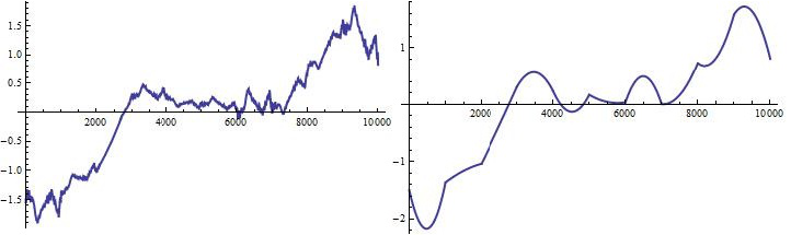
Example 5

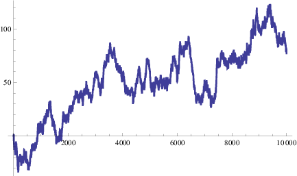
Picture shows Random Walking Graph. It represented by the formula v0=0,vi=vi−1+ξiv_{0}=0,\,v_{i}=v_{i-1}+\xi_{i}, where ξi\xi_{i} is a random value with normal distribution.

Refer to caption
Figure 8: Normalized Random Walking graph.

Interpolation points are x0=0x_{0}=0, x1=1500x_{1}=1500, x2=2000x_{2}=2000, x3=3000x_{3}=3000, x4=4000x_{4}=4000, x5=5500x_{5}=5500, x6=6300x_{6}=6300, x7=7600x_{7}=7600, x8=8000x_{8}=8000, x9=9000x_{9}=9000, x10=10000x_{10}=10000. Applying (7) we obtain d1=−0.237d_{1}=-0.237, d2=0.14d_{2}=0.14, d3=−0.020d_{3}=-0.020, d4=−0.105d_{4}=-0.105, d5=0.105d_{5}=0.105, d6=0.0545d_{6}=0.0545, d7=−0.184d_{7}=-0.184, d8=−0.368d_{8}=-0.368, d9=0.081d_{9}=0.081, d10=−0.111d_{10}=-0.111. Figure 9 shows the graphs of fractal and quadratic approximating functions.

Refer to caption
Figure 9: Fractal and quadratic interpolations of the Random Walking graph.

To compare the results we calculate approximation errors for each type of data. Let h⁡(x)h(x) be the approximating function for data {wm}m=1M\{w_{m}\}_{m=1}^{M}. Then approximation error is

∑m=1MOPEN(h⁡(xm)−wm))2M.\sqrt{\sum\limits_{m=1}^{M}\frac{(h(x_{m})-w_{m}))^{2}}{M}}.

Here we represent the table of approximation errors for each type

F​r​a​c​t​a​lQ​u​a​d​r​a​t​i​cP​o​l​y​n​o​m​i​a​l​F​u​n​c​t​i​o​n0.03590370.0245094D​N​A​P​r​i​m​a​r​y​S​e​q​u​e​n​c​e0.06920720.0624714P​r​i​c​e​G​r​a​p​h0.05013450.0533686R​a​n​d​o​m​W​a​l​k​i​n​g0.10153390.101438\begin{array}[]{ccc}&Fractal&Quadratic\\ PolynomialFunction&0.0359037&0.0245094\\ DNA\,Primary\,Sequence&0.0692072&0.0624714\\ Price\,Graph&0.0501345&0.0533686\\ Random\,Walking&0.1015339&0.101438\end{array}

From it we see, that fractal approximation is better for price graph and nearly equal for random walking, but much worse for smooth function and slightly for DNA sequence. Different results were appearing during calculations of errors. We assume that some conditions could give us more exact approximation results from fractal interpolation function and for that extra observations should be established.

References

  • [1] C. Bandt, A. Kravchenko. Differentiability of fractal curves. Nonlinearity, 24(10):2717–2728, 2011.
  • [2] M. F. Barnsley. Fractals Everywhere. Academic Press Inc., MA, 1988.
  • [3] M. F. Barnsley and L. P. Hurd. Fractal Image Compression. Wellesley, MA:AK Peters, 1993.
  • [4] Feng-lan Bai, Ying-zhao Liu, Tian-ming Wang. A representation of DNA primary sequences by random walk. Mathematical Biosciences 209 (2007) 282–291.
  • [5] J. Hutchinson. Fractals and self similarity. Indiana Univ. Math. J., 30:713–747, 1981.
  • [6] P. Massopust. Interpolation and approximation with splines and fractals. Oxford University Press, Oxford, 2010.
  • [7] H. E. Stanley, S. V. Buldyrev, A. L. Goldbergerb, J. M. Hausdorff, S. Havlin, J. Mietusb, C. K. Peng, F. Sciortino and M. Simons. Fractal landscapes in biological systems: Long-range correlations in DNA and interbeat heart intervals. Physica A 191 (1992) 1–12 North-Holland