A Possible Higher Order Correction to the Chiral Vortical Conductivity in a Gauge Field Plasma
Abstract
The two loop contributions to the chiral vortical conductivity are considered. The Kubo formula together with the anomalous Ward identity of the axial vector current suggest that there may be a nonzero correction to the coefficient of the term of the conductivity.
pacs
12.38.Aw, 24.85.+p, 26.60.+cThe chiral magnetic effect and the chiral vortical effect have been actively investigated for recent years. Because of the triangle anomaly, an external magnetic field and/or an fluid vorticity will induce an electric current, a baryon current and an axial vector current in a relativistic plasma. These currents will lead to separations of electric charges, the baryon numbers and chirality, which may be observed in the quark-gluon plasma created through heavy ion collisions [1, 2]. To the order of the linear response, we have
| (1) |
for the currents driven by the magnetic field and the fluid vorticity. The anomalous transport coefficients ’s above have been exploreded from field theoretic point of view and from the holographic method [1, 3, 4, 5, 6, 7, 8, 9, 10]. An important question along the former approach is if these coefficients are free from the higher order corrections of coupling constants, like their origin, the triangle anomaly. In case of the Chiral Magnetic Effect(CME), the nonrenormalization of in the homogeneous limit of a static magnetic field has been established [11, 12, 13] and the classical expression [1]
| (2) |
holds to all orders of electromagnetic and gauge coupling, where is the number of colors, is the charge number of each flavor and is the chemical potential of the axial charge. The same conclusion for CME can also be reached following the argument in [14]. In this note, we shall address the parallel issue for the chiral vortical conductivity to see whether it is subject to higher order corrections.
The anomalous transport coefficient was first introduced in [7] where the anomalous Ward identity together with the 2nd law of thermodynamics yields for a relativistic plasma with an axial charge chemical potential yields the expression [15]
| (3) |
It is realized soon after in [17] that the general solution to the thermodynamic condition employed in [7] is given by
| (4) |
with a undetermined constant. Then came the Kubo formula [16] and the one-loop calculation in [18] which confirms the general structure (4) and yields . This result is also confirmed by kinetic theories [19]. The authors of [18, 20, 21] related the term to the gravity anomaly and a recent analysis [22] from a geometric point of view within a general hydrodynamical framework suggests the nonrenormalization of the term. But a field theoretic aspect regarding the higher corrections remains murky.
In a recent work [14], the authors addressed the issue based on diagrammatic analysis. They generalized the Coleman-Hill theorem [23] to the stress tensor insertion and proved the nonrenormalization of for a model. As to gauge theories, they argued that the nonrenormalization remains valid in the large limit because of the structure of the anomaly. Upon a close examination of their argument for a gauge theory plasma at the two-loop level, we found a diagram that is not covered. We shall point out this diagram and compute its contribution to below.
For the sake of clarity, we shall consider a QED plasma with the Lagrangian density
| (5) |
where is the electromagnetic field tensor with in gauge potential, the covariant derivative
| (6) |
and we have added couplings to an external axial vector field and a metric perturbation . with the axial vector current
| (7) |
and the stress tensor
| (8) | |||||
We have set in the expression of above. The anomalous Ward identity of reads
| (9) |
with the determinant of the metric .
Following [16], the chiral vortical conductivity is given by the correlators between the axial current density and energy flux density as in the limit , where
| (10) |
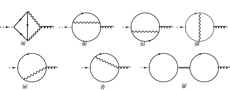
and can be evaluated perturbatively in terms of thermal diagrams, where the Hamiltonian corresponding to the Lagrangian density (5) at . All two-loop diagrams are shown in Fig.1. The one-particle reducible diagram (g) does not contribute since the loop attached to the axial vector vertex vanishes, as can be checked explictly. We have the two-loop contribution to
| (11) |
with
| (12) |
with , and
| (13) |
where with is the Matsubara energy and the photon propagators , and are given by
| (14) |
with and the gauge parameter. The momenta in (11) are all Euclidean with the metric . The amplitudes and of (12) and (13) are related to the anomalous triangle diagram , and the kernel of its metric perturbation , depicted in Fig.2, via
| (15) |
If there were no axial anomaly, the sum of all diagrams (a)-(f) would be of the order in the limit according to the Coleman-Hill like argument employed in [14]. As to the contribution from the anomaly, following an elegant argument of [14], sum of that from Fig. 2(b-f) couples only to the trace of the metric perturbation. Therefore the anomaly does not contribute the diagrams Fig.1(b)-(f) with the insertion of an off-diagonal component. The anomaly contribution to diagram Fig.1(a), however, is not covered by the above argument and has to be examined separately.
The anomalous Ward identity (9) implies that
| (16) |
Taking the derivative with respect to momentum on both sides, we derive
| (17) |
In the absence of infrared divergence, we end up with a nonzero limit as ,
| (18) |
Inserting this nonzero limit into (12), we find the anomaly contribution
| (19) |
Dropping the terms beyond linear order in , we obtain that
| (20) | |||||
with the two-loop contribution to CVE coefficient given by
| (21) |
In the last step, we have dropped the 2nd term in the numerator of the integrand because it is odd in , and have replaced by . The integral of (21) can be calculated by dimensional regularization. We have with
| (22) | |||||
where is the solid angle in dimensions. Therefore
| (23) |
and the coefficient of (4) takes the form
| (24) |
Because of the universality of the axial anomaly, the second term above are intact if the fermion number and the axial charge chemical potentials are switched on. In another word, the of (4) is not renormalized by higher order terms and our result is not in contradiction with the thermodynamic argument of [7].
To convince ourselves the robustness of this result, we have also evaluated a la Pauli-Villars like regularization, which amounts to with
| (25) | |||||
where the coefficients are chosen to make the integral and the summation divergence free. On writing
| (26) | |||||
we have for the first term inside the bracket
| (27) |
with because of the 4d rotational symmetry once the integral is made convergence by the regulators. As to the rest terms, following the standard treatment of the summation over in terms of a contour integral, we find
| (28) |
and confirm (23).

Our analysis can be trivially generalized a QCD like nonAbelian gauge theory with colors and flavors. This amounts to replace of (18) by with the generator for quarks in the fundamental representation and the Yang-Mills coupling and to sum (19) over adjoint gluons. On writing
| (29) |
we have
| (30) |
and the 2nd term is not suppressed in the large limit for a fixed ’t Hooft coupling . This makes the strong ’t Hooft coupling limit nontrivial, an issue that may be addressed by the holographic principle.
One possible loophole with above analysis concerns the generalization of the Coleman-Hill theorem to the stress tensor insertion. In case of the vector or axial current insertion to a diagram with only external gauge boson lines, the transversality of the diagram post insertion can be established algebraically prior to integrating the loop momenta [24] (formally for the axial current case). We find this is not obvious with the stress tensor insertion corresponding to one-loop diagrams with one boson line of each diagram of Fig.1 cut open. The reason may be attributed to the fact that the external lines of the these diagrams do not carry the conserved charges but energies and momenta. If there is no complication with the generalization of the Coleman-Hill theorem, we do find a two loop term of the chiral vortical coefficient given by (23). In any case, it would be interesting to verify or disprove this result through an explicit calculation of all two loop diagrams of Fig.1. Alternatively, the Matsubara formulation of the correlator in (10) can also be evaluated nonperturbatively on a lattice at without running into sign problems.
Acknowledgements.
We are grateful to S. Golkar for email communications on their paper [14] and valuable comments. We are also indebted to him for informing us that they reached a similar conclusion in their forthcoming version of [14] when this work is finished. D. Hou would like to thank S. Lin for valuable discussions. An email communication from K. Landsteiner is warmly acknowledged. This work is supported partly by NSFC under grant Nos. 10975060, 11135011, 11221504 and 10947002.References
- [1] K. Fukushima, D. E. Khareev and H. J. Warringa, The Chiral Magnetic Effect, Phys. Rev. D78, 074033 (2008), arXiv:0808.3382.
- [2] D. E. Khareev and D. T. Son, Testing the Chiral Magnetic Effect and Chiral Vortical Effects in Heavy Ion Collisions, Phys. Rev. Lett. 106, 062301 (2011), arXiv:1010.0038.
- [3] H. U. Yee, Holographic Chiral Magnetic Conductivity, JHEP 0911, 085 (2009), arXiv:0908.4189.
- [4] J. Erdmenger, M. Haack, M. Kaminski and A. Yarom, Fluid Dynamics of R-charged Black Holes, JHEP 0901, 055 (2009), arXiv:0809.2488.
- [5] N. Banerjee, J. Bhattacharya, S. Bhattacharyya, S. Dutta, R. Loganayagam and P. Surowka, Hydrodynamics from Charges Black Branes, JHEP 1101, 094 (2011), arXiv:0809.2596.
- [6] M. Torabian and H. U. Yee, Holographic Nonlinear Hydrodynamics from AdS/CFT with Multiple/non-Abelian Symmetries JHEP 0908, 020 (2009), arXiv:0903.4894.
- [7] D. T. Son and P. Surowka, Hydrodynamics with Triangle Anomalies, Phys. Rev. Lett., 103, 191601 (2009), arXiv:0906.5044.
- [8] T. Kalaydzhyan and I Kirsch, Fluid/gravity Model for the Chiral Magnetic Effect, Phys. Rev. Lett. 106, 211601 (2011), arXiv:1102.4334.
- [9] Shu Lin, An Anomalous Hydrodynamics for Chiral Superfluid, arXiv:1112.3215.
- [10] V. P. Nair, R. Ray and S. Roy, Fluids, Anomalies and the Chiral Magnetic Effect: A Group-theoretic Formulation, arXiv:1201.6609.
- [11] V. Rubakov, On Chiral Magnetic Effect and Holography, arXiv:1005.1888.
- [12] D. K. Hong, Anomalous Currents in Dense Matter under a Magentic Field, Phys. Lett. B699, 305 (2011), arXiv:1010.3923.
- [13] Defu Hou, Hui Liu and Hai-cang Ren, Some Field Theoretic Issues Regarding the Chiral Magnetic Effect, JHEP 1105, 046 (2011), arXiv:1103.2035.
- [14] S. Golkar and D. T. Son, Non-Renormalization of the Chiral Vortical Effect Coefficient, arXiv:1207.5806.
- [15] The vertical conductivity in [7] is defined in Landau frame, given by with , and the axial-charge density, the energy density and the pressure of the fluid. The 2nd term inside the parentheses represents the contribution from the energy flow and is subtracted out in this paper. See [16] for clarifications.
- [16] I. Amado, K. Landsteiner and F. Pena-Benitez, Anomalous Transport Coefficients from Kubo formulas and Holography, JHEP 1105 081 (2011).
- [17] Y. Neiman and Y. Oz, Relativistic Hydrodynamics with General Anomalous Charges, JHEP 1103, 023 (2011), arXiv:1011.5107.
- [18] K. Landsteiner, E. Megias and F. Pena-Benitez, Gravitational Anomaly and Transport, Phys. Rev. Lett., 107, 021601 (2011), arXiv:1103.5006.
- [19] J. H. Gao, Z. T. Liang, S. Pu, Q. Wang and X. N. Wang, Chiral Anomaly and Local Polarization Effect from Quantum Kinetic Approach, arXiv:1203.0725.
- [20] K. Landsteiner, E. Megias, L. Melgar and F. Pena-Benitez, Holographic Gravitational Anomaly and Chiral Vortical Effect, JHEP 1109, 121 (2011), arXiv:1107.0368.
- [21] S. Chapman, Y. Neiman and Y. Oz, Fluid/gravity Correspondence, Local Wald Entropy and Gravitational Anomaly, JHEP 1207, 128 (2012), arXiv:1202.2469.
- [22] K. Jensen, R. Loganayagam and A. Yarom, Thermodynamics, Gravitational Anomalies and Cones, arXiv:1207.5824.
- [23] S. Coleman and B. Hill, No More Corrections to Topological Mass Term in QED3, Phys. Lett. 159B, 184 (1985).
- [24] J. Bjorken and S. Drell, Relativistic Quantum Fields, McGraw-Hill Book Company, 1965, Sect. 17.9.