Analytical study of spin-dependent transition rates within pairs of dipolar and strongly exchange coupled spins with ($S=1/2$) during magnetic resonant excitation

In recent years, various experimental [1, 2, 3, 4, 5] studies focusing on the nature of spin–dependent charge carrier transport and recombination processes have been conducted by using a coherent magnetic resonant spin manipulation. The idea of these pulsed electrically and optically detected magnetic resonance experiments (pEDMR, pODMR, respectively) is to identify an induced coherent spin propagation by observables that are directly controlled by coherent spin motion. Typically, for pEDMR and pODMR, a powerful oscillating driving field is applied in magnetic resonance to the explored spin system, and the resulting Rabi oscillation is then observed electrically or optically. From the Rabi oscillation components, information about the Hamiltonian of the propagating system and, therefore, about its physical nature can be obtained. While this experimental approach is similar to the way coherent spin motion is observed with conventional pulsed electron paramagnetic resonance (pEPR), the different observables prohibit a direct comparison of pEPR and pEDMR/pODMR experiments. This difference of observables has been subject of a number of theoretical studies[6, 7, 8, 9, 10] in recent years. Most experimental and theoretical studies have focused on spin–selection rules induced by the Pauli blockade. Pauli blockade exists when a transition between two localized paramagnetic, singly occupied electron states into one doubly occupied singlet states is controlled by the pair state of the two $S=1/2$ spins before the transition. This so called intermediate pair model was first described by Kaplan, Solomon and Mott[11] in 1978. Based thereon, successful descriptions of spin–dependent processes observed with EDMR and ODMR and in particular for pEDMR and pODMR experiments have been possible. Most of these theoretical studies used numerical methods in order to scrutinize experimental insights. This approach however does not allow the derivation of analytical expressions needed for the fit of experimental data and which can also limit fundamental qualitative understanding. Only recently, first analytical descriptions of coherently controlled spin–dependent intermediate pair transitions rates have been derived in Ref. 10, this work however applies only to intermediate pairs with negligible exchange and spin–dipolar interaction.

When intermediate spin $S=1/2$ pairs, consisting of two pair partners $a$ and $b$, are weakly coupled, then the Rabi oscillations in each partner take place independently as illustrated in Fig. 1a. The spin–Rabi oscillation frequencies of the pair partners will then become

where $\Omega_{\scriptscriptstyle R}=\gamma B_{\scriptscriptstyle 1}$ is the Rabi nutation frequency, $B_{\scriptscriptstyle 1}$ is the magnitude of the driving ac magnetic field, and $\gamma$ is gyromagnetic ratio; $\delta_{\scriptscriptstyle a}=\omega_{\scriptscriptstyle a}-\omega$, and $\delta_{\scriptscriptstyle b}=\omega_{\scriptscriptstyle b}-\omega$ are the differences (the so called detuning) of the pair partners Larmor frequencies $\omega_{\scriptscriptstyle a}$ and $\omega_{\scriptscriptstyle b}$ from the excitation frequency $\omega$ (see Fig. 1a). For independent oscillations, the Rabi spectrum, ${\bf\mathrm{F}}(s)$, of electrically detected magnetic resonance will contain the lines

The lines $s_{\scriptscriptstyle 1}^{\scriptscriptstyle a}$ and $s_{\scriptscriptstyle 1}^{\scriptscriptstyle b}$ correspond to precession of one of the two pair partners, whereas the $s_{\scriptscriptstyle 2}$-line[6, 4, 7] (and also the $s_{\scriptscriptstyle 0}$-line[10] ) originates from coherent precession of both pair partners around $B_{\scriptscriptstyle 1}$ in the rotating frame, they are beat Rabi–beat components due to the relative spin motion of the two pair partners.

In the present paper we address the question of how the process in Fig. 1a gets modified when the pair partners are coupled by strong exchange $J\gg\Omega_{\scriptscriptstyle R},\delta_{\scriptscriptstyle a},\delta_{\scriptscriptstyle b}$ and non–negligible spin–dipolar interaction. We demonstrate that, in the limit of strong exchange, the Rabi oscillations are intrinsically collective and proceed according to the following scheme

Fig. 1b shows an illustration of this scheme which does not involve the singlet state, $\frac{1}{\sqrt{2}}(\downarrow\uparrow-\uparrow\downarrow)$, which, as we demonstrate below, gets decoupled in the domain $J\gg\Omega_{\scriptscriptstyle R},\delta_{\scriptscriptstyle a},\delta_{\scriptscriptstyle b}$.

We will show that, in the limit of large $J$, the spectrum of the Rabi oscillations is governed by the interplay of the Rabi frequency, $\Omega_{\scriptscriptstyle R}$, dipole-dipole interaction magnitude, $D$, and the average detuning, $\delta$. As anticipated for a two $S=1/2$ system which gradually turns into one $s=1$ system with increasing $J$, the magnitude, $J$, of the exchange coupling drops out from the theory and the spectrum is governed by a single dimensionless combination of parameters, $\Omega_{\scriptscriptstyle R}$, $D$, and $\delta$. From previous numerical studies of exchange coupled intermediate pairs [8] it is known that due to the change of the two $S=1/2$ system into one $S=1$ system, EDMR and ODMR induced rate changes becomes negligibly small. Qualitatively, this can be understood by the realization that in presence of large $J$, magnetic resonance will always change triplet states into triplet states and the singlet to triplet ratio is therefore not changed. However, the results presented here can still be of significance as long as $J$ is large but not many orders of magnitude larger than dipolar or the Rabi nutation frequency.

Our main finding is that, upon the change of this parameter, the spectrum, ${\bf\mathrm{F}}(s)$, exhibits a non-trivial evolution. Peculiarity of ${\bf\mathrm{F}}(s)$ manifests itself in the behavior of the Rabi spectral lines at small $\Omega_{\scriptscriptstyle R}\lesssim D$. For two-level systems, the frequencies of oscillations always grow with increasing $\Omega_{\scriptscriptstyle R}$. We find that, for the dipole-dipole coupled system in Fig. 1b, the Rabi spectrum contains three frequencies one of which decreases with $\Omega_{\scriptscriptstyle R}$. Upon subsequent increase of $\Omega_{\scriptscriptstyle R}$, this frequency passes through a minimum and grows as $s\approx\Omega_{\scriptscriptstyle R}$ at large $\Omega_{\scriptscriptstyle R}\gg D$. In addition, we find that the behavior of this spectral line with detuning, $\delta$, also exhibits a minimum. Moreover, we find that a minimum in the position of the Rabi spectral line is accompanied by a maximum in its intensity. The definition of the line intensity pertinent to electrically detected magnetic-resonance experiments [1, 2, 3, 4, 5, 12, 13, 14, 15] is given below. Finally, we demonstrate that the disorder with r.m.s., $\Delta$, in Larmor frequencies of the pair partners leads to a Gaussian broadening of the Rabi spectral lines, and express the corresponding widths in terms of $\Delta$, $\Omega_{\scriptscriptstyle R}$, $D$, and $\delta$.

In the previous numerical studies of the of the Rabi oscillation Fourier spectra[7, 8, 9], the frequencies of oscillations were found for various sets of parameters and different relations between $J$, $\Omega_{\scriptscriptstyle R}$, $\delta_{\scriptscriptstyle a}$ and $\delta_{\scriptscriptstyle b}$. Here, we restrict our consideration to the domain of large $J$, but within this domain our treatment is fully analytical.

The paper is organized as follows: In Sect. II we relate the time-dependent populations of different spin states involved in the Rabi oscillations of pairs to the observable quantity, namely, photoconductivity measured during pEDMR experiments. In Sect. III we analyze the quasienergies of a resonantly driven spin pair in the limit of strong exchange. In Sect. IV general expressions for positions and intensities of the Rabi spectral lines are derived. These expressions are analyzed in Sect. IV. In Sect. V we discuss the relation of spin-Rabi oscillations in a coupled pair to the excitonic Rabi oscillations in quantum dot molecules.

For pEDMR experiments, a samples’ conductivity change, $\Delta\sigma$, is measured upon application of a short resonant magnetic resonant pulse [6]. More specifically, the dynamics, $\Delta\sigma(t)$, of the return of conductivity to the steady state after the pulse ends is measured as a function of the pulse duration, $\tau$. This duration is much shorter than all intrinsic times, so that the change of conductivity during the interval, $\tau$, is negligible. Dependence of $\Delta\sigma(t)$ on $\tau$ originates from the fact that the pulse rotates the spins of the pair partners. On the other hand, the spin state of the pair serves as initial condition for the process of the conductivity recovery. In this way, PEDMR measurements provide information about the Rabi oscillations within the pair of spins.

A very important observation made in Ref. 6 is that the contribution to photoconductivity, $\Delta\sigma$, comes from specific spin configurations both in initial and in final states. More specifically, when thermal polarization is negligibly small and the system is in a steady state, the initial state of the pair at the moment, $t=0$, of application of the microwave pulse is either $\downarrow\downarrow$, or $\uparrow\uparrow$, with equal probability. If the system was initially in $\downarrow\downarrow$, the contribution to $\Delta\sigma$ is proportional to $|A^{\scriptscriptstyle\downarrow\downarrow}_{\scriptscriptstyle\downarrow\downarrow}(\tau)|^{2}+|A^{\scriptscriptstyle\downarrow\downarrow}_{\scriptscriptstyle\uparrow\uparrow}(\tau)|^{2}$, where $A_{\scriptscriptstyle\downarrow\downarrow}^{\scriptscriptstyle\downarrow\downarrow}(\tau)$ and $A_{\scriptscriptstyle\uparrow\uparrow}^{\scriptscriptstyle\downarrow\downarrow}(\tau)$ are the amplitudes to find the system, respectively, in $\downarrow\downarrow$ and $\uparrow\uparrow$ at time $\tau$, which is the duration of the pulse. The upper indices indicate that the amplitudes are calculated with initial condition that at $t=0$ the system is in $\downarrow\downarrow$. Correspondingly, if at $t=0$ the system was in $\uparrow\uparrow$, the contribution to $\Delta\sigma$ is proportional to $|A^{\scriptscriptstyle\uparrow\uparrow}_{\scriptscriptstyle\downarrow\downarrow}(\tau)|^{2}+|A^{\scriptscriptstyle\uparrow\uparrow}_{\scriptscriptstyle\uparrow\uparrow}(\tau)|^{2}$. Therefore, the quantity, $\Delta\sigma$, measured by PEDMR techniques should be identified with the following combination of quantum-mechanical probabilities

Each of the probabilities contains three oscillating components of the form $\cos s\tau$. Thus, the Fourier analysis of measured $\Delta\sigma(\tau)$ should reveal three peaks. We define the intensity of the Rabi spectral line as a magnitude of the corresponding oscillating component in the sum Eq. (4).

We start from the Hamiltonian of the pair

where the first three terms represent the Hamiltonian of the ac driven pair partners and the last two terms describe the intra-pair exchange and dipole-dipole interactions.

To study the time evolution of the spin-pair one has to solve the Schrödinger equation, $i\frac{\partial}{\partial t}\Psi(t)=\hat{H}\Psi(t)$, for the four-component wave function

of the amplitudes of different spins states. These amplitudes satisfy the following system of equations

where the asymmetry parameter, $\delta_{\scriptscriptstyle 0}$ is defined as

The quasienergies, $\chi$, of the system of equations Eq. (7) are introduced in a standard way, by using the following substitutions

and employing the rotating-wave approximation. Then the system Eq. (7) reduces to the following system of algebraic equations

where we introduced the detuning parameter

The system Eq. (10) can be reduced to two coupled equations for the amplitudes $a_{\scriptscriptstyle\uparrow\downarrow}$ and $a_{\scriptscriptstyle\downarrow\uparrow}$, which read

where $\tilde{\chi}=\chi+\frac{1}{2}(J+D)$. Multiplying Eqs. (12) and (13) gives the following quartic equation for the quasienergies

The form Eq. (14) of the characteristic equation explains on the quantitative level the statement made in the Introduction that, at large $J$, the magnitude of exchange drops out from the theory. Indeed, if the asymmetry parameter $\delta_{\scriptscriptstyle 0}$ is much smaller than $(JD)^{1/2}$, $(J\Omega_{\scriptscriptstyle R})^{1/2}$, the last terms in the brackets, containing $J$ in the denominator, can be neglected. More precisely, under the condition $\delta_{\scriptscriptstyle 0}\ll(JD)^{1/2},(J\Omega_{\scriptscriptstyle R})^{1/2}$, the quasienergy $\tilde{\chi}\approx J+\frac{D}{2}$, corresponding to the singlet, is much bigger than three other quasienergies. As a result, only three triplet states $A_{\scriptscriptstyle\uparrow\uparrow}$, $A_{\scriptscriptstyle\downarrow\downarrow}$, and $\frac{1}{\sqrt{2}}(A_{\scriptscriptstyle\uparrow\downarrow}+A_{\scriptscriptstyle\downarrow\uparrow})$ participate in the Rabi oscillations. On the qualitative level, decoupling of the singlet state, $\frac{1}{\sqrt{2}}(A_{\scriptscriptstyle\uparrow\downarrow}-A_{\scriptscriptstyle\downarrow\uparrow})$, originates from the fact that exchange does not mix this state with components of the triplet.

In the limit of strong exchange Eq. (14) reduces to a cubic equation

Obviously, for $D\ll\Omega_{\scriptscriptstyle R}$, $\delta$, we recover the conventional Rabi oscillations

In the opposite limit, when $D\gg\Omega_{\scriptscriptstyle R},\,\delta$, we have

so the difference $\chi_{\scriptscriptstyle 2}-\chi_{\scriptscriptstyle 3}$, which is the position of the lowest spectral line, behaves as $s=\frac{2}{3D}\Omega_{\scriptscriptstyle R}^{2}$. The positions of other two lines are close to $s=\frac{3}{2}D$.

To assess the intermediate regime, $\delta\sim D$, we rewrite the cubic equation, Eq. (15), by using the dimensionless variable,

where

Then it assumes the form

We see that quasienergies, ${\tilde{\chi}}_{\scriptscriptstyle i}$, are determined by a single dimensionless combination of parameters $\Omega_{\scriptscriptstyle R}$, $D$, and $\delta$, defined as

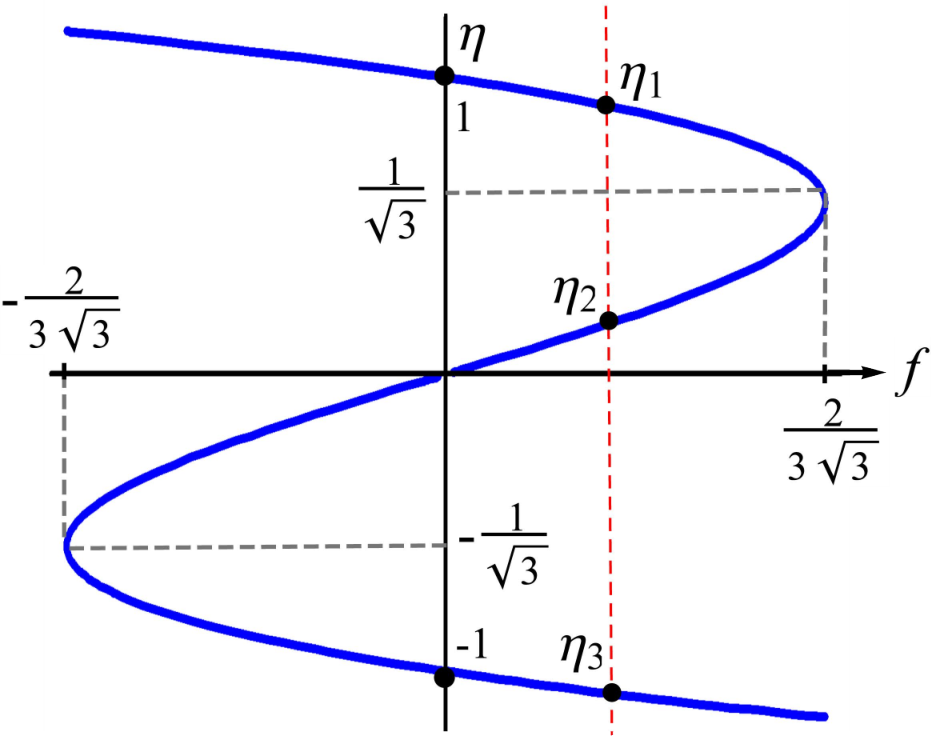
It is easy to check that for any $D,\,\delta,$ and $\Omega_{\scriptscriptstyle R}$ the parameter $f$ resides within the interval $-\frac{2}{3\sqrt{3}},\frac{2}{3\sqrt{3}}$, which ensures that all three roots, $\eta_{\scriptscriptstyle i}$, are real. Graphic solution of Eq. (20) is illustrated in Fig. 2. Analytic expressions for the roots, $\eta_{\scriptscriptstyle i}$, are the following

where the phase $\psi$ is determined as

To find the quasienergies, ${\tilde{\chi}}_{\scriptscriptstyle i}$ for given values of $D$, $\delta$, and $\Omega_{\scriptscriptstyle R}$, one has to calculate parameter $f$ from Eq. (21), substitute it into Eq. (22) for $\eta_{i}$, and, finally, substitute $\eta_{i}$ into Eq. (18). The evolution of ${\tilde{\chi}}_{\scriptscriptstyle i}$ with $\Omega_{\scriptscriptstyle R}$ and $\delta$ is governed by the dependence of $f$ on these parameters, which can be tuned externally. Fig. 3 illustrates that this evolution is quite nontrivial, namely, $f$ exhibits extrema both as function of $\Omega_{\scriptscriptstyle R}$ and as a function of $\delta$.

The eigenvectors of the system Eq. (10) corresponding to the roots can be conveniently cast in the form

We are now in position to calculate the population of the state $\frac{1}{\sqrt{2}}(A_{\scriptscriptstyle\uparrow\downarrow}+A_{\scriptscriptstyle\downarrow\uparrow})$ as a function of time. The general expression for $|A_{\scriptscriptstyle\uparrow\downarrow}+A_{\scriptscriptstyle\downarrow\uparrow}|^{2}$ can be written as

where the three constants $C_{1}$, $C_{2}$, and $C_{3}$, are determined from three initial conditions. Assuming that at $t=0$ the pair of spins is in $\downarrow\downarrow$ state, so that $A_{\scriptscriptstyle\downarrow\downarrow}(0)=1$, $A_{\scriptscriptstyle\uparrow\uparrow}(0)=0$, $(A_{\scriptscriptstyle\uparrow\downarrow}(0)+A_{\scriptscriptstyle\downarrow\uparrow}(0))=0$, and solving the system of three linear equations we find

At this point we note that the population Eq. (25) is directly related to the photoconductivity, $\Delta\sigma$, Eq. (4). Indeed, $1-|A_{\scriptscriptstyle\uparrow\downarrow}+A_{\scriptscriptstyle\downarrow\uparrow}|^{2}$ is a probability to find the system either in $\downarrow\downarrow$ state or in $\uparrow\uparrow$ state after the time $t$.

The second contribution to $\Delta\sigma$ comes from realizations in which the system is initially in the $\uparrow\uparrow$ state. It is easy to see that this contribution can be obtained by simply changing $\delta$ by $-\delta$ in Eq. (26). In terms of the Fourier transform, as it follows from Eqs. (4) and (25), $\Delta\sigma$ will contain the three peaks: upper, lower, and middle, with positions

and corresponding intensities

In the next Section we analyze how the peak positions and magnitudes evolve with $\Omega_{\scriptscriptstyle R}$.

In the previous section we derived analytical expressions for the positions of the Rabi spectral lines and their intensities, see Eqs. (27) and (28). Below we analyze the evolution of the spectrum with increasing the amplitude, $\Omega_{\scriptscriptstyle R}$, of the driving ac field and with detuning, $\delta$.

We have derived an analytical description of spin–dependent electronic transition rates within strongly exchange coupled intermediate pairs during a coherent spin excitation which revealed the influence of several spin–Rabi oscillation components whose intensities and frequencies depend on the dipolar coupling within the pair, the strength of the driving field as well as the detuning. As long as the exchange coupling is strong, the oscillations controlling spin–dependent rates do neither depend of the value of the exchange coupling nor on the spin–orbit or hyperfine field induced Larmor separation (the difference of the pair partners Larmor frequencies). It must be emphasized that “strong exchange” in the context of this work means that $J$ is larger than all other relevant parameters (dipolar strength, Larmor separation, driving field strength, and detuning) but not many orders of magnitude stronger. While the conclusions of the work presented here remain unchanged by the magnitude of $J$, very large $J$ will lead to rapidly decaying rate changes which will render the results irrelevant for their experimental application.

Obtaining the solutions analytically has been possible because in the limit of strong exchange, only three out of four spin states of the pair participate in the Rabi oscillations. Note that there exists another prominent object in which Rabi oscillations take place within a system of three levels. This object is a quantum dot molecule[17, 18, 19, 20, 21, 22, 23], in which the excitation energy lies in the optical range. The analog of spin is played by a two-level system consisting of size-quantized electron and hole levels in a self-assembled quantum dot. Experimentally, Rabi oscillations between these two levels are studied by optical[24, 25], and electrical[26] techniques. The quantum dot molecule represents two vertically aligned quantum dots, so that electron excited in one dot can tunnel into another dot and vice versa. This tunneling is a source of coupling between the dots which has no analog in spin pair considered in the present paper. The other mechanism by which different dots “communicate” with each other is the Coulomb attraction of excited electron to the hole left behind. If hole resides in one dot, the energy of attraction of electron to this hole is different depending whether electron resides in the same dot or in the neighboring dot. This difference mimics the dipole-dipole interaction in the spin system we considered. The most important difference between the two systems lies in the structure of three levels participating in the Rabi oscillations. In the spin pair these levels are shown in Fig. 1b and are almost evenly spaced in energy. In quantum dot molecules the relevant levels are: the ground state with no exciton, excited state with one exciton in the left dot, and excited state with one exciton in the right dot, so that two excited states are close in energy.

As a final remark, note that Rabi oscillations in quantum dot molecules recently reported in Ref. 27 correspond to simultaneous Rabi nutations of two electrons. This is similar to the Rabi oscillations under the conditions of half-field magnetic resonance which were also recently observed experimentally[15].