The Quantum Adiabatic Algorithm
applied to random optimization problems:
the quantum spin glass perspective
Abstract
Among various algorithms designed to exploit the specific properties of quantum computers with respect to classical ones, the quantum adiabatic algorithm is a versatile proposition to find the minimal value of an arbitrary cost function (ground state energy). Random optimization problems provide a natural testbed to compare its efficiency with that of classical algorithms. These problems correspond to mean field spin glasses that have been extensively studied in the classical case. This paper reviews recent analytical works that extended these studies to incorporate the effect of quantum fluctuations, and presents also some original results in this direction.
Keywords:
Quantum spin glasses , Quantum annealing , Quantum adiabatic algorithm , Computational complexity1 Introduction
A central issue in computer science is the classification of the difficulty of computational tasks, i.e. the existence or not of algorithms with small requirements (in terms of the time of execution and the necessary memory) that perform a given task [1, 2]. This classification is called computational complexity theory. A rough distinction between easy and hard tasks is made by distinguishing algorithms that need to perform a number of elementary operations growing either polynomially or exponentially with the size of their input. One of the central tasks analyzed in this context concerns combinatorial optimization problems [3]: given a cost function defined on variables, each taking a finite number of values, the question is to classify families of cost functions such that algorithms can, or cannot, find their global minimum by executing a number of operations smaller than some polynomial of . The current consensus is that there exist families of cost functions such that no algorithm can achieve this goal (this is the famous PNP conjecture). One example of such difficult problems is the graph -coloring (for ): given a graph, i.e. a collection of vertices and edges linking some of the pairs of vertices, the cost function associates to each of its -coloring (one out of colors is chosen for each vertex) the number of monochromatic edges, linking two vertices of the same color.
It was understood above that the term “elementary operation” meant some simple process like adding two numbers, or other arithmetic tasks, which can all be reduced to logical operations on boolean variables. In that context the basic elements of a computer are bits that behave “classically”, i.e. they are in a well defined state 0 or 1, that is altered deterministically by logical operations involving one or a few of them. But what happens if the basic elements of a computer behave “quantumly”, i.e. if instead of bits one deals with “qubits” that can not only be in the states 0 or 1 but in any linear combination of the two? Will such a quantum computer be able to solve efficiently some of the tasks on which classical computers get stuck? These questions were first raised in the eighties by Feynman [4] and Deutsch [5] and opened the way to a new branch of science at the interface between computer science and physics, known today under the names of quantum computing and quantum information theory [6, 7, 8].
Several specific quantum algorithms have been discovered since then [5, 9, 10, 11, 12], providing “quantum speedup” with respect to their fastest classical counterparts. Most of them concern arithmetic problems, notably Shor’s algorithm for factoring integers [11], yet none of them solves efficiently a representant of the classically hardest problems (the so-called NP-complete ones). A quantum analog of the computational complexity theory has been developed [13, 14, 15], with the introduction of complexity classes of easy and hard problems, the notion of difficulty being now with respect to the number of required operations on a quantum, instead of classical, computer.
A generic strategy to solve optimization problems with a quantum computer, called quantum annealing or quantum adiabatic algorithm [16, 17, 18, 19, 20], proceeds in the following way (see [21, 22, 23, 24] for reviews of this procedure). The evolution of the state of a quantum computer obeys Schrödinger equation, with a time-evolving Hamiltonian that is controlled by the programmer. If in an initialization step the system is prepared in the ground state of a simple Hamiltonian , and if the time evolution of the Hamiltonian is slow enough, the adiabatic theorem [25] ensures that the system remains, with high probability, in the instantaneous ground state at all subsequent times. This property can be exploited by driving the Hamiltonian towards one that corresponds to the cost function of the optimization problem to be solved, let us call it . Indeed its ground state, which is the final state of the system according to the adiabatic theorem, provides precisely the answer to the combinatorial optimization problem. The crucial question of the efficiency of such an algorithm reduces thus to a criterion for the validity of the adiabatic approximation. Roughly speaking the adiabatic theorem states that the evolution time of the Hamiltonian (hence the running time of the algorithm) has to be larger than the inverse square of the minimal energy gap between the ground state and the first excited state encountered during the process. Instances of optimization problems such that this gap is exponentially small in the size of the problem (and thus require an exponentially large time to be solved adiabatically) were exhibited early on [26, 27]. It was also realized that some choices of the initial Hamiltonian led ineluctably to exponentially small gaps [28, 29].
One can however wonder if, for “reasonable” choices of , and for “most instances” belonging to hard optimization problem classes, this annealing procedure leads to a quantum speedup with respect to classical algorithms. A precise meaning can be given to the expression “most instances” by considering ensemble of random instances. Continuing with the example of the graph coloring problem defined above, one can for instance define probability laws on the set of all graphs of vertices, the most famous one being the Erdős-Rényi random graph [30] in which the edges are chosen uniformly at random. Then a property holds for “most instances” if its probability with respect to the choice of the random graph goes to 1 in the large size (thermodynamic) limit . Such ensembles of random optimization problems were actually introduced in computer science [31] as generators of hard problems on which to benchmark classical algorithms. Since then an intense research effort was devoted to their study, in theoretical computer science and discrete mathematics of course, but also in statistical mechanics. Random optimization problems can indeed be handled by methods first devised for the study of disordered physical systems, spin glasses in particular [32]: renaming energy the cost function, optimization amounts to low temperature statistical mechanics (one can view for instance the graph coloring problem as an antiferromagnetic -states Potts model), an optimal configuration becomes a ground state, and the randomness in the instance corresponds to the quenched disorder of spin glasses. This interdisciplinary approach turned out to be very fruitful, and in the last decade a detailed understanding of the shape of the configuration space of random optimization problems was reached thanks to the non-rigorous methods of statistical mechanics (some of these predictions were later on put on a rigorous mathematical basis). In the thermodynamic limit these problems undergo several phase transitions when some control parameter of the random ensemble (for instance the finite ratio in the case of the graph coloring) is varied, in particular the set of ground states gets split into a large number of clusters of close-by configurations, the clusters being well separated one from the other in the configuration space. This understanding also allowed to devise specific ensembles of random instances where one can “hide” an arbitrarily chosen unique ground state, that remains hard to find if no direct information is available on the hidden configuration. This is particularly useful in the context of the quantum adiabatic algorithm, which has most often been studied on instances with a Unique Satisfying Assignment (USA).
As explained above the random optimization problems provided useful benchmarks for classical algorithms, it is thus natural to test the efficiency of the quantum adiabatic algorithm on them, and indeed one of the first proposals [20] studied such random instances. Unfortunately simulating quantum computers on classical ones is a hard computational task because the dimension of the Hilbert space grows exponentially with the number of qubits, hence the numerical integration of Schrödinger equation, or the exact diagonalization of the time-varying Hamiltonian is restricted to rather small system sizes, whereas computational complexity theory classifies the difficulty of problems in the infinite size limit. However random optimization problems, viewed from the perspective of statistical mechanics of disordered systems, are mean field systems (there is no finite-dimensional lattice underlying their definitions) and are as such amenable to an analytic resolution. It is thus possible to build upon their classical statistical mechanics studies in order to include the quantum effects induced by the interpolation procedure at the core of the quantum annealing procedure. In particular one can investigate the fate of the classical phase transitions mentioned above when quantum effects are added; when these become quantum phase transitions [33] as a function of the time parameter of the adiabatic interpolation, energy gaps close in the thermodynamic limit and this sets a lower bound on the running time of the algorithm, as the adiabatic criterion has to be fulfilled. It is thus of a crucial importance to understand the quantum phase transitions of random constraint satisfaction problems in presence of quantum fluctuations, and in particular their order: generically second order phase transitions are associated to polynomially small gaps, while first order transitions (which are commonly found in quantum mean field spin glasses [34, 35, 36, 37, 38]) cause exponentially small gaps, and in consequence an exponentially long evolution time is required for the adiabatic criterion to hold. Another, distinct, mechanism for the appearance of small gaps was pointed out in [39, 40], based on an analysis of the perturbative effects of quantum fluctuations on the classical energy levels of optimization problems. Some variants of the quantum adiabatic algorithm were claimed to circumvent the effects of these “perturbative crossings” in [41, 42, 43].
In this brief presentation, as in most of the literature, the quantum adiabatic algorithm is viewed as an algorithm to find the ground state of an Hamiltonian, or in computer science terms to solve exactly an optimization problem. One can however think of it more generically as an approximation algorithm [44]: if the allowed evolution time is smaller than required by the adiabaticity criterion then the system ends up in an excited state, corresponding to energies higher than the global minimum of the Hamiltonian (this is, in physical terms, reminiscent of the Kibble-Zurek problem, see [45] for a recent review). But it might be that a good compromise can be found between short execution times on the one hand, and small excitation energies on the other hand. This would be as important from a complexity point of view as being able to find the exact ground state. Indeed for several optimization problems it is computationally hard to find an approximate value of the ground state energy, and for some of them it is hard even to make an estimate better than the energy of a configuration chosen uniformly at random [46].
In this paper we shall review and extend recent works on the behaviour of the quantum adiabatic algorithm on random optimization problems. As we explained above this is strongly related to the understanding of the low temperature phases of quantum spin glasses. The paper is organized as follows. In Sec. 2 we shall make a brief introduction to classical and quantum computational complexity theory, and define more precisely the quantum adiabatic algorithm. Sec. 3 contains a review on classical random optimization problems, their phase transitions and their relations to spin glasses. Special attention will be given in Sec. 3.9 to the problem of generating random instances with prescribed properties, in particular to ensure the non-degeneracy of the ground state (USA instance). In Sec. 4 we discuss the thermodynamic properties of quantum spin glasses, concentrating in particular on their low energy properties and quantum phase transitions, without entering into technical details. The latter are touched upon in Sec. 5, where we present several methods, both analytical and numerical, for the study of quantum disordered systems. Some of these methods are then applied to a few representative examples of random optimization problems subject to quantum fluctuations in Sec. 6. We finally draw our conclusions in Sec. 7.
In addition to its review character this paper contains original material: in Sec. 4.4 and 6.2 we present some details and additional results of two works that previously appeared as letters [47, 48]; among the results of these sections the study of the gap in presence of an exponential degeneracy of the ground state in Sec. 6.2.2 should have a general relevance. The discussion of the quantum -coloring (or antiferromagnetic Potts model) in Sec. 6.3 was not published before and will be further developed in a forthcoming publication [49]. In Sec. 5.6 we propose a method to extract the gap from Quantum Monte Carlo (QMC) numerical simulations, that, to the best of our knowledge, was not discussed previously. The discussion on the generation of USA instances of Sec. 3.9 also bears some originality in the quantum context. Finally, in Sec. 5.6.3 and 6.2.3 we show how one can use QMC simulations to detect the clustering transition (to be introduced in Sec. 3) of quantum models.
2 Classical and quantum computations
2.1 Classical computation theory
2.1.1 Examples of optimization problems
We shall give in this section a brief introduction to the classical theory of computational complexity [1, 3, 2], and set up some notations that we shall use in the rest of the paper. For concreteness we will concentrate on computational tasks related to combinatorial optimization problems. We shall thus consider a discrete configuration space of variables denoted , each of them taking values in a finite set , and denote a global configuration . In most computer science applications the variables considered are boolean, and one usually takes or . For consistency with the conventions in vigor in physics we shall also use , the translations between the various conventions being straightforward. The computational tasks we are interested in are defined in terms of a cost function that assigns to each configuration a real number. We will call this cost the energy of the configuration, or the value of its Hamiltonian, and denote it . Let us give some examples:
- 1.
The graph -coloring problem, in short -COL, was mentioned in the introduction and is formalized as follows. Given a graph with a set of vertices and a set of edges between pairs of vertices, one takes , with an arbitrary integer, so that each configuration corresponds to the coloring where vertex is given the color . The cost function is
(1) where the sum runs over all edges of the graph, and denotes the Kronecker symbol. The cost function thus counts the number of monochromatic edges in the configuration .
The following examples involve binary variables that, as explained above, we encode with Ising spins, .
- 1.
The -XORSAT problem is defined on a -hypergraph : each of the hyper-edges involves a -uplet of variables, with , thus generalizing the notion of usual graphs that corresponds to . We label the hyper-edges with an index , and denote the indices of the vertices linked by the -th hyper-edge. In addition to the hyper-graph the problem is defined by constants , and the cost function reads
(2) It is easily seen that this sum equals the number of hyper-edges for which the condition is violated. There are various equivalent interpretations of this condition; in the language of coding theory [53] this is a parity check rule. By associating Ising spins to variables according to it is also equivalent to a linear equation of the form , where and the additions are interpreted modulo 2. Finally it can be seen as a condition on the eXclusive OR of boolean variables , hence the name of the problem.
- 2.
In the -SAT problem one is given an hypergraph and, for each hyper-edge, constants ; the cost of a configuration is then defined as
(3) Each term of the sum is equal to 1 if, for all the vertices involved in that hyper-edge, one has ; on the contrary it vanishes as soon as one of the vertices fulfill . In terms of boolean variables this is the disjunction (logical OR) of literals, that are equal to a variable or its logical negation depending on the sign of .
- 3.
Another example is the so-called -in- SAT (or Exact Cover) problem, defined on a hypergraph of triplet of vertices with the cost function
(4) Each term of the sum is equal to 0 or 1, the former case being realized if exactly one out of the three variables involved is equal to -, the two others being equal to 1.
Note that in all the examples above the energy function is constructed as a sum of indicator functions that take the value 0 (resp. 1) if some constraint involving variables is satisfied (resp. unsatisfied). These examples thus belong to the class of Constraint Satisfaction Problems (CSP). In this context one often calls a clause each of the individual constraint, and formula the conjunction of all the constraints. A formula is said to be satisfied by an assignment of the variables if and only if all the individual constraints are satisfied. A formula is satisfiable if and only if there exists at least one configuration that satisfies it; in physical terms this correspond to the ground state energy being equal to 0.
2.1.2 Classical complexity classes
Given an arbitrary cost function on a discrete configuration space, one can define various computational tasks:
- 1.
The decision task is to answer yes or no to the question “is there a configuration whose cost is smaller or equal than a given constant ?”. In the context of CSP one can further specialize this question by taking ; the question thus becomes “is the formula satisfiable?”
- 2.
The optimization task is to compute the minimal value of over the configuration space; the output is thus a real number instead of the yes/no answer of the decision task.
- 3.
One can also ask to compute the number of configurations of minimal energy (a counting task).
- 4.
Another task is to output explicitly one configuration of minimal energy; this could either be any such configurations, or one could require in addition that the output configuration is a random configuration, with for instance the uniform distribution over all configurations of minimal energy (this is a sampling task).
The goal of computational complexity theory is to classify the difficulty of these tasks, in terms of the time and space (memory) requirements of algorithms that perform them. Let us emphasize some subtleties in the vocabulary to be used: a problem, is, in its loose sense, a set of cost functions. For instance the -coloring problem means all the functions defined in Eq. (1), for all possible graphs. To be more precise one has to indicate, along with the set of cost functions, the version of the problem, among the decision, optimization, and counting variants defined above. Finally an instance of a problem means one representant of the class of cost functions it includes. An instance of the -coloring problem is thus defined by a graph.
Let us concentrate first on the decision problems. The NP (standing for Non-deterministic Polynomial) complexity class contains the problems for which it is easy, for every instance, to check the correctness of the “yes” answer, if the algorithm provides as a certificate a configuration with . In other words for NP problems computing the value of , given , is by itself an easy task, which means a task that can be performed with a number of operations growing only polynomially in the size of the input. This is indeed the case for all the examples we have given above (the size of the input being here controlled by and ). Of course, even if the answer is easy to check a posteriori, this does not mean that the certificate is easy to find a priori. This is true only for a subset of the problems in NP, the so-called P (for Polynomial) problems. An example of a problem in P is deciding the satisfiability of XORSAT formulas: thanks to the mapping onto a problem of linear equations, for any choice of the hyper-graph and of the constants one can use Gaussian elimination and check in a number of operations growing as whether or not there exists a configuration satisfying all the constraints, thus answering the decision question with . The decision versions of 2-SAT and 2-COL, with , are also in P. On the contrary for -SAT or -COL with , no algorithm is known to answer the decision question for all possible instances in polynomial time (this can of course be done in an exponential time just by inspecting all the configurations one by one). In fact it is strongly believed that no such algorithm can exist: -SAT and -COL (with ) belong to the NP-complete subset of problems in NP, that are the hardest problems of NP in the sense that any instance of any problem in NP can be translated (with a polynomial overhead) to an instance of a NP-complete problem. Exhibiting a polynomial algorithm for a single NP-complete problem would imply that P=NP, such a collapse of the complexity class being held as rather improbable.
The NP class and its subsets we have briefly discussed is only one example among a very large number of complexity classes; let us emphasize that NP concerns only the decision tasks whose answer is a yes or no. In general the other versions of the problem, which must return a number or a configuration, may fall into other complexity classes. In some cases the optimization can be essentially reduced to the decision version: if the possible costs are bounded and discrete, one can simply make a dichotomy on the value of and finds the optimal value of the cost function by calling the decision problem a number of times growing logarithmically with the number of possible values of the cost. But counting problems are not reducible in this way, and belong to other complexity classes, known as P and its variants.
One should also keep in mind that the easiness of a class of problems for the decision task does not imply that the other tasks, on the same problem, are easy as well. The XORSAT problem is very illuminating in this respect: even if its decision version is in P when , thanks to the Gaussian elimination algorithm, solving the decision problem with or finding the optimal cost of an arbitrary instance takes in the worst-case an exponential time (in the sense that no polynomial algorithm is known that performs this task). Indeed, if the Gaussian elimination shows that there are no configurations satisfying simultaneously all the constraints, it gives no clue on how to find optimal assignments of the variables. The situation is actually even worse: not only it is hard to find exactly the optimal cost, but even finding a good approximation for it is also hard. This question of approximate resolution of optimization problems is an important issue in computer science [44]. In the case of -SAT and -XORSAT it was shown in [46] that finding an approximation of the optimal energy which is more accurate than the one obtained by taking uniformly at random a configuration of the variables is harder than any NP-complete problem.
Let us finally comment on the notion of execution time of classical algorithms. In the formal studies of computational complexity theory this time is measured in the units of the number of steps performed by a so-called Turing machine to execute the algorithm. The Turing machine is a very simplified model of a “computing machine”, very far from the complexity of today’s computer. Its power as a formal tool for the analysis of algorithms relies in its universality, formulated in the Church-Turing hypothesis: all classical computers can be emulated by a Turing machine with an overhead that grows only polynomially with the size of the input to the algorithm, hence the distinction between polynomial and exponential run-time is independent of the precise computational model.
2.2 Quantum computation theory
We shall now describe a few aspects of the quantum computation theory, and contrast it with the classical one. This review being theoretical in nature we shall not address the experimental challenges for building quantum computers (known as the DiVincenzo criteria [54]) and only provide a few references to experimental works.
2.2.1 Quantum circuits model and examples of quantum algorithms
We shall now give a brief presentation of the basics of quantum computer science [6, 7, 8], assuming knowledge of the laws and notations of quantum mechanics. An introduction to quantum computer science written by and for physicists can be found in [55]. The paradigmatic shift from classical computer science is the assumption that the elementary variables at the core of the computer behave quantumly: instead of bits which can take either the value 0 or the value 1, one deals with qubits which can be in a coherent superposition of the two values. Let us introduce some notations: for a system of qubits we denote the Hilbert space spanned by the orthonormal basis . This basis, indexed by the classical configurations, is called the computational basis. If has elements one often speaks of qudits, to emphasize the -dimensionality of the Hilbert space of a single element. According to the laws of quantum mechanics the state of the system is described by a vector of this Hilbert space, i.e. a (complex) linear combination of the vectors of the computational basis, which has norm 1. The state of the computer evolves during the execution of an algorithm; according to the laws of quantum mechanics this evolution is represented by the action of a linear operator on the Hilbert space, , where the linear operator must be unitary in order to conserve the norm of . Every quantum algorithm thus corresponds to an unitary operator; in principle this operator acts on all the qubits of the system, making a practical implementation of non-trivial algorithms a seemingly impossible task. Fortunately it has been shown [56, 57, 58, 59] that any unitary operator can be factorized (with arbitrary precision) as a product of simple operators, called gates in this context, that act only on one or two qubits (this is similar, in the classical case, to the reducibility of any Boolean function as a combination of NotAND gates). Moreover there exist universal sets of gates that contain only a finite number of operators. For example, in the case of binary qubits, it is enough to take as one-qubit gates the operators and , defined by their matrix representation
| (5) |
i.e. adds a phase of between the two states of the qubit, while the Hadamard gate converts the two vectors of the computational basis into their symmetric and antisymmetric linear combinations. The only two-qubit gate that completes this universal set is called the controlled NOT (cNOT) gate, that acts on the computational basis of the two qubits as , where we use in this section the convention , and denotes the addition modulo 2. In other words the cNOT gate leaves the second (controlled) bit constant if and only if the first (controlling) bit is 0.
Quantum algorithms can be conveniently represented graphically by quantum circuits: the unitary operator that encodes the algorithm can be factorized as the consecutive applications of simpler unitary operators, acting possibly on a subset of the whole qubits. These elementary operators can be written as products of the universal gates displayed above, but this is not compulsory and it is often simpler to describe the action of a gate on a large number of qubits than its decomposition on one and two qubit gates. An example of quantum circuit is shown on Fig. 1.

Let us now describe some quantum algorithms that exhibit a velocity gain with respect to classical computations. The simplest ones shall deal with binary functions from to . In the quantum setting these functions are implemented as unitary linear operators ; note that an unitary transformation is invertible, hence must somehow keep trace both of the input and of the output of the function . A convenient way to fulfill this request is to let act on the Hilbert space of qubits, its action being defined on the computational basis as
| (6) |
where is here the bitwise addition modulo 2. We shall use equivalently the notations and , with and , for the computational basis vectors, the second notation emphasizing the tensorial product between the input and output qubits. At a first (too optimistic) look, the laws of quantum mechanics allow to treat in a “parallel” way the possible inputs of the function ; suppose indeed that the quantum computer is prepared in the state
| (7) |
where , which can be reached by the application of Hadamard gates on the first qubits to the initial state . Then transforms this state into
| (8) |
which seems indeed to contain all the information about the behaviour of on its possible inputs. However this information is not reachable by an observer, because of the measurement axioms of quantum mechanics. A measurement of the qubits in the state written above leads to nothing but a random choice of a single configuration among the possible ones, and to the associated value . This trivial observation explains why some thought has to be put in devising quantum algorithms that outperform classical ones; the availability of linear superpositions is not enough for that, one has to use in a more clever way the possibility of interferences between states.
The simplest example of this strategy is Deutsch’s algorithm [5]. Given a function from to (i.e. ), the task is to determine whether is constant or not. Classically one cannot avoid the computation of both and to answer this question. On a quantum computer this task can however be performed with a single application of . Indeed, starting from the state and applying Hadamard gates to both qubits leads to
| (9) |
Applying the operator , followed by the Hadamard gate on the first qubit, produces the state
where we denoted the logical negation (, ). If is constant the second term vanishes, otherwise it is the first term that cancels out; measuring the state of the first qubit thus yields, without any probability of error, the answer to the question.
In the previous example the “quantum speedup” was rather modest, reducing the computational cost from two classical evaluations of to one application of . However, it illustrated the essential ideas behind the much more impressive gains of quantum algorithms that have been developed later on, and that we shall only sketch here.
One of the problems solved by Deutsch and Jozsa in [9] concerns functions from to , with arbitrary but with the promise that is either constant or balanced (i.e. takes the value 0 on exactly distinct inputs). Their quantum algorithm (in the refined formulation of [60]) decides between these two alternatives with a single application of , and without possibility of error, whereas a classical algorithm needs evaluations of before a definite answer can be given; however a classical randomized algorithm can answer after a finite (with respect to ) number of evaluations with a probability of error arbitrarily small.
Simon’s algorithm [10] is given as an input a function from to , with the promise that either is bijective, or that it is “periodic” in the (unusual) sense that there exists a binary string such that , with again the bitwise addition modulo 2. This quantum algorithm decides between these two alternatives, and allows to determine in the second case, with an expected number of applications of growing linearly with . This has to be contrasted with the exponential number of evaluations of that are necessary for a classical algorithm to solve the same problem.
A crucial step in Simon’s algorithm is a unitary transform known as a Quantum Fourier Transform. This idea was also exploited by Shor in [11] to devise a quantum algorithm for finding the period of a function from to , where now the term period is used in a more usual sense: mod (with the promise that is smaller than some given integer). The importance of this result stems from its consequences in the context of number theory, and, in a more applied way, to cryptography. As a matter of fact the problem of factorizing integers is reducible, via arithmetic theorems, to the period finding problem that Shor’s algorithm solves in an efficient (polynomial) way. Moreover the security of the famous RSA [61] public-key protocol of cryptography is based on the inexistence of an efficient classical algorithm for integer factoring. Hence the construction of a large quantum computer would have drastic consequences for the security of encrypted communications (see [62, 63, 64, 65] for small-scale experimental demonstrations). From the more theoretical point of view of computational complexity the factoring problem (in its decision version, i.e. given two integers, is there with such that divides , which can be used to exhibit a factor of via a dichotomy on ) is most likely in an intermediate difficulty class, namely in NP but outside P and NP-complete (note that the primality decision problem, i.e. the existence of a factor of was relatively recently shown to be in P [66], yet without the condition this does not solve the factoring problem). Hence the efficient quantum algorithm devised for solving the factoring problem cannot be used, via reductions, to solve all the NP problems.
Let us also mention another quantum algorithm that is unrelated to those mentioned above, and that can be described as follows. Let be the function from to that maps all its inputs to 0, except one fixed string that is mapped to 1. This can be interpreted as an unsorted database with one single marked element. In order to discover the value of a classical algorithm (even randomized) cannot do better than computing the value of the function on inputs. On the contrary Grover exhibited in [12] a quantum algorithm that solves this problem in a number of steps of order , i.e. with a quadratic speedup with respect to the classical execution time. In fact this problem can be reinterpreted as the search for the ground state of the operator (where is the identity operator) on the Hilbert space of qubits. Grover’s algorithm works by successive applications of the operators and (these notations will be useful in Sec. 2.3.5 where we shall come back on this problem), where is the uniform superposition of all the states of the Hilbert space. connects any two vectors , allowing for a “quantum diffusion” between states. The important point is that the convergence can be guaranteed within applications of each operator [12], allowing for the quantum quadratic speedup. Grover’s algorithm is known to be optimal [67] and has been experimentally tested, see [68] and references therein.
2.2.2 Quantum complexity classes
The classification of problems according to their computational complexity presented in Sec. 2.1.2 relied on the Church-Turing hypothesis, namely the equivalence (within polynomial reductions) of all classical computing devices. We shall now briefly sketch the analogous classification that has been developed [13, 14, 15], taking as a computing model a quantum computer operating algorithms described by quantum circuits.
The class BQP contains the problems that can be solved with a quantum circuit containing a polynomial number of gates; for instance the existence of Shor’s algorithm [11] demonstrates that the factoring problem belongs to the BQP class. This is the quantum analog of the P class, or more precisely of the BPP class; indeed the measurement process at the end of a quantum computation induces in general some probability of error, that is required to be Bounded with respect to the size of the input in the BQP class.
The closest quantum analog of NP is known as the Quantum Merlin Arthur (QMA) class of problems. Let us recall that the (rough) definition of NP we gave was the class of decision problems for which a yes answer has certificates that can be efficiently checked; for the examples of Sec. 2.1.1 a certificate could be provided by a classical configuration , for which the computation of the energy was an easy task. In an interactive definition Merlin is the provider of the answer and its certificate (using for instance a non-deterministic Turing machine) while Arthur is the checker of the certificate. In the quantum transposition of this definition Merlin is allowed to give as a certificate of his answer an element of the Hilbert space of a quantum computer with a polynomial number of qudits, and Arthur can apply a quantum circuit with polynomially many gates to this vector in order to verify its validity. Because of the inherent stochasticity in the quantum measurement processes some error tolerance has to be included in the precise definition of QMA [15], namely the yes instances must have at least one certificate that will be accepted by Arthur with a probability close to 1, while for the no instances Arthur should be able to reject all the certificates that Merlin could try with again a probability close to 1.
In computational complexity theory the notion of completeness plays a central role: for instance the NP-complete problems are the hardest of the NP ones, and as such contains the essence of the difficulty of this class. Similarly in the quantum context the QMA-complete problems are those problems to which any member of QMA can be reduced (within a polynomial overhead). In order to describe some of the known QMA-complete problems, let us first define the notion of local Hamiltonians. Consider the Hilbert space of qudits spanned by (with finite but possibly ). A -local Hamiltonian is a Hermitian operator acting on this space, that can be written as where each acts on at most qudits among the . The decision problem associated to is to determine whether its smallest eigenvalue (ground state energy) is either or , where are two given reals and with the promise that one of the two alternatives is true (i.e. the smallest eigenvalue of is not in the interval ). The first QMA-completeness result was obtained in [15], where it was shown that the 5-local Hamiltonian problem is indeed QMA-complete (for simplicity we keep understood some necessary hypothesis on the norms of the and on the size of the promise gap ). This first result was then strengthened in a series of works, that showed the completeness of the 3-local Hamiltonian problem [71], then of the 2-local Hamiltonian problem [72], and finally of the 2-local Hamiltonian problem with the further restriction that the local interactions only couple nearest neighbor qudits on an unidimensional lattice [73]; this last result only holds if the internal dimension of the qudits is at least 12.
The locality condition is reminiscent of the form of the classical cost functions (1), (2), (3), (4) for CSP, that also takes the form of a sum of terms acting on a small subset of variables. Consider in particular the -SAT problem defined in Eq. (3): this is precisely a -local Hamiltonian, diagonal in the computational basis of qubits, with each term a projector onto the state of the qubits . This observation triggered the study of a quantum generalization of the -SAT problem, known as -QSAT, where the are arbitrary projectors acting on qubits. This problem was first introduced in [74], where it was shown that the case is easy (even on a classical computer) while for it falls in the QMA-complete class. Several results on this problem, and in particular its random version, can be found in the original papers [74, 75, 76, 77, 78] and are reviewed in [55].
2.2.3 Other approaches to quantum computation
In the above presentation we have described quantum computations in terms of quantum circuits, i.e. the successive action of unitary operators (gates) acting on a few qubits. Several alternatives to the quantum circuit strategy have been proposed, and the main focus of this review is one of them, the quantum adiabatic algorithm. Before presenting it in more details let us just name a few of the other perspectives on quantum computation, some of which having been proven to be as universal as the quantum circuit model.
In the topological quantum computation scheme (see [79] for a review) the quantum states that shall be used as qubits are encoded in non-local (topological) degrees of freedom, that increase their tolerance to local decoherence caused by an imperfect decoupling from the environment. Experimental realizations of this scheme have been proposed, exploiting the non-abelian anyonic statistics of excitations in fractional quantum Hall states.
Another proposal, named “one-way quantum computation” [80], relies crucially on two exquisitely quantum properties, i.e. entanglement and projective measurement. In this scheme the system is initially prepared in an highly entangled state, and this entanglement is used as a resource for computation, that proceeds by a succession of projective measurements on subparts of the system.
2.3 Quantum annealing, or quantum adiabatic algorithm
2.3.1 Definitions
In contrast with the generic quantum computation considerations presented above, the main focus of this review is a specific quantum algorithm to solve optimization problems, namely the quantum annealing or quantum adiabatic algorithm. Let us first emphasize that optimization problems are intimately related to low temperature statistical mechanics. Considering the cost function as an energy, the Gibbs-Boltzmann probability law at inverse temperature reads
| (10) |
where the partition function ensures the normalization of the probability law. The latter concentrates on the minima of in the zero temperature limit (). One can set up a short dictionary translating between the optimization and the statistical physics vocabulary:
| Optimization | Statistical Physics |
|---|---|
| cost function | energy or Hamiltonian |
| optimal configuration | ground state |
| minimal cost | ground state energy |
| boolean variables | spins |
In the classical setting this analogy suggested the so-called simulated annealing algorithm [86]: in order to find the minima of the cost function one can perform a random walk in the configuration space, with transition probabilities respecting the detailed balance condition (reversibility in the mathematical language) with respect to the Gibbs-Boltzmann distribution, with a time-varying temperature that is slowly decreased towards zero. If this decrease is slow enough thermal equilibrium is ensured at all times, and at the end of the annealing the system is found in one of the minima of : thermal fluctuations allow to explore the configuration space and to overcome energy barriers between local minima.
The quantum annealing, or Quantum Adiabatic Algorithm (QAA) [16, 17, 18, 19, 20], exploits a similar idea but with quantum fluctuations (and barrier penetration via tunnel effect) replacing thermal ones (see Fig. 2 for a schematic representation of this idea).

To define it more precisely let us introduce the operator , which acts in the Hilbert space spanned by the classical configurations . For any cost-function we define the associated operator , diagonal in the computational basis, with . The state of the quantum computer evolves according to Schrödinger equation,
| (11) |
where we used a system of units where Planck’s constant is equal to 1, and is the time-varying Hamiltonian of the system. The algorithm shall be run during an interval of physical time, it will thus be more convenient in the following to trade the time with a reduced time . To perform a quantum annealing one has to choose another operator and control the system in order to implement an interpolation between the initial and final Hamiltonians and , for instance linearly (more general interpolations will be discussed below). In this way the state of the system evolves according to
| (12) |
If the initial condition is the ground state of , and if is sufficiently large for the adiabatic condition [25] to hold, then for all the state is close to the instantaneous ground state of . In particular at the end of the annealing is nearly the ground state of , and a measure of the qubits returns an optimal configuration for the cost function .
This definition leaves a large variety of possible implementations of the quantum adiabatic idea. In particular the initial Hamiltonian can be chosen arbitrarily a priori, with a few conditions:
- 1.
it should not commute with , otherwise the dynamics is trivial.
- 2.
its ground state should be easy to prepare.
- 3.
its construction should not rely on a detailed knowledge of the ground state of , that is precisely the problem one tries to solve.
When the classical variables are Ising spins () the computational basis can be viewed as the basis of common eigenstates of the Pauli matrices along the axis : . In this way is obtained very simply from with the replacement . Then a natural choice for , that fulfills the conditions above, is the action of a transverse field in one direction perpendicular to , say for instance: . Let us recall that acts on the computational basis by flipping the -th spin, , with . Note also that if one is interested in the decision problem of the existence of zero energy ground states, then one can also consider different cost functions that vanish on the same set of configurations. This allows to change in order to improve the efficiency of the algorithm, see e.g. [42].
An experimental realization of quantum annealing, and a comparison of its efficiency with respect to thermal annealing, for a disordered Ising system in a transverse field can be found in [19]. This study was performed on a macroscopic sample that allowed little control on the final Hamiltonian . The experiment of [87] concerned a 3 qubit NMR implementation of a quantum adiabatic algorithm; more recently [88] claimed to have controlled an 83 qubit quantum computer based on superconducting loops.
2.3.2 The adiabatic condition
The first appearance of an adiabatic theorem in the context of quantum mechanics can be traced back to early works of Born and Fock [89], later rephrased in more mathematical terms in [90] (see [91, 92] and references therein for more recent discussions); its common formulation in [25] states that, for a system evolving according to the time-dependent Schrödinger equation (12), in the absence of eigenvalue crossings, the system will follow the instantaneous ground state in the limit where the total evolution time tends to infinity. A more precise condition can be found in [25]: let us define the instantaneous gap of the interpolating Hamiltonian that governs the annealing, and which, once divided by , gives the instantaneous angular speed of the ground state’s eigenvector relatively to the first-excited state’s eigenvector. Then the condition
| (13) |
ensures that the probability of not finding the system in the ground state of at the end of the evolution will be of order at most . We will refer to an evolution time satisfying (13) as an adiabatic time. In general, can be thought as half the difference in slopes between the ground state’s and first excited state’s energies, and has no singular scaling with the system size ; therefore, denoting the minimum value of the gap during the annealing, (13) can be replaced by the simpler condition
| (14) |
The time of the protocol is governed by the minimum gap and by its scaling with .
The condition (14) obviously breaks down for any time if the gap of the Hamiltonian vanishes (at finite ) for some value of the interpolation parameter, which is not expected to happen for for geometrical reasons [93]: the Hamiltonian can be seen as a map from to a real space of dimension , in which the subspaces of operators with degenerate eigenvalues are hyperplanes of co-dimension 2. Therefore, in the absence of additional symmetries, no strict level crossings are to be expected and remains strictly positive.
A more subtle situation is encountered if the ground state of the final Hamiltonian is degenerate. In this case, the vanishing of the gap for getting close to is obviously not relevant for the adiabatic evolution of the system. The basic idea would be to modify the formulas for and to consider only transitions between continuations of the classical ground states and first excited state(s). However, to the best of our knowledge, no precise formulation of the adiabatic theorem exists in this context. For the case in which the ground state of is degenerate with the same degeneracy for all values of the interpolation parameter , sufficient and necessary conditions for adiabaticity have recently been proposed in [94], extending the work of Wilczek and Zee [95]. Note that classically, for a certain class of NP-complete problem such as -SAT, NP-completeness remains if one conditions on instances with a unique solution [96]. Hence, for a worst-case analysis, it is meaningful to study the behaviour of the QAA on these instances with a Unique Satisfying Assignment (USA). However, if one is interested in an ensemble of random instances (an average-case study), then one should be careful that USA instances may not be typical for the problem considered, as will be further discussed in Sec. 3.9.
Finally, let us note that worst-case bounds building on the adiabatic theorem for diluted spin systems, as the one relevant for the optimization problems considered hereafter, were obtained in [24], allowing to prove that, as for thermal annealing, the time for adiabaticity is never larger than an exponential in the system size.
2.3.3 The finite-time Landau-Zener example
As explained above, in absence of special symmetries in and when the size of the system is finite (even if very large), true level crossings are not expected; but levels may still get extremely close, defining the appearance of avoided level crossings. It is then very useful to consider the following “reduced" Hamiltonian that describes such an avoided crossing (see Fig. 3):
| (15) |

The instantaneous gap is , and even when the two diagonal (“unperturbed") elements are equal in the states do not cross but are split by a gap . The advantage of this simplified formulation is that it is exactly solvable in the limit of an evolution going from to , the Landau-Zener formula [97, 98] giving the probability of a diabatic transition to an excited state as , which has for consequence the necessary condition for an adiabatic process , which is precisely (13). For evolutions of finite duration, as the ones relevant in our context, this formula has to be corrected [99, 100] but the conclusions remain unchanged.
2.3.4 Universality of the quantum adiabatic algorithm
It could seem at first sight that the quantum adiabatic algorithm has little to do with the algorithms based on the quantum circuits model described in Sec. 2.2.1; the former is based on a continuous time evolution of the quantum computer, and is aimed at finding the ground state of the Hamiltonian , while the latter class of algorithms proceed via a discrete succession of unitary transformations, and encompass a large variety of computational tasks. An equivalence between the two paradigms has however been demonstrated, in the following sense. On the one hand, a continuous time annealing procedure can be approximated, with an arbitrary precision and with a polynomial overhead, by a series of discrete transformations [93, 26]. In the reverse direction, it was shown in [104] that any quantum circuit model can be converted into a quantum annealing procedure, by using a final Hamiltonian introduced in [15] whose ground state has a positive overlap with the final state of the original quantum circuit. Moreover the minimal gap along this interpolation was proven in [104] to be only polynomially small in the number of gates of the circuit, hence the requested time for the adiabatic algorithm is polynomial in the size of the circuit. This result was strengthened in [73], which demonstrated that the annealing Hamiltonian can be written with nearest-neighbor interactions on an unidimensional lattice (the price to be paid being the internal dimension of the qudits that has to be larger than 9).
2.3.5 Deficiencies and improvements of the quantum adiabatic algorithm
The adiabatic theorem stated above provides a very simple and generic condition under which the quantum adiabatic algorithm is guaranteed to find a solution, if any, or at least a minimal energy configuration, to any given optimization problem. However, this does not mean that the algorithm will be efficient in finding this answer; in fact its performance will strongly depend on the possibly fast closing of the gap along the annealing path. A detailed discussion of these phenomena is the main focus of this paper. However, it is useful to give here a short account of the main points to be discussed in the following. As a first example, specific instances of -SAT on which the QAA is inefficient because of an exponentially small minimum gap were constructed in [26, 27]. More generally, we shall see in the following that for random optimization problems, two quite general mechanisms may cause gaps closing exponentially fast with the system size, and hamper the performances of the quantum adiabatic algorithm:
- 1.
The low energy states of the adiabatic Hamiltonian for and are very far away one from each other in the Hilbert space. One may in particular expect a spin glass phase for close to , and a quantum paramagnetic phase for close to , separated by a quantum phase transition. Such a phase transition generically leads to a vanishing gap in the thermodynamic limit, with a scaling in the system size that depends on the order of the transition: in general, the gap closes polynomially fast if the transition is second-order, and exponentially fast if it is first order. We will come back on such quantum phase transitions in Sec. 4, and in particular on their effects on typical constraint satisfaction problems in Sec. 6.
- 2.
According to classical spin glass theory (Sec. 3), typical difficult problem cost functions are characterized by the existence of many very “different” minima (local or global), leading to a very complicated structure for the low energy phase of the final Hamiltonian. It may happen that the addition of quantum fluctuations leads to many exponentially small gaps between different states even within the spin glass phase. This phenomenon will be further discussed in Sec. 4.3.2, and on a particular example in 6.3.
Before entering the more detailed discussion of the problematics related to the efficiency of QAA for solving real optimization problems, let us note that the QAA setting is fairly general and leaves open a lot of directions for improvement. For instance, we assumed here that interpolates linearly in time between and ; but more general interpolation rates can be considered, as will be discussed below. Another important freedom in the setting of the QAA is the choice of the initial Hamiltonian (and of the final one, , if one is only interested in the satisfiability decision problem). The most general formulation of a QAA should thus be that of a smooth mapping from some interpolation range, that can be taken without restriction to be , to the space of Hermitian operators on (some) Hilbert space, with the constraint that is mapped on the classical energy cost function, and to some operator defined without using information on the ground state of , and such that its ground state is easy to prepare. Although we do not intend to give a more precise definition of these conditions here, their meaning should be clear on concrete examples. The latter formulation naturally maps the question of finding the best annealing path to a geometrical problem in a Hilbert space [105].
Let us now come back to the unsorted database search introduced in 2.2.1, to show on this simple example how a modification in the interpolation rate can lead to important changes of the adiabatic time of the QAA with fixed initial and final Hamiltonians. We will follow here the works of [106, 107, 26]. We recall that this problem can be seen as the search for the ground state of the classical Hamiltonian , where is some fixed vector of the Hilbert space. Let us take for initial Hamiltonian , with the uniform superposition of all the states of the Hilbert space defined in 2.2.1. It can be seen that any state with is an eigenvector of with eigenvalue 1 for all . One can construct linearly independent such states, that are all orthogonal to both and : thus, only the subspace spanned by and is relevant for the adiabatic evolution. The Hamiltonian restricted to this subspace can easily be diagonalized, leading to a gap which is minimal for , resulting in and in a growth of the adiabatic time proportional to , which is also the duration of a naive exhaustive search. However, we know from the Grover circuit algorithm [12] that a quantum computer is able to get a quadratic speed-up and to find the ground state of in a time growing only as . The reason why the QAA seems, in its naive setting, inefficient is that the condition (14) is realized only at one particular point of the spectrum () but leads to a constraint on the speed of evolution for all values of the interpolation parameter , even when the gap is large and the annealing could be faster without inducing diabatic transitions. Therefore, it is better to make a more precise use of the condition (13) and to do the evolution with the change of parametrization , allowing to vary the speed of evolution as a function of the parameter . Then, with the notations of (13), using and the simple bound , the adiabatic condition (13) translates into:
| (16) |
Solving this differential equation as a function of and with the boundary conditions and allows to find the optimal annealing schedule and fixes the annealing time as , which is the expected quantum speed-up. In general it is more difficult to find the best annealing rate for a fixed evolution time ; such questions are related to quantum optimal control, as presented in [107, 108, 109]. The intuitive idea is that, at least if the location of the gap is exactly known, it should always be possible to trade the scaling of the adiabatic time with of (14) into a scaling with , in the same fashion as was done for the Grover problem. On the other hand, it is easy to see that one cannot do better; in fact, the regime of corresponds to the fast passage regime of [25] in which the system is strongly diabatic. In particular, one cannot hope to change the scaling of the adiabatic time with the system size only by playing on the time-dependence of the evolution Hamiltonian.
The choice of is more crucial, and for general optimization problems, it is mainly an open problem to understand whether the modification of the annealing path can change the scaling of the time needed for the adiabatic condition to hold. Such a possible change was argued for in [110, 111] to avoid gaps at a first order phase transition for fully connected models by introducing a two-parameter annealing path (see also [112] for another example of a two-parameter annealing path). Alternatively, a randomization of was proposed in [41] to avoid gaps of the second type in the classification above, that appear within the classical spin glass phase, for a particular problem; but its efficiency for more general optimization problems is still an open question. This proposal will be further discussed in Sec. 6.2.5. Let us finally emphasize that the existence, for a given problem, of an annealing path allowing for a fast adiabatic evolution is not enough if the time needed to find this particular path grows exponentially fast with the system size [43].
2.3.6 Quantum annealing without adiabaticity and approximation issues
Finally, an important observation is that most of the works up to now focused on the efficiency of the quantum adiabatic algorithm in solving exactly the problems, that is finding the ground state of the final Hamiltonian . However, the question of finding approximate solutions to an optimization problem is of great importance, both theoretically [44] and practically. A convenient way to quantify the performance of a given algorithm in finding an approximate solution to an optimization problem is to introduce its residual energy on a given time , which is the difference between the lowest value of the cost function it can achieve in time and the absolute minimum of the cost function. A zero residual energy means that the algorithm can find a solution in time , while the trivial residual energy corresponds to the energy of a randomly chosen configuration, that can be achieved with . Between these two extreme cases, finite ( independent) and extensive (proportional to ) residual energies shall also be distinguished.
This leads to the natural question of how the evolution time must grow with the system size for the residual energy to be under a given threshold. Classically, it is known that for certain hard problems such as -SAT or -XORSAT, obtaining a non-trivial residual energy can already require an exponentially long time [46]. Hence a fast non-adiabatic evolution has a computational interest if one can find a good compromise between the evolution time and the residual energy. In the classical case, hardness of approximation results can more generally be obtained via the PCP theorem [113]. In the quantum complexity literature a quantum analog of the PCP theorem has been conjectured in [114]. For recent works on the approximation algorithms in the quantum complexity setting we refer the readers to [115, 116, 117].
Still, the performances of QAA in finding approximate solutions remain widely unexplored. Already in [102], it was shown some evidence that QAA could outperform classical simulated annealing within the same exponential scaling of the running time. To make more general theoretical predictions on the residual energy obtained by the QAA, it will be necessary to extend the relationship between the spectrum and the behavior of the quantum time evolution beyond the adiabatic criterion that focuses on the gap above the ground state. It has for instance been shown in [103] that the metastable continuation of the ground state that emerges after a first order phase transition for fully connected mean field models is particularly relevant for quantum evolution on sub-exponential time scales, and leads to extensive residual energies for evolution times that do not grow as fast as the time for adiabaticity (14). Such a connection is expected to have a wider range of validity; in particular to hold for random optimization problems as the ones studied hereafter, although no quantitative prediction has been obtained yet for these models.
3 Classical random optimization problems and their connection with mean field spin glasses
3.1 Optimization in the typical case, and the statistical physics of disordered systems
The theory of classical computational complexity [1, 3, 2] that we described in Sec. 2.1 considers the difficulty of a problem in the worst-case. For instance the fact that -coloring belongs for to the NP-complete class means that at present there is no polynomial-time algorithm able to decide the colorability of every possible graph. However this does not mean that all the graphs are equally difficult, and in fact for many NP-complete problems there exist algorithms that do work efficiently on a large set of instances. This raises the question “where are the really hard instances of NP problems [118]?”, and how to construct such hard instances efficiently.
The idea of using random instances of Constraint Satisfaction Problems (CSP) as benchmarks for algorithms emerged in the 80’s; however the first ensembles proposed turned out to contain mostly easy instances for known algorithms, and it was only at the beginning of the 90’s that two seminal papers by Cheeseman, Kanefsky and Taylor [118] and Mitchell, Selman and Levesque [31] introduced the random ensembles that answered positively the question above. Instances from these ensembles are actually very simple to describe: in the coloring case one creates a graph by selecting uniformly at random edges among the possible ones, i.e. one constructs an Erdős-Rényi random graph [30]. The large-size limit () has to be performed with growing like , in other words the thermodynamic limit for these instances is parametrized by a finite real number . For -SAT random instances the construction is generalized to random hyper-graphs, the -uplet of indices in Eq. (3) being chosen uniformly at random among the possible ones, and the signs of the corresponding literals are chosen to be with probability . Again the large-size limit is taken with fixed. The authors of [118, 31] performed extensive numerical experiments on such randomly generated instances. Using complete algorithms they determined the probability that an instance with variables and constraints has a ground state of vanishing energy (i.e. is -colorable, or satisfiable depending on the case). This probability is obviously a decreasing function of : it can only become harder to satisfy all the constraints as their number is increased. What came as a surprise at that time is the fact that for larger values of the probability of satisfiability decreased in a steeper and steeper way, which suggested the following satisfiability conjecture:
| (17) |
where is some fixed threshold value, that depends on the problem considered (coloring or satisfiability), and on the parameters . In more physical terms this threshold phenomenon corresponds to a phase transition between a SAT (or COL) phase where almost all instances are satisfiable (colorable) and their ground state energy is zero to an UNSAT (UNCOL) phase in which almost none of them is, and the average ground state energy is positive. Moreover the hardest instances, in terms of the time required for the algorithms to decide their satisfiability, are those with : for the problem is under-constrained, and it is easy to find configurations satisfying all the constraints simultaneously, while for there are so many constraints that it becomes (relatively) easy again to discover an unavoidable contradiction between them.
Since their introduction these ensembles have been the subject of a very important research effort in computer science, discrete mathematics, and statistical physics; they have played (and still do) a prominent role in understanding the origin of algorithmic hardness. The rigorous works on this problem were first aimed at the proof of the satisfiability conjecture (17) and the determination of the threshold . The main outcomes of this line of research have been a proof of a weaker version of (17) where is allowed to depend on [119], and rigorous upper and lower bounds on [120, 121, 122]. These bounds are asymptotically tight when get large [123]. In addition statistical mechanics techniques, starting from [124], have also been applied to these problems and have led to quantitative computations of the value of [125, 126, 127, 128]. Moreover these studies unveiled several new qualitative features besides the satisfiability transition at the threshold ; it has been shown in particular that in the SAT phase there exist further phase transitions [126, 129, 130] that affect the organization of the solutions of the random CSP in the configuration space, and that are at least as relevant as the SAT-UNSAT transition to understand the algorithmic hardness. Note that even if the statistical mechanics techniques are not rigorous from a mathematical point of view, many of the insights they offered on the features of random CSP have later been turned into mathematically rigorous statements [131, 132, 133, 134, 135].
Our goal in the remaining of this section is to review the picture of random CSP that has been obtained by physics methods (see [136, 137, 138] for textbook presentations). Let us first explain in generic terms why statistical mechanics is a natural tool for their study, besides the superficial analogy between the satisfiability threshold phenomenon and phase transitions of real materials. As explained with the dictionary introduced in Sec. 2.3.1, the cost function for one instance of a CSP can be viewed as an energy function; turning to random CSP, this energy function becomes itself a random object. Physical systems defined via random constructions have been studied for decades in physics (an early example being the Anderson model [139] of localization); in that context the randomness in the energy function of one instance (for instance the choice of the graph in random coloring) is usually called quenched disorder of that sample. Random CSP can thus be studied from the perspective of the statistical mechanics of disordered systems. Moreover they belong to the so-called mean field class of models, because their structure is unrelated to a finite-dimensional physical space: in the Erdős-Rényi definition of a random graph all pairs of vertices have the same probability to become neighbors (i.e. be linked by an edge), there is no a priori Euclidean distance between them.
In order to make the results on random CSP accessible to readers not acquainted with the field of statistical mechanics of disordered systems we shall make a detour and first discuss simpler models, introducing the necessary ingredients progressively. In Sec. 3.2 we shall introduce the disordered physical systems that are most relevant to this discussion, namely spin glasses, and discuss the various kinds of mean field models. Then in Sec. 3.3 we present the random energy model [140], the simplest disordered model that yet displays a phase transition important for the following discussions. In Sec. 3.4 we move on to a slightly more complicated model, the so-called fully connected -spin model, and discuss its interpretation in terms of the physics of glasses. We then come back to the main focus of our interest, i.e. random CSP; in Sec. 3.5 we discuss random instances of the XORSAT problem, followed in Sec. 3.6 by a presentation of a toy model that exhibits, in a controlled way, the transitions of the random -satisfiability and -coloring model. The latter are discussed in Sec. 3.7, without entering into technical details of their derivations, some of which will be given in Sec. 5.1. In Sec. 3.8 we will discuss the consequences of these transitions for thermal annealing. Finally in Sec. 3.9 we discuss the generation process of random CSP, with a particular interest on ensembles of instances with a Unique Satisfying Assignment (USA); these have a special interest as benchmarks for the quantum adiabatic algorithm.
3.2 Mean field spin glasses
Spin glasses can be prepared as alloys of two elements, with a small fraction of a magnetic element (Fe for instance) being added to a metallic host with no magnetic properties (Au). This mixture is prepared as a liquid phase at high temperature; when the sample is cooled down and becomes a solid the position of the magnetic impurities becomes frozen (quenched) to a random location. The magnetic moments (spins) carried by the impurities interact with one another, but, depending on the distances between them, their pairwise interactions can be either ferromagnetic, favoring the alignment of the two spins, or antiferromagnetic, forcing them to point in opposite directions. When the temperature is varied there appears in these compounds a phase transition for the magnetic degrees of freedom. The low temperature phase is an unusual state, with frozen moments but no periodic order; hence, the name spin glass, by analogy with amorphous window glass, slow to respond to changes in external controls, accompanied by non-ergodicity, behaving differently depending on the order in which external perturbations, such as magnetic field or temperature, are applied. Nowadays, the expression “spin glass” is however used much more broadly to refer to systems that exhibit glassiness owing to the combination of quenched disorder and frustration.
In 1975 Edwards and Anderson (EA) introduced in [141] a model for spin glass materials, in which the magnetic moments are modeled by Ising variables , lying on a regular finite-dimensional lattice and interacting via the energy function
| (18) |
where the sum runs over the pairs of neighboring spins and . The couplings are chosen at random from a given distribution (for instance a Gaussian one) that allows both positive (ferromagnetic) and negative (antiferromagnetic) values for . Statistical models defined on finite-dimensional lattices are very difficult to treat analytically, even in the pure case without disorder. The situation only becomes worse with the inclusion of disorder, and no analytic solution of the Edwards-Anderson model can be hoped for in dimensions larger than 1.
The usual prescription of field theory is to start working out the mean field version of a model (usually qualitatively correct in large dimensions). For spin glasses this was first investigated, after [141], by Sherrington and Kirkpatrick (SK) [142]. In the SK model Ising spins interact with the energy function
| (19) |
where the sum is now over all couples (making the graph of interaction a fully connected, or complete, one). For the thermodynamic limit to be well-defined the random couplings must be individually weak, for instance they can be chosen to be Gaussian with zero mean and variance of order .
This model has played a fundamental role in the theory of spin glasses. Despite its mean field character the quenched disorder in its definition makes the computation of its free energy a very difficult problem, that was only solved in 1980 by Parisi [143], via the development of the replica method in its Replica Symmetry Breaking (RSB) form. The SK model exhibits a phase transition from a high temperature, paramagnetic phase, to a spin glass phase at low temperature, characterized by a proliferation of metastable states in a very complex free energy landscape. The reader is referred to the books [32, 144] for details on the replica method and the original works on the characterization of the spin glass phase of the SK model. The methods originally employed by physicists for the resolution of this model were highly non-rigorous. However the value of the free energy computed by Parisi was rigorously proven to be exact, much more recently, by Talagrand [145], building on the interpolation method of Guerra and Toninelli [146].
Let us introduce here some variants of the SK model and set up some terminology that will often appear in the rest of the discussion. A first twist on Eq. (19) consists in promoting the pair-wise interactions to -wise couplings, leading to
| (20) |
where the sum is over all -uplets of spins, and the couplings are Gaussian random variables of zero mean and variance of order . This model is known as the fully connected -spin model, and was first introduced and studied in [140, 147]; the replica theory developed for the SK model is also applicable to this model, that we shall discuss slightly further in Sec. 3.4. The models defined in Eqs. (19), (20) have a mean field nature, because each variable interacts (weakly) with all the other variables, destroying completely any notion of finite-dimensional distance between the variables; this class of models defined on complete graphs are usually called fully connected mean field models.
But as we already mentioned there exists another class of mean field models, dubbed sparse, or diluted, or finitely-connected, in which each degree of freedom interacts strongly (i.e. with a coupling of order 1) with a finite number of neighbors, the latter being chosen in some random way unrelated to a finite-dimensional space. For instance Viana and Bray [148] considered a model of pairwise spin glass interactions along the edges of an Erdős-Rényi random graphs (as defined in Sec. 3.1). More generically a finitely-connected mean field model can be defined with other types of sparse random graphs (or hypergraphs to include interactions between more than two spins), as long as the connectivity (degree) of each vertex remains finite. One way to define a random graph probability law is to impose its degree distribution, i.e. to generate uniformly at random a graph among those that have a prescribed fraction of isolated vertices, of vertices adjacent to a single edge, and so on and so forth. A particular case of this construction that will be met often in the following is the regular one: a random -regular graph is a graph chosen uniformly at random among all the graphs in which each vertex has exactly neighbors (or belong to exactly -uplets for the hypergraph generalization).
All these sparse random graphs models share a crucial property: they are locally tree-like. In other words if one selects an arbitrary vertex in a sparse random graph of size , with a probability which goes to one in the limit the shortest loop around will be larger than any fixed length [30]. Statistical mechanics models defined on trees are trivial: they can easily be solved by recurrence (somehow like in unidimensional models with the transfer matrix method). The richness of the models defined on random graphs comes from a subtle combination between their locally tree-like character, and the existence of long loops. The latter are very important in creating self-consistent boundary conditions, and in avoiding the pathologic surface to volume ratio of tree models. Sparse random graphs are sometimes called Bethe lattices, in honour of the Bethe approximation that becomes exact on trees; note however that this terminology can be misleading, some authors using it as a synonym for infinite Cayley trees, some restricting it to the case of regular random graphs.
From the introduction to random CSP of Sec. 3.1 it should be clear that the diluted mean field models will ultimately be more useful in this respect than the fully connected ones (though other optimization problems, not described here, are defined on complete graphs [149, 150]). They are unfortunately much more difficult from a technical point of view. The replica method could be adapted to deal with sparse random graphs (see [151] and references therein) but yields functional equations under a form that is not directly amenable to numerical resolution. An alternative formulation was developed under the name of cavity method [152, 153] and allowed to bypass this difficulty. This method, that we shall review in Sec. 5.1, yields formally exact predictions for the thermodynamic limit of the free energy of models defined on random (hyper)graphs, even if in some cases the extraction of actual numbers out of the method can be difficult.
Before getting to the discussion of the picture of random CSP provided by statistical mechanics studies let us discuss, as announced above, simpler models of disordered systems.
3.3 The random energy model
By definition the energy function of a disordered system, by contrast with a pure or ordered one, is a random object. For generic local cost functions (in the sense of Sec. 2.2.2, i.e. that are a sum of terms each involving a finite number of spins), the energies of the configurations (for Ising spins) are random variables, correlated one with the other: for instance in the SK model (19) the number of independent couplings is only of order . It is however very instructive to study the simplified (but non-local) Random Energy Model (REM) of Derrida [140], which keeps the random character of the energy function but discards the correlations between the energies of various configurations. More precisely, in the REM one assigns to each of the configurations an energy drawn independently at random with a Gaussian distribution of density
| (21) |
The simplest way to solve this model is to use the micro-canonical ensemble. Let us denote the number of energy levels belonging to the interval ; its average over the realizations of the disorder (the choice of the energies) is easily computed:
| (22) |
where denotes here equality at the leading exponential order when , and the micro-canonical entropy for the reduced intensive energy is
| (23) |
This function is positive on the interval , with ; for energies corresponding to this interval is exponentially large and the random variable is thus typically close to its average (with fluctuations of order ). On the other hand if is outside the interval the average number is exponentially small, hence in the vast majority of samples the number is equal to zero. The typical value of the free energy can then be computed by the Legendre transform of the typical micro-canonical entropy:
| (24) |
where we evaluated the integral by the Laplace method. A transition between two regimes thus arises at a critical temperature such that and the thermodynamic behavior of the model follows:
- 1.
i) For , and the system is frozen in its lowest energy states (the integral in (24) is dominated by the lower edge of the integration domain). One can show that only a finite number of configurations (and only the ground state at ) contribute significantly to the partition sum (see for instance [137, 154]). The energy gap between them is finite.
- 2.
(ii) For , ; exponentially many configurations contribute to the partition sum.
The free energy of the model is thus non-analytic at . This phase transition is often called a “condensation” transition (or Kauzmann transition in the context of glasses, see below), because it separates a high temperature phase in which the Gibbs-Boltzmann distribution is spread over an exponential number of configurations from a low temperature phase where this support condenses on a much smaller number of configurations. This kind of transition appears, with additional subtleties, in many of the more complicated mean field disordered systems that we shall discuss in the following.
3.4 The fully connected -spin model
The next model we would like to discuss is the fully connected -spin model of Eq. (20), studied in particular in [147] (see [155] for an extensive pedagogical discussion). We assume here, the case of the SK model being qualitatively different. At variance with the REM, this is a -local cost function (it is a sum of -spin interactions) and the energies of the various configurations are correlated; flipping one of the spins does not completely change the energy, some continuity is preserved in the energy landscape of the configurations. There is however one common feature with the REM (which is actually the limit of the -spin model [140]): it also exhibits a condensation transition at some temperature , accompanied by a non-analyticity of the free energy. The difference is that in the low temperature phase the Gibbs-Boltzmann measure is supported by a small number of “pure states”. The latter, that take the place of the low energy single configurations of the REM, are whole sets of exponentially many correlated configurations. Each pure state therefore has an extensive “internal” free energy with both energetic and entropic contributions. It is not easy to give a clear-cut definition of pure states in mean field disordered systems; the reader might want to think about them as a generalization of the pure states of low temperature ferromagnets with positive/negative magnetizations. The partition of the configuration space into pure states has both static and dynamic characterizations: long-distance connected correlation functions vanish inside one pure state, and the dynamics remains trapped for a long time in the pure state it started in. For a given realization of the disorder let us index with the pure states on which the system is decomposed. The partition function can be written as a sum over the pure states,
| (25) |
where we denoted the internal free energy density of the pure state . In mean field disordered systems, at sufficiently low temperature, there exist exponentially many pure states, whose internal free energy density can vary in an interval ; one defines a complexity, or configurational entropy, , such that gives, at the leading exponential order, the number of pure states with internal free energy . Then the computation of the free energy is a generalization of (24),
| (26) |
The condensation transition is thus due here to a competition between the internal free energy of the pure states and their degeneracy (configurational entropy); at low temperatures the integral becomes dominated by the lower edge of the integration domain, where the configurational entropy generically vanishes (note that in general also depends on the external parameters like the temperature), and remains zero at lower temperatures.
Another difference between the REM and the -spin model is the existence of another transition at a higher temperature . This so-called “dynamic” temperature marks the appearance of pure states inside the Gibbs-Boltzmann measure; for higher temperature the space of configurations is essentially connected and ergodic, only for the decomposition in pure states is relevant and the complexity non-trivial. This transition has thus a direct impact on the dynamics of the system: for it is not possible for a physical dynamics to equilibrate and the ergodicity is broken. However the free energy has no singularity at this temperature.
This model has played a very important role [156, 157, 158, 159] in the development of a first principle theory of the structural glass transition, known as the Random First Order Transition (RFOT) theory, see [160, 161, 162, 163] for recent reviews. In this scenario, the dynamic transition at , with no impact on the statics, corresponds to the transition of the Mode Coupling Theory (MCT) [164], while the condensation transition at is an idealization of the thermodynamic glass transition envisioned by Kauzmann [165].
3.5 The random XORSAT model
Let us now come back to our main topic, namely the behavior of random optimization problems, and consider them in the perspective of the mean field disordered models we have just discussed. We shall first emphasize the striking similarity between the energy function (2) of the XORSAT model and the one of the -spin model (20): both are written as sums of products of Ising spin variables; for historical reasons the number of spins involved in each interaction is called or depending on the context. Apart from this minor conventional difference, the main discrepancy between the two cases is the structure of the interactions involved: in the random XORSAT problem there are interactions with couplings of order 1, defining an Erdős-Rényi random hypergraphs, while all the possible couplings are present in (20), with individual strengths vanishing in the thermodynamic limit. Despite this difference both models are mean field, and share most of their phenomenology. In the XORSAT case there are two external parameters: the temperature , and a “geometrical” parameter , that controls the number of constraints put between the variables. It has been shown, in particular in [167, 168, 169], that the phase diagram in the plane is divided in three regimes, separated by two transition lines and , see Fig. 4 for a schematic representation. These two lines are the counterpart of the two transition temperatures and discussed above in the context of the fully connected -spin model (that is recovered in the limit). In the high temperature/low phase, the configuration space is well connected and ergodic; in the intermediate phase it becomes split in an exponential number of pure states, yet no singularity appears in the thermodynamic functions on the line ; the thermodynamic phase transition lies on the condensation line .

We shall now concentrate on the zero temperature limit of the XORSAT model, i.e. on the properties of its ground state configurations, that are obviously the most relevant ones when the model is viewed as an optimization problem. The two transition lines have finite limits when , that we shall denote and ; their expression as a function of can be found in [167, 168]. It turns out, in this particular case, that , where is the SAT-UNSAT threshold defined in Eq. (17). The dynamic transition is called clustering transition in this context, and similarly the pure states introduced above become clusters of solutions, i.e. sets of close-by solutions, well separated from each other.
The XORSAT problem has some specific features that allow for an explicit definition of clusters which can be explained as follows [167, 168]. Consider an arbitrary XORSAT formula, and suppose that one of the variables appears in a single interaction, call it . A moment of thought reveals that the formula is satisfiable if and only if the formula, with the interaction removed, is satisfiable. One can iterate this process and reduce further the formula, removing at each step the interactions in which appears a variable of degree 1. At the end of this “leaf-removal” process one ends up with a reduced formula called the 2-core of the original one. Two cases can occur: either the 2-core is empty, and then the original formula is obviously satisfiable. One can assign satisfying values for the variables in the last removed interaction, and then reintroduce the interactions in the reverse order of the removal, using the fact that at each step at least one variable (the leaf) can be freely chosen to satisfy the re-introduced interaction. This case occurs with high probability when , and one can show [170, 171] that all the solutions that can be constructed from the free choices are in some precise sense close one to each other. On the other hand, when the 2-core contains typically an extensive number of variables and interactions. This reduced formula, in which all variables are involved in at least two interactions, goes from satisfiable to unsatisfiable at the higher threshold [167, 168]. Let us consider the intermediate regime , where the reduced formula on the 2-core is non-trivial but still has some solutions. A very important point is that two distinct solutions and of the 2-core formula are far away from each other, in the Hamming distance sense (the number of different variables between them). Indeed, because of the form of the constraints of the XORSAT problem, each interaction must contain an even number of spins with . In other words, as the 2-core does not contain leaves, a loop of disagreeing spins between and has to be closed. As the random graphs are locally tree-like such a loop has necessarily a length diverging with in the thermodynamic limit. Now, from every solution of the 2-core reduced formula one can construct different solutions of the full formula, by reintroducing the interactions in reverse order, as explained above. All these solutions that emerge from the same seed, i.e. from the same solution of the 2-core, will be said to belong to the same cluster (or pure state); then one realizes that solutions inside one cluster are close to each other, while solutions belonging to distinct clusters are necessarily separated by a large Hamming distance. To finish the connection with the phenomenology of the -spin fully connected model, let us call the number of solutions of the 2-core formula for a random instance with parameter ; is defined in the interval , precisely like the intermediate regime of temperature of Sec. 3.4. Moreover the complexity (or configurational entropy) that counts the number of relevant clusters vanishes at the transition , similarly to the condensation on a sub-exponential number of pure states for .


(Bottom panel) The total entropy of solutions and the complexity (or entropy of clusters) for the -XORSAT problem on an Erdős-Rényi graph [167, 168]. The inset is a zoom of the region close to and .
Let us summarize the main messages on the properties of random CSP that should be drawn from this particular case (see Fig. 5 for an illustration). For low values of the control parameter the exponentially many solutions are spread in the whole configuration space, and close-by one to the other. Increasing there appears a clustering transition at , after which there are still exponentially many solutions, yet they are grouped in clusters of close-by configurations, the clusters being separated one from the other; in this regime the complexity or configurational entropy counts the exponential number of clusters. The total entropy density of solutions, , is the sum of the complexity and the internal entropy density of each cluster, which is here the same for all clusters: . For even larger values of the satisfiability transition is due to the vanishing of , i.e. the disappearance of the clusters of solutions; the last clusters that disappear can still contain an exponential number of solutions, i.e. the internal entropy density can be finite right at . The complexity and the total entropy are reported in Fig. 5 for 3-XORSAT on an Erdős-Rényi graph. The plot shows that indeed is finite at for this model. This is important because it shows that typical instances have an exponential number of solutions even at the SAT-UNSAT transition, hence instances with a unique solution (that are particularly important for the analysis of the quantum adiabatic algorithm) are everywhere exponentially rare in this model. We will come back to this point in Sec. 3.9.
We should also emphasize that XORSAT exhibits some specific features that are not shared by more complicated random CSP like -satisfiability or -coloring. In particular all the clusters of XORSAT contain exactly the same number of solutions, because of the linear structure of the set of equations modulo 2 it encodes. In general there are clusters of different sizes, and because of these fluctuations the condensation and satisfiability threshold do not coincide, as will be discussed further below.
3.6 The random subcubes model
The more complex phenomenology of random -SAT and -COL has been first unveiled with rather intricate computations based on the cavity method, that we shall review in Sec. 5.1. For pedagogical reasons we shall first explain this phenomenology using a toy model introduced in [172], the Random Subcubes Model (RSM), which is a non-local model (in the sense of Sec. 2.2.2) similar to the REM. The main new ingredient that is introduced in the RSM (to mimic -SAT and -COL) is a distribution of clusters of different sizes. While in the XORSAT problem, for a fixed , all clusters contain the same number of solutions, in the RSM it is assumed by construction that each cluster contains a different number of solutions, given by . Similarly, the number of clusters of internal entropy density is given by . Hence the complexity is here a non-trivial function of , like in the -spin model discussed in Sec. 3.4, and not just a number as in the XORSAT problem. As discussed in Sec. 3.4, the fluctuations of internal entropy of clusters have an important consequence: they induce a new phase transition characterized by a condensation of the Gibbs measure onto a small number of clusters. Because in the RSM clusters are uncorrelated, all of its properties, and in particular the condensation transition, can be extracted with much simpler computations than in random -SAT and -COL. In addition, the RSM will be very useful in the quantum setting for understanding the effect of quantum fluctuations on random optimization problems.
For all these reasons, we will discuss the RSM in more detail than we did for the previous models. In this section we explain the classical version of the random subcubes model [172], its quantum extension [47] being treated in Sec. 4.4. It will be useful for the discussion of Sec. 4.4 to define directly the model in a quantum notation, so we will do this here.
3.6.1 Definition of the model
The RSM distinguishes configurations that belong to a set of low energy clusters from those that belong to the remaining set of high energy configurations. It is defined as follows. Consider the Hilbert space of spins (qubits), in the basis of the Pauli matrices , . A cluster is a subset (subcube) of the Hilbert space
| (27) |
where are independent random sets defined as follows:
| (28) |
Thus, with probability the variable is frozen in and with probability it is free. With this definition the number of states, i.e. classical configurations, in a cluster is a random variable equal to , where is the number of free variables and we call the internal entropy of a cluster (for convenience in this section we use to define entropies). We next define a set as the union of random clusters, and its total entropy :
| (29) |
The parameter here is analogous to the density of constraints in CSP. The probability that a variable is frozen instead plays the role of the clause size in -SAT or the number of colors in the -coloring problem.
For each cluster we assign a Hamiltonian with and a “penalty” Hamiltonian which describes the classical energy of states not belonging to . The problem Hamiltonian is of course diagonal in the basis , and the associated cost function is equal to if and if . With these definitions we wish to interpret the states in as “local minima” of and the others as “excited states”. A sharp distinction between them can be obtained by sending the positive constant to infinity, a choice that we adopt in this section. In Sec. 4.4 we will consider also a finite , but we will always assume that .
3.6.2 Clustering

To begin the discussion, we shall briefly characterize the structural changes in the set when is varied, which are shown in Fig. 6 and have been derived in [172]. We will assume here for simplicity that all the clusters have . The set is then the set of the “solutions” of the problem (or of the ground states of zero energy). We will show that the transitions , and outlined in Sec. 3.1 can be very precisely defined in the RSM.
We will extensively make use of two well known results of probability theory called the union bound and the Chebychev inequality. In fact, the properties of can be traced back to probability statements concerning events , each having probability , for some and . Under these conditions the union bound states:
| (30) |
which implies that when the probability is exponentially suppressed in the size of the system . When the events are independent, the number of true events is a random variable with a binomial distribution with and . Then for arbitrary small one can apply the Chebychev inequality:
| (31) |
which ensures that when , is self-averaging in the large limit, i.e. the average is exponentially large and concentration around the average is found.
As a first application, we consider the number of clusters of entropy . Because frozen variables are chosen independently, we have
| (32) |
Hence follows a binomial distribution with parameter and terms, and its average, at the leading exponential order, is with the complexity defined by
| (33) |
In the region where , we can apply the Chebychev inequality to show that concentrates around the average when . In the region where , we can apply the union bound to show that with probability 1 there are no clusters of entropy when .
Next, we apply similar arguments to identify the following changes of the structure of the space of solutions when is varied (see Fig. 6). We will only give brief sketches of the proofs; the reader is referred to [172] for further details.
- 1.
For , each state belongs to an exponential number of clusters and . For a random state does not belong to with probability 1 when , thus and .
Proof: The probability that a configuration belongs to a cluster is and
(34) Then from the union bound if :
(35) which implies that all states are in and . For , from Eq. (34) we get . Thus and .
- 2.
For , the clusters are well separated, in the sense that with probability 1 for the Hamming distance (minimal number of different spins) between any two clusters is of order .
Proof: We note that . Then we can apply the union bound over all possible intersections in the set
(36) for . This means that with probability 1 when the clusters are disjoint, i.e. their Hamming distance is strictly positive. The probability to find clusters at distance is finite only when [172].
- 3.
For most of the solutions belong to one of the exponentially many clusters of size , with and . On the contrary when , and most of the solutions belong to the largest clusters whose number is sub-exponential in because .
Proof: One can compute the total number of states in by observing that
(37) therefore . Studying the function it turns out that up to its maximum value, dominating the saddle point in the integral, is taken inside the allowed interval and thus . When instead the maximum is achieved at the boundary of the interval, implying .
- 4.
Finally, for there are no more solutions.
Proof: This follows trivially from the definition of the number of clusters, equal to . Then for there are no more clusters and the set is empty. In the language of random CSP, corresponds to the SAT-UNSAT transition.
Note that in this particular model the entropy has a singularity at , which is not present in local random CSP. From the dynamical point of view what characterizes is that for there is “ergodicity breaking” in the sense that a local random walk over solutions starting in one cluster takes an exponentially long time to reach another cluster [172].
3.6.3 The partition function at finite temperature
Similar results can be obtained when the clusters have a distribution of energies [172]. Let us assign to each cluster an i.i.d. random energy in such a way that the total number of clusters of energy is , with an arbitrary increasing function of , because it is reasonable to assume that the number of clusters increases with energy. Then, the above arguments can be easily generalized for each level of energy . Following the same reasoning that leads to Eq. (33), the number of clusters of energy and entropy is , with
| (38) |
and is positive in an interval . Of particular interest is the computation of the partition function at finite temperature, that replaces Eq. (37) and reads
| (39) |
and that can be evaluated by a saddle point. When the saddle point values of and reach the boundary of the integration interval a condensation transition happens, on a line . Moreover, at each level of energy, the previous analysis of the structure of the union of clusters can be repeated, and the same transitions happen at energy-dependent values , . Because for each temperature a unique value of dominates the partition function, these can be converted in lines , . It is easy to show that all transition points increase with , like in the XORSAT case (Fig. 5).
3.7 The space of solutions of random constraint satisfaction problems

By means of non-local toy models such as the REM (Sec. 3.3) and RSM (Sec. 3.6) we built a lot of intuition about the different transitions that happen in spin glass models. The analysis of the XORSAT problem (Sec. 3.5), that can be carried out in a relatively straightforward way using rigorous methods, also illustrated the emergence of clustering in the simplest random CSP. Having now understood the kind of transitions to be expected, one would like to make precise computations in other local random CSP such as -SAT or -COL. Unfortunately, this turns out to be a more difficult task and requires the introduction of sophisticated statistical mechanics methods, in particular the cavity method [137]. These will be introduced in Sec. 5.
Before turning to quantum versions of spin glass models, we will give here a summary of all possible transitions that have been found in local random CSP at zero temperature, taking as an illustrative example the random -COL problem with colors (the case being a bit particular) and a large Erdős-Rényi random graph whose average connectivity increases. Different phases are encountered that we will now describe in order of appearance. The corresponding phase diagram is depicted in Fig. 7 [130, 173].
- (i)
A unique cluster exists: For low enough connectivities, all the proper colorings are found in a single cluster, where it is easy to “move” from one solution to another: for any given pair of solutions, one can construct a path of solutions that connects them, such that at any step along the path only a sub-extensive number of colors are changed. The total entropy of solutions can be computed and reads in the large graph size limit:
(40) - (ii)
Some (irrelevant) clusters appear: As the connectivity is increased, the phase space of solutions decomposes into a large (exponential) number of different clusters. It is tempting to identify that as the clustering transition, but it happens that all (but one) of these clusters contain relatively very few solutions —as compared to whole set— and that almost all proper colorings still belong to one single giant cluster. Clearly, this is not a proper clustering phenomenon and in fact, for all practical purposes, there is still only one single cluster. Eq. (40) still gives the correct number of colorings at this stage.
- (iii)
The clustered phase: For larger connectivities, the large single cluster also decomposes into an exponential number of smaller ones: this now defines the genuine clustering threshold . Beyond this threshold, a local algorithm that tries to move in the space of solutions will remain prisoner of a cluster of solutions. Interestingly, it can be shown that the total number of solutions is still given by Eq. (40) in this phase. This is because the free energy has no singularity at the clustering transition (which is therefore not a true transition in the sense of Ehrenfest, but rather a geometrical transition in the space of solutions).
- (iv)
The condensed phase: As the connectivity is further increased, a new sharp phase transition arises at the condensation threshold where most of the solutions are found in a finite number of largest clusters. From this point, Eq. (40) is no longer valid, because this is a genuine phase transition. The entropy is therefore non-analytic at and Eq. (40) becomes just an upper bound.
- (v)
The rigid phase: Two different types of cluster exist: in the first type, that we shall call the unfrozen ones, all spins can take at least two different colors. In the second type however, a finite fraction of spins are allowed only one color within the cluster and are thus “frozen” into this color. It follows that a transition exists, that we call rigidity, when frozen variables appear inside the dominant clusters (those that contain most colorings). If one takes a proper coloring at random above , it will belong to a cluster where a finite fraction of variables is frozen into the same color. Depending on the value of , this transition may arise before or after the condensation transition (a list of values can be found in [174, 173]).
- (vi)
The UNCOL phase: Eventually, the connectivity is reached beyond which no more solutions exist. The ground state energy (sketched in Fig. 8) is zero for and then grows continuously for . The values computed within the cavity formalism are in perfect agreement with the rigorous bounds [120, 121, 122, 138] derived using probabilistic methods and are widely believed to be exact, although this remains to be rigorously proven (see [131, 132] for a proof that they are at least rigorous upper bounds).
Notice that in specific models some of these transitions coincide. We have already seen in Sec. 3.5 that in XORSAT and , therefore some of the phases above do not exist: all clusters are frozen, and the condensed phase does not exist. Another example is the -COL problem, which is peculiar because so that the clustered phase is always condensed. In view of this rich and model-dependent phase diagram, it is important to get an intuition on the meaning and the properties of these different phases.
At this point, there are many questions one could ask. First of all: are these problems hard only close to the SAT-UNSAT threshold ? The answer is no: for instance in coloring, when is large, problems are easy (in this case, the complexity is linear in the number of nodes) for almost every algorithm as long as (to leading order) but suddenly very hard (so that no algorithm is known that performs provably in sub-exponential time in the number of nodes) if . It is known, however, that there exist solutions up to . A similar problem appears in random -SAT between and [175]. One could then conclude that the clustering above is responsible for the hardness of the problem. Yet, for small enough (e.g. ), many algorithms are able to find solutions in the clustered phase at much larger than [126, 176, 177]. Why then are some problems hard and some easy? Does something else explain the sudden onset of hardness?
Unfortunately, the answer to these questions is in large part still open. Yet, many interesting results on the connection between the above picture and algorithmic hardness have been obtained. For reasons of space, in the rest of this section we will focus in particular to simulated (thermal) annealing.
3.8 Efficiency of the simulated annealing
It turns out that close to the satisfiability threshold finding the solutions to the problem becomes particularly hard and most algorithms suffer of a dramatical slowing down. Quite generally this phenomenon is attributed to the presence of many minima in the energy landscape and to the organization of the solutions in phase space. Simulated (thermal) annealing [86] is one of most famous algorithms designed to tackle complex energy landscapes. Despite the fact that it only partially accomplishes this task as it actually fails when too many clusters dominate the partition function, it represented a true breakthrough in the domain and it is still exploited in many applications. The prescription of simulated annealing (Sec. 2.3.1) is to initialize the algorithm with a random, high temperature, configuration. Then, lower the temperature, eventually down to zero, in discrete steps according to an assigned protocol, and at each step, perform a given number of local movements in phase space –Monte Carlo steps– in order to equilibrate at that temperature and use the last generated configuration to initialize the search at the new temperature. Technically this is the implementation of a time dependent Markov chain. An implementation of simulated annealing in continuous time is also possible. In this section we want to discuss in more details the relation between the structural transitions discussed in Sec. 3.7 and the performances of simulated annealing.
3.8.1 Effects of the clustering transition on thermal annealing
In order to discuss better the properties of thermal annealing, we need to introduce a temperature into the problem, as discussed in Sec. 2.3.1, and investigate the finite temperature phase diagram. The latter is sketched in Fig. 8 [178] for -COL with on Erdős-Rényi random graphs as a function of average connectivity . At high temperature the system behaves as a paramagnet in the language of magnetic systems. The clustering and condensation transitions extend in lines and . On the contrary, the rigidity and SAT-UNSAT transitions exist only at zero temperature, because at finite temperature the notions of “solution" and “frozen variable" cannot be defined: constraints can always be violated with some finite probability.

The idea behind a simulated annealing in temperature is that thermally activated processes allow to overcome the energy barriers and at the latest stages the zero temperature dynamics converges towards the solution. However this is only true if the annealing is slow enough. Let us first try to apply, as in the quantum case, an adiabatic strategy. There exist rigorous bounds on the time needed for a thermal annealing to stay adiabatic, but they yield, in the worst case, an exponential time [181]. Indeed, on random CSP for , it turns out that equilibration is an exponentially hard task when the clustering temperature is reached. Below the dynamics falls out-of-equilibrium [179] unless one is ready to wait for exponentially long times. This rigorous result can be intuitively understood by the following three arguments. First, the probability to overcome the barriers between the pure states of the Gibbs measure is exponentially small in the size of the system, hence these states trap the dynamics for an exponentially large time. Secondly, even if one can go out of a pure state, there are exponentially many of them, and it thus takes again some time to find the equilibrium ones [182, 183]. To further complicate the problem, a third effect exists: even if one manages to equilibrate the system at a given temperature , this is not really useful because the pure states that dominate the partition sum at any are completely different ones, so that the hard equilibration work has to be entirely redone from scratch as soon as the temperature is slightly changed. This is an effect called temperature chaos [184, 185, 186, 187, 188] which is the classical analog of the quantum level crossing that will be discussed in Sec. 4.4. The combination of all these effects is behind the exponential hardness of an adiabatic thermal cooling.
3.8.2 Non-adiabatic thermal annealing
If one, however, is not interested in being adiabatic and instead is just interested in the final configuration reached, then the situation is different: it may be possible to reach a zero energy state at the end of the protocol while being out of equilibrium at intermediate stages of the annealing. This is observed for instance in random coloring [189]. There are also many random walk algorithms that are similar to Monte Carlo Markov chains but do not satisfy the detailed balance condition: these can find a solution of random CSP in some part of the clustered phase [190, 177]. This seems at first contradictory with the previous section. However, the problem of finding a solution is different from sampling solutions uniformly, which is what is achieved by an adiabatic cooling. If one just wants to find a solution, it is often possible to succeed up to much larger connectivities than the clustering one. In fact, it seems from empirical evidences (see the discussion in [187, 188, 177]) that the moment the problems become truly hard is when the rigidity transition is reached, or more precisely when all solutions belong to frozen clusters.
This can be understood in terms of energy landscape: below the clustering temperature, one is trapped into a single pure state and cannot visit the whole space. However, the energy of the pure state one is trapped in can be lowered when the temperature is reduced, and maybe even go to zero when . As shown in [187, 188, 177] such “canyon-like” states, that reach the zero energy configurations, become rare after the rigidity transition. In this case, one needs again to visit many states until a good one is found, and one is back to the situation discussed in the previous section. In summary, if one is ready to forget about adiabaticity, annealing and other strategies can be applied and work well up to connectivities larger than , but fail when rigidity is met. According to this empirical analysis, the clustered and frozen region of the phase diagram contains the hardest possible instances of random CSP.
3.8.3 Existence of good paths for classical annealing
We have discussed so far annealings in temperature, but other annealing protocols can be used: for instance, an annealing starting from a large magnetic field and reducing it to zero, or any path in a temperature–field phase diagram that ends at zero field and zero temperature. Of course, the fact that a thermal annealing is inefficient does not imply that all possible paths are, eventually, inefficient. Indeed, it is easy to see that there are paths that will make a classical annealing work in a polynomial time, however hard the problem is.
Consider for instance the following setting: we take an instance of a CSP defined on Ising spin variables, and one of its solutions , where is the value of variable in the solution. Consider now a protocol in which the following term is added to the cost function:
| (41) |
The “local magnetic field” points each spin in the direction of the correct value in the chosen solution. We can now perform a simulated annealing by starting at large with finite and then reducing progressively and to zero. Upon cooling in this field the final configuration will be the solution associated with the field. One might (rightfully) argue that using a protocol that knows the solution of the problem is equivalent to cheating. Indeed the fact that such a protocol exists is not very useful, because finding the right field is equivalent to finding a solution. The problem is then: how difficult is it to find a “good” annealing path?
The message here is that the mere fact that some efficient annealing protocol exists is not conclusive. More generically, if one studies classical algorithms to solve CSP, there is always a good one (for instance, if one initialize a random walk algorithm in a solution) but it is, of course, hard to find it in general. To prove rigorously this statement is however difficult; this is basically proving that P is not NP. In short: the question is not to decide whether there is a classical protocol able to find a solution quickly: for a given problem, such protocols always exist. The question is rather how to find them. The only thing one can do is to consider a given protocol and study it: to the best of our knowledge, the random instances in the clustered and entirely frozen region are extremely hard —and can be considered as some of the hardest representatives of the NP class— and there has been no practical way to solve them generically.
One will have to keep these considerations in mind in the analysis of the quantum annealing. Proving that efficient quantum paths exists is not enough from an algorithmic perspective: one really needs to be able to construct these paths explicitly. After all, we are interested here in constructing a specific algorithm (a specific annealing protocol) and prove its efficiency (or inefficiency).
3.9 Generating USA instances (locked CSP)
Instances with a Uniquely Satisfying Assignment (USA) are very practical in quantum studies, as the absence of degeneracy of their ground state allows to unambiguously define their gap. Generating a problem that has only one single solution is, however, not so easy a priori. Actually, even certifying that an instance is USA requires to count all of its solutions, which is an exponentially hard task (therefore the decision problem of whether an instance is USA or not is in general not in NP).
Moreover, the usual protocol, used since [20], consists in generating many instances of a given problem (for a fixed size), finding all the solutions of each instance using a complete solver, and then keeping only the instances with a single solution. It turns out that the latter is a very difficult task, that is possible only for small sizes. In fact, in most random CSP, there are generically exponentially many solutions, so that one needs to generate exponentially many instances to find the rare ones with a USA and in the end generating the instances in this way is at least as hard than finding their solution. Fortunately, there is a way around this problem, using the so-called “locked problems” at the satisfiability threshold, or using a hidden assignment in their UNSAT phase.
3.9.1 Locked problems at the SAT-UNSAT threshold
The concept of “locked problems” was introduced in [191]. This is a very broad class of CSP where i) if one changes one variable (and only one) in a given clause in a SAT configuration, then the system becomes UNSAT and ii) each variable is involved in at least two clauses. If one wants to keep the configuration SAT, then one has to flip a variable in a neighboring clause, and so on, until a loop is found and the chain can be closed. This means that, on a random graph that is locally tree-like, in order to go from one solution (or satisfying assignment) to another one, it is necessary to flip at least a closed loop of variables in the factor graph representation, which typically involves changes.
There are many such models, such as the XORSAT, 1-in-3 and 1-in-4 SAT problems (Sec. 2.1.1) defined on the ensemble of regular random graphs [191]. Generically, the phase transition in locked models are the same as in the XORSAT problem on an Erdős-Rényi graph, as illustrated in Fig. 5, but with some important differences:
- 1.
When is small enough, the set of solution is “nearly” connected: by flipping variables, one can visit all possible solutions starting from a particular one. In fact, if one allows also to visit “quasi solutions” with cost, single flip spins are enough to visit the whole space of solution11 1 For expert readers: this is the difference between reconstruction and small noise reconstruction [191, 192].. We thus say that the space of solutions is made of a single, unique cluster.
- 2.
When , the set of solution undergoes a clustering transition and splits into an exponential number of components, separated by flips. This is the clustering transition. The crucial characteristic of locked model is that each cluster contains a single solution (the circles in Fig. 5 contain only one black dot in this case). Therefore, the internal entropy of clusters vanishes, , and the total entropy coincides with the complexity, .
- 3.
For , there are no solutions anymore. As usual, the complexity vanishes continuously at the SAT-UNSAT transition . Because , the total entropy also vanishes at the transition: .
There are two consequences of these properties that are important for the present discussion. First, these models are hard to solve not only at the threshold, but also in the full clustered phase (see [193, 191]): here, the clustering and rigidity transitions coincide and the entire clustered phase is always associated with hard instances. In these models we thus have a clear and well defined link between the presence of a phase transition and the computational complexity. The same conclusion is valid in particular for the XORSAT problem on random regular graphs. This problem is in P (while locked problems are generically NP-complete), as it can be solved by Gaussian elimination. If one, however, decides to forget about this information, it is a very difficult problem. In fact, the hardest instances of SAT problems to this day are obtained by generating a XORSAT formula and by adding to it a bit of non linearity (such that Gaussian elimination cannot be used, see [194, 195]).
There is another reason why these models are useful in quantum annealing studies. When working exactly at the satisfiability thresholds , the entropy is exactly zero as we discussed above: hence, USA instances appear with a finite probability, making them very easy to generate (see Sec. 6.2.3 and [48]).
3.9.2 Planted locked models
There exists another way to generate USA instances, not only with finite probability, but with a probability going to one in the large size limit: planting a solution in the UNSAT phase of locked models. This was proposed in [196] and studied with statistical physics methods and rigorous mathematical proofs.
The idea is to create both an instance and a solution by first assigning a configuration to all variables, and then choosing only constraints compatible with this configuration. This creates instances from the so-called “planted” ensemble. As shown in [196], for random locked CSP models, instances from the planted ensemble have with high probability a single satisfying assignment (or a pair of them if a global symmetry is present) beyond the satisfiability threshold. This allows to create USA instances of any size at zero computational cost.
The question is whether the instances created in this way are difficult. This, again, depends on the average density of constraints [196]: an easy-hard-easy pattern for finding a solution appears in the planted ensemble as the constraint density is increased. The boundaries of the hard phase are given by the clustering transition on one side, and by another transition (called the threshold for the robust reconstruction [196]) on the other side. Between these two transitions, hard instances with USA are generated. Again, XORSAT on random regular graphs is particular in the sense that planted instances remains hard for arbitrary large connectivity.
We shall therefore discuss in a lot of details the quantum XORSAT model in Sec. 6, using its double status as a hard benchmark and as a simple model to generate USA instances.
4 The low energy spectrum of quantum spin glasses
As described in Sec. 2 the Quantum Adiabatic Algorithm (QAA), or quantum annealing, is a procedure designed to find the ground state of a classical Hamiltonian. From the point of view of the computational complexity theory, random optimization problems are thus natural benchmarks for this algorithm. We described in Sec. 3 the rich phenomenology of these classical disordered models, and explained how the study of mean field spin glasses allowed to understand them. We shall now progressively turn towards the study of quantum optimization problems, i.e. classical disordered models with some non-commuting term (for instance a transverse field) inducing quantum fluctuations. As in Sec. 3 we will start by discussing simpler models for pedagogical reasons.
The quantitative assessment of the performances of the QAA, as discussed in Sec. 2.3.2, requires a detailed understanding of the low energy spectrum of disordered quantum Hamiltonians. Its time complexity is indeed directly related to the square of the inverse of the minimum gap of the Hamiltonian along the annealing path. On the basis of complexity theory we are then particularly interested in discriminating between Hamiltonians whose minimum gap vanishes polynomially and those for which is expected to be exponentially small in .
It is well known that the gap of the Hamiltonian vanishes upon increasing in correspondence with a quantum phase transition [33, 38, 48, 39, 197]. However, the reverse is not true: the gap might vanish even without an underlying quantum phase transition. Indeed, some model Hamiltonians display phases such that the gap is everywhere exponentially small in , due to a continuum of level crossings [47]. Interestingly, this was associated to a kind of Anderson localization phenomenon in phase space [40]. In these cases, the vanishing of the gap in the thermodynamic limit is not associated to a singularity in the ground state energy [47].
In this section, we will present a review of quantum phase transitions in several simple Hamiltonians, and discuss the corresponding scaling of the gap. We will discuss how level crossings can be induced by disorder, and how their accumulation can result in a complex spin glass phase where the gap is everywhere exponentially small. We will keep the discussion informal, and focus on toy models. A more precise discussion on realistic optimization problems will be presented after the methods to study such complex phenomena will have been introduced in Sec. 5.
For concreteness in this section we shall only consider models of quantum spins , with Hamiltonians made of two terms. The first is diagonal in the eigenbasis of the operators, it encodes the problem to be solved and we will refer to it as . The second term induces quantum fluctuations of strength and we will call it , in such a way that the total Hamiltonian is . For concreteness, we will consider as a quantum term a transverse field, . Hence we denote here the strength of this transverse field, and when speaking of an annealing it is understood to be from down to . The connection with the notations of Sec. 2 is easily made: the problem Hamiltonian corresponds to , the quantum corresponds to , and the correspondence between the interpolation parameter and is . Quantum fluctuations different from a transverse field are expected to have similar effects, provided they are simple enough and in particular they do not contain detailed information on the classical part of the Hamiltonian (for instance, a hopping quantum term was considered in [198] and led to similar results).
4.1 Second order transitions
4.1.1 Ordered models
A well known example of a system without disorder that exhibits a second order phase transition associated to a polynomially vanishing gap is the one dimensional Ising ferromagnetic chain in a transverse field:
| (42) |
This Hamiltonian is integrable and can be solved completely [33]. Generically, in finite dimensional ordered models, the gap of the system, in the thermodynamic limit, vanishes when one gets close to the quantum phase transition as , where is a measure of the distance to the transition, is the exponent for the divergence of the correlation length and the dynamic exponent. Right at the transition the gap vanishes only in the thermodynamic limit, it thus scales with the size of the system, for instance as in the one dimensional case. As our goal is to study mean field models, for the motivations explained in Sec. 3, here we want to mention also the Curie-Weiss mean field Hamiltonian [199, 200, 201, 202]:
| (43) |
This Hamiltonian is easily solved by the mean field construction, that amounts to replace one of the by its average ; one then obtains a single site Hamiltonian and the magnetization is computed self-consistently, leading to the mean field equation
| (44) |
At zero temperature, this leads to a phase transition between a paramagnetic () phase at and a ferromagnetic phase with magnetization for . The order parameter is continuous at the transition and the ground state energy as a function of has a singularity in the second derivative. Hence the transition is of second order. It is possible to show that the gap of the Hamiltonian vanishes polynomially (more precisely as ) at the phase transition point [199, 200, 201, 103], therefore a quantum annealing can find its ground state in polynomial time.
4.1.2 Disordered models
Let us now consider what happens when disorder is introduced in the Hamiltonians described above. In the unidimensional case, Eq. (42) now becomes:
| (45) |
Consider for instance the case where the and are i.i.d. random variables, uniformly distributed in and respectively (negative couplings or transverse fields can be eliminated through a simple redefinition of the spins). Note that in the classical limit the ground state is or , hence there is no frustration in the model.
This random model has been extensively studied by means of the renormalization group by Fisher [203]. For our purposes, the main results are the following:
- 1.
A quantum critical point is present at , such that for the system is ferromagnetic while for it is paramagnetic [203].
- 2.
- 3.
- 4.
- 5.
Hence, a quantum annealing will typically encounter a gap at the transition , followed by a series of gaps for , and will typically require an exponential time to find the ground state. However, it has been shown that the residual energy per spin after a quantum annealing over a finite time (as well as after a simulated annealing) goes to zero when [102, 206]. This implies that although finding the ground state is exponentially hard in , finding a state whose energy per spin coincides with the one of the ground state is indeed quite easy (it can be done in polynomial time)22 2 It was shown in [102, 206] that the total residual energy goes as at large times. This implies that finding the ground state energy (i.e. finding a state with energy of order 1) requires a time . However, if one is only interested in finding the ground state energy per spin, it is enough to require that grows slower than . For instance one can choose and in this case a time is enough. .
The mean field model that corresponds to Eq. (45) is the quantum Sherrington-Kirkpatrick (SK) model, which can be obtained either from the quantum Curie-Weiss model of Eq. (43) by including randomness in the interaction couplings, or from the classical SK model defined in Eq. (19) by the addition of a transverse field:
| (46) |
Here, the are quenched i.i.d. Gaussian variables, with zero average and variance ; hence, the couplings can be positive or negative, leading to frustration. This model has a quantum critical point at , separating a spin glass phase at from a paramagnetic one at [207]. The analysis of the gap in this model is however more difficult, and it has not yet been performed to our knowledge. However, it has been shown [208] that the whole spin glass phase at is gapless for . Because the spin glass phase is characterized, in the classical limit , by many almost degenerate low energy minima, it is very natural to expect, like in the finite dimensional case, the existence of level crossings between the energy levels corresponding to these minima when quantum fluctuations are switched on [102, 39, 40]. These should lead to an exponentially small gap in the whole spin glass phase, as we will discuss later in a simpler example.
4.2 First order transitions
4.2.1 Ordered models
We now turn to the discussion of first order phase transitions. Perhaps the simplest mean field model without disorder that shows such a transition is a generalization of the quantum Curie-Weiss model to 3-spin interactions [209, 103, 210]:
| (47) |
Like in the Curie-Weiss model the mean field nature of the model allows for an exact computation of its free energy density. A simple way to obtain the self-consistency equation on the order parameter (that can be formally justified via a path integral representation of the model [209, 103]) is to replace two by their average and obtain a single site Hamiltonian , from which we get the mean field equation
| (48) |
The paramagnetic solution of this equation always corresponds to a local minimum of the free energy. A ferromagnetic () solution however appears discontinuously on a spinodal line in the phase diagram. The free energies of the two locally stable phases cross on a first order transition line, distinct from the spinodal of the ferromagnetic phase. The phase transition is here characterized by a jump of the magnetization. Correspondingly, the first derivative of the ground state energy with respect to has a jump, hence the transition is of first order.
In this case, one can show analytically that the gap is exponentially small at the phase transition, , and compute analytically the coefficient [209, 103]. The reason behind this is indeed quite simple. The transition is characterized by an (avoided) crossing between two different eigenvalues: the state corresponding to the paramagnetic solution, which is the ground state at large , and the state corresponding to the ferromagnetic solution, which is the ground state at small . One can see that these two states have an overlap . Naturally, the matrix element of the Hamiltonian between these states is , and an analysis of the two level system similar to the one of Sec. 2.3.3 leads to the exponential scaling of the gap at the phase transition. Therefore, a quantum annealing of this model requires an exponential time to find the ground state (despite the latter is again the trivial ferromagnetic one). It is also interesting to remark that performing a quantum annealing (as well as a classical annealing) of this model for a finite (with respect to ) time always leads to a final energy that is extensively higher than the ground state one, even when (after ) [103]. This means that even the problem of approximating the ground state energy of this model through quantum annealing is very hard. The effect of spinodals in mean field models with first order phase transitions on quantum annealing has been recently discussed in [103].
Note that the physics of finite dimensional models undergoing a first order phase transition is quite different from the one of mean field models. This is because in finite dimension the dynamics around a first order transition is dominated by nucleation events that are absent in the mean field treatment [161]; this should affect the scaling of the gap, as well as boundary conditions in some unidimensional models [211]. We shall not discuss these issues further because in the following we will be mainly interested in mean field models.
4.2.2 Disordered models
We now turn to disordered spin glass models that show a quantum first order phase transition. The simplest such model is obtained by introducing disordered couplings in Eq. (47), which amounts to perform the same step that leads from the Curie-Weiss to the SK model, or to add a transverse field to the fully connected -spin model of Eq. (20). The resulting Hamiltonian is the one of the -spin quantum spin glass [212, 35]:
| (49) |
Here, the are quenched i.i.d. Gaussian variables, with zero average and ; hence, the couplings can be positive or negative, leading to frustration. The classical () thermodynamics of these models is very similar to the one of random optimization problems, as was discussed in Sec. 3.4, and is described by the so-called “Random First Order Transition" (RFOT) theory; for this reason they will be particularly relevant for the rest of the discussion.
This model and similar ones were studied through techniques that combine replica and Suzuki-Trotter methods [212, 35, 37, 36], and it was shown that the model undergoes a first order quantum phase transition at low temperatures. In order to avoid introducing the replica method, that is not relevant for the present discussion, in the following, instead of discussing the Hamiltonian (49), we consider the simplest representative of the RFOT universality class, namely the Quantum Random Energy Model (QREM) [34, 38, 41]. This model is just the classical Random Energy Model (REM) introduced in Sec. 3.3 to which one adds a quantum transverse field, and it can be thought as a model similar to Eq. (49), but with interactions involving spins in the limit [140]. It is described by the Hamiltonian
| (50) |
where are i.i.d. random variables, extracted from a Gaussian probability density with zero average and variance .

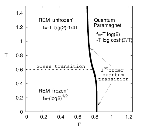
The complete phase diagram of the QREM as a function of and has been obtained in [34] by means of the replica method, and is reported in Fig. 9. The existence of a first order phase transition in (a slight variant of) this model has been rigorously confirmed in [41]. This phase diagram can be obtained via a series of extremely simple arguments [38]:
- 1.
Extreme cases
We start by discussing the two limiting cases (i) = 0 and (ii) .
(i) When the model has a phase transition as a function of the temperature [140], that we already discussed in Sec. 3.3 and we briefly recall here. The micro-canonical entropy density is on the interval of energy densities where it is positive, i.e. with . In consequence a condensation (or glass) transition occurs at the critical temperature : at high temperatures the free energy density is and an exponential number of configurations contribute to the partition function. On the contrary at low temperatures the Gibbs measure is concentrated on a finite number of configurations of energy density , and ; the entropy density then vanishes.
(ii) When the system corresponds to independent spins in a transverse field, i.e. a simple Quantum Paramagnet (QP). As a consequence the free energy reads and the entropy density is the logarithm of a binomial distribution on .
- 2.
Perturbation theory
We now discuss the perturbation theory around these two limiting cases. Consider first a classical configuration with a negative energy density . The energy density of the corresponding eigenstate of can be computed order by order in , treating the transverse field as a perturbation, and this yields:
(51) as typical configurations that are reached by a single spin flip from a low energy configuration of the REM are the most numerous ones, with vanishing energy density (this will be further explained in Sec. 4.3.2).
In the opposite limit , the eigenstate of the pure transverse field are degenerate so we must use degenerate perturbation theory. Consider the space of eigenstates where spins are aligned in the transverse field direction. This space has degeneracy . Here we consider the classical part of the Hamiltonian, as a perturbation. It is easy to show that the restriction of this Hamiltonian to each degenerate subspace is a random matrix, whose elements are Gaussian variables with zero mean and variance . Therefore this is a random matrix belonging to the Gaussian Orthogonal Ensemble (GOE) and its spectrum is the usual semi-circle law with eigenvalues . We obtain that on the QP side, at first order, the energy levels are those of free spins in a transverse field, with exponentially small corrections. See [213] for the second order computation.
The important outcome of these considerations is the vanishing as of the perturbative corrections around the two limits and , hence the energy, entropy and free energy densities are not modified. The free energy density of the QREM is thus , which leads to a first order phase transition when the values of the free energies of the two competing phases become equal. The spectrum and the phase diagram of the model in the plane are shown in Fig. 9.
- 3.
Gap
A good approximation of the minimum gap is given, as in the ordered case, by considering a two level problem similarly to (15) where the space is that spanned by the ground states of the classical part of and of the transverse field, denoted respectively (that corresponds to the classical state of minimal energy) and . The diagonal matrix elements are the perturbed energies. The off-diagonal elements are proportional to the overlap . From this we obtain that and the accuracy of this scaling is shown in the inset of Fig. 9.
The phase diagram of the QREM shares strong analogies with the results obtained in other quantum spin glass models belonging to the RFOT class [212, 35, 37, 36], consistently with the fact that the REM is a good approximation for more complex systems. In all these problems the classical glass transition occurs as a function of the temperature. At the system is in the glass phase and the classical ground state is not extensively degenerate. We stress here that this is a crucial difference with respect to many other optimization problems, like -SAT, where the glass transition also arises at as a function of the density of constraints. In these cases the entropy density is non-vanishing at zero temperature and the transition is an entropic phenomenon. We will show next how the role of entropy can be taken into account in a simple extension of the REM, the random subcubes model we already introduced in Sec. 3.6.
Note the analogy of the computation of the gap in the QREM with the one of the Grover problem discussed in Sec. 2.3.5. However, in the QREM the classical intensive ground state energy has fluctuations of order , which induce similar fluctuations of the location in of the minimal gap. Hence, in this case the optimal schedule discussed in Sec. 2.3.5 for the Grover problem (that is based on the exact knowledge of the location of the minimal gap) cannot be applied and a quadratic speedup is not achieved by the QAA in the QREM. Hence, the behavior of a QAA (as well as that of a classical annealing) is the same as in the ordered case: finding the ground state takes a time , exactly as in an exhaustive search. An annealing over a finite time will lead to an extensive residual energy.
4.3 Level crossings and localization on the hypercube
In sections 4.1 and 4.2, we presented an overview of several simple models that show different phenomenologies: first and second order quantum phase transitions, associated to different scalings of the gap at the transition. Moreover, we announced that some of these models are characterized by phases where the gap is everywhere exponentially small due to an accumulation of level crossings [102, 39, 40]. In this section, we shall give a more detailed description of this level crossing phenomenon.
The approach we shall use here has its roots in the physics of Anderson localization. In [139], Anderson considered a particle hopping on a -dimensional cubic lattice of sites, and subject to a random disordered potential, as a good starting point for the comprehension of transport properties of metals and of the metal-insulator transition. The Anderson model describes an electron hopping in a disordered environment and the Hamiltonian reads
| (52) |
where the first sum runs over the edges of the lattice, i.e. pairs of sites at distance 1, the second sum runs over all sites, is the creation operator at vertex of the lattice, and are i.i.d. random local energies, taken from a given distribution. Anderson showed that, depending on dimensionality and on the strength of the disorder, the eigenstates of the Hamiltonian (52) can be extended or localized in real space [139]. What is particularly interesting for the present discussion is that the spectral properties change completely in the extended or localized regions of the spectrum. Indeed, extended states are typically separated by much larger gaps than localized ones. In the literature on Anderson localization, this is sometimes referred to as level repulsion. Level repulsion is suppressed for localized states exactly because the matrix elements that connect them are much smaller, hence the in Eq. (15) is much smaller leading to smaller gaps. Therefore, one might expect that the presence of avoided level crossings leading to exponentially small gaps could be interpreted as some kind of localization phenomenon [40]. We discuss this point of view in detail in the rest of this section.
4.3.1 A different view on the QREM: the Anderson model on the hypercube
A simple observation is that the transverse field operator has non-zero matrix elements between two states and if and only if the Ising spins configurations and differ on exactly one variable . Considering the configurations as the vertices of the dimensional hypercube, and defining the Hamming distance as the number of different bits between the two configurations and , one can rewrite any Hamiltonian of the form (50) as
| (53) |
where the second sum runs over pairs of neighboring configurations on the hypercube, i.e. such that . In this formulation the QREM discussed in Sec. 4.2.2 is exactly the Anderson model on the hypercube, as the energies are random i.i.d. variables, precisely as the of (52), the transverse field playing the role of the particle hopping term of the original Anderson model.
As we discussed in Sec. 4.2.2, the energies of the QREM provide a disordered environment that induces localization on one of the vertices of the hypercube when the hopping is not strong enough. This is shown by the fact that the low energy eigenstates at small enough coincide with the classical ones, hence with , at all orders in perturbation theory for , see Eq. (51) [38]. The crucial difference with the Anderson model is that here, the delocalization transition coincides with the first order phase transition, and it happens via a level crossing between the localized and extended ground state. Moreover, in the localized (small ) phase, no level crossings are observed between different states; this is clearly due to the fact that the energies of the lowest eigenstates do not depend on , again due to Eq. (51) [38].
The analogy between the QREM and the Anderson model is strongly appealing for the physicists community since it brings the field of quantum information and the one of Anderson localization of interacting systems in close contact [40]. On the other hand, the localization in the QREM is “extreme” in the sense that in the localized phase the eigenstates of the Hamiltonian coincide with the classical states. This is due to the fact that the Hamiltonian is non-local and flipping a spin typically costs an extensive energy.
Therefore, several interesting questions remain open. In local Hamiltonians (Sec. 2.2.2), one expect that for finite , states are always delocalized over an exponential number of states of the computational basis (see the discussion in [214]). What is then the meaning of many-body localization? Is it possible to observe, in more general models, level crossings in the “localized” phase? Does delocalization always happen through a first order transition? And finally, what happens when the classical ground state is exponentially degenerate, unlike in the QREM? In the following we try to answer some of these questions.
4.3.2 A mechanism for level crossings between localized states
Let us first consider the case of local Hamiltonians in the sense of Sec. 2.2.2. A mechanism that induces level crossings between localized states was proposed independently by Altshuler et al. [40] and by Amin and Choi [39]. It relies on the fact that in optimization problems with local interactions, the diagonal energies are not uncorrelated as in the QREM. Therefore, a careful choice of the classical energy function can lead to level crossings. We now review this construction.
In [40], a classical random energy function that is a sum of local interactions was considered (namely, the Exact Cover problem defined in Sec. 2.1.1). The analysis starts by choosing an instance of the problem with clauses, such that there are at least two isolated (i.e. separated by an Hamming distance of order ) solutions and of all the clauses. These configurations represent degenerate eigenvectors for . However, as soon as the two ground state energies must split. Let us call and the two eigenvectors that transform continuously into and for , and and the corresponding energies.
The splitting of the two solutions can be computed using perturbation theory for small enough , as we already did for the QREM. One can write for any given non-degenerate classical eigenstate :
| (54) |
with some coefficients . The effect of the presence of two degenerate solutions will appear only at order if the two solutions and have extensive Hamming distance, and therefore it was neglected in the discussion [40]. Let’s look to the first order as an example. It has the form
| (55) |
Fig. 10 highlights the crucial ingredient in the construction of Amin and Choi [39] and of Altshuler et al. [40], and compares it to the QREM. In the latter, the classical energies are uncorrelated and for low energy eigenstates, the coefficient turns out to have a finite limit for . This is because a low energy configuration is connected by a single spin flip to configurations (hence there are terms in the sum), but those typically have an extensive energy difference above it (hence the denominator is of order ). Considering intensive energies, the correction is therefore of order as given in Eq. (51). The crucial difference for correlated energies that are sums of local terms is that a spin flip always leads to a finite energy difference with respect to the starting point. Therefore, the denominators in the perturbative expansion are of order 1, and is of the same order of the classical energy. Extending the argument to higher orders one easily sees that all orders in perturbation theory are proportional to , if the energy is the sum of local interactions, and therefore contribute to the -dependence of the energy levels.
Hence, recalling that both and are assumed to have zero classical energy and calling , we have:
| (56) |
It was argued in [40] that for random problems the coefficients have the same average over the disorder; hence, has zero mean and naturally one can assume that . This leads, on average, to
| (57) |
where are finite for large . Eq. (57) shows that, if the first non-zero coefficient is negative, one can find a small enough such that for any finite . In fact,
| (58) |
Now, we can add an -th clause to the problem and fix in such a way that the new clause introduces at most a penalty on the classical energy (in the Exact Cover problem, ). Then, it still holds that . At the same time, there is a finite probability that the additional clause will be satisfied by but not by , so that . Because in the Hamiltonian there are no particular symmetries, the matrix element between and will be non-zero and the introduction of the additional clause induces an avoided level crossing, as in Eq. (15).
Once again, the avoided level crossing is associated with an exponentially small gap because by assumption the two solutions have an Hamming distance of order , hence they can only be connected at order in perturbation theory, leading to a matrix element of order , i.e. exponentially small. It is important to stress that in this construction the crossing happens for , hence at very small in the thermodynamic limit. For this reason, these crossings have been called perturbative crossings in the literature [40, 41, 215]. This scaling was not clearly found in the numerical experiments, but this was attributed to the small exponent, visible only for large [40].


A similar phenomenon was discussed by Amin and Choi [39]. Their construction is based on a system whose classical energy function has a deep but narrow energy minimum, and a secondary local minimum which is higher in energy but wider (see Fig. 10, right panel). This means that around the secondary minimum, flipping a spin costs less energy. The denominators in the perturbation theory, Eq. (55), are smaller around the secondary minimum than around the global one. In turn, the secondary minimum lowers its energy more quickly under the action of the transverse field and eventually crosses the classical minimum.
The analysis of [40, 39] points out an important mechanism that can induce level crossings representing a serious bottleneck for quantum algorithms, that is a missing ingredient of the QREM, which is the simplest Anderson-like model of localization on the hypercube: namely, the fact that in systems with local interactions the diagonal energies are correlated, and most importantly a single spin flip always lead to a finite change in the classical energy, which is not the case in the QREM. Thanks to this, the energy densities of the classical eigenstates have a non-trivial perturbative expansion in . Therefore, one can find particular realizations of the disorder, such that the energy of a classically excited state decreases faster, as a function of , than the ground state energy, leading to a crossing at small .
This mechanism is for the moment only understood in perturbation theory (whose validity for these systems has been criticized [216]), and therefore it holds whenever perturbation theory holds, that is, if at small enough the full eigenstates of the quantum problem remain close enough to the classical eigenstates. This is what has been called a “many-body localization” phenomenon in [40]. The other important ingredient is a very particular construction of the instances of the problem, that admit only two solutions. But, as we already discussed in Sec. 3.9, typical instances of generic random optimization problems, even close to the satisfiability threshold, have an exponentially large number of solutions, and so we expect that non-degenerate perturbation theory should not hold, and the spectrum should be much more complex. Therefore we would like to understand what happens generically in problems that exhibit multiple and not necessarily isolated solutions. In particular, do the avoided crossings remain finite and isolated in (hence leading to singularities in the ground state energy for ) or do they proliferate and accumulate, leading to a continuum of level crossings and a gapless phase? The latter question is particularly important, because it has been argued that a finite number of level crossings can be eliminated by suitable redefinitions of the quantum Hamiltonian [217, 218, 42, 219, 43, 215, 41]. We will address it in the next section.
4.4 Level crossings and the role of entropy: the random subcubes model

Motivated by the previous discussion, we now analyze a simple extension of the REM that takes into account the role of the massive ground state degeneracy: the Random Subcubes Model (RSM) introduced in its classical version in [172]. Given that this model can be fully solved and reproduces most of the phenomenology we are interested in this section, we will discuss its properties in some detail. Some of these results have been published in [47].
The cost function (or problem Hamiltonian ) of the classical model has been defined in Sec. 3.6. We recall here that there are random clusters (that have the topology of sub-hypercubes of the total Hilbert space, hence the name subcubes); when these clusters are disjoint (the regime of interest here) configurations belonging to a cluster have a random classical energy . Configurations that do not belong to any cluster have classical energy and we assume that . The classical properties of the model have been discussed in Sec. 3.6, where it was shown that at large enough the space of low energy configurations is decomposed into a set of disconnected clusters separated by large energy barriers. This is illustrated in Fig. 11 that should make the difference between the REM and RSM evident. All our analysis of the Quantum RSM (QRSM) will be restricted to the region when the clusters are well disjoint (see Sec. 3.6).
The main result of this section will be that quantum fluctuations, combined with the cluster structure, give rise to a series of level crossings induced by a combined energetic-entropic effect. Before going into the details, it is useful to give an overview and illustrate the way in which the model will be analyzed. In Sec. 4.4.1 we will discuss the spectrum of the clusters at finite in the limit . In this limit the Hamiltonian is block diagonal, each block corresponding to one cluster. The spectrum is characterized by true level crossings between states belonging to different clusters. The level crossings are due to the interplay of the classical energy and the classical entropy of the clusters. Quantum fluctuations, indeed, favor more entropic clusters. In Sec. 4.4.2 we will consider the case of finite (still at finite ). A finite reintroduces a lot of additional states that have to be taken into account. They allow to connect the clusters by single spin flips, therefore the Hamiltonian is no longer block diagonal. We will treat this situation by perturbation theory and variational arguments to show that a finite (large) induces only minor modifications with respect to the infinite case. In Sec. 4.4.3 we will investigate the low energy spectrum obtained by exact diagonalization for finite system sizes, and show that it is characterized by several avoided level crossings. In Sec. 4.4.4 and 4.4.5 we will consider the thermodynamic limit . In Sec. 4.4.4 we will focus on the ground state, at . We will show that there is a first order phase transition that separates a Quantum Paramagnetic (QP) phase, at large , from a Spin Glass (SG) phase, at smaller , like in the QREM. In the spin glass phase the ground state continuously changes from one cluster to the other as a function of , because of the level crossings between different clusters; the latter accumulate for giving rise to a unique SG phase, and are therefore distinct phenomena with respect to the first order transition. Finally in Sec. 4.4.5 we will consider the case : we will show in particular that quantum fluctuations promote the glass transition. In Sec. 4.4.6 we summarize and we comment the results.
4.4.1 Spectrum of the cluster Hamiltonian
We will now study the spectrum of the quantum Hamiltonian as a function of , and from now on we focus on the region where clusters are well separated (see Sec. 3.6), which is the most interesting for our purposes. The computation of the spectrum for is more complicated, because in this region the clusters have overlaps and the arguments below do not apply straightforwardly (although they might be generalized for where the overlaps are exponentially small [172]). A schematic example of the Hamiltonian describing a finite system with three clusters in the regime where the clusters are well-separated is shown in Fig. 12.

Remember that we call the set of all classical configurations that belong to at least one cluster ( being the Hamiltonian of a cluster), and have therefore classical energy extensively smaller than ; configuration that do not belong to have energy (and are described by the Hamiltonian ). The total Hamiltonian is . We consider first the (“hard”) limit where is infinite for the states that do not belong to : then we can project out these states from the Hilbert space and look to the restriction of on , which contains states. Because the matrix only connects configurations at unit Hamming distance, and different clusters have distance of order , the Hamiltonian has no matrix elements connecting different clusters. Therefore we can diagonalize separately in each cluster. The restriction of to a given cluster with free spins is equal to plus the Hamiltonian of uncoupled spins in a transverse field, its spectrum is hence made of levels
| (59) |
each times degenerate. In particular the lowest level has energy per spin , therefore the energy of clusters with larger entropy decreases faster with . In this regime then one expects level crossings between states belonging to different clusters. In the situation where bigger clusters at have larger classical energy, which is the case for most random optimization problems, the level crossings concern the ground state and at each crossing corresponds to a global rearrangement of the system. A simple example of a spectrum in the limit regime for a finite system containing three clusters is shown in the left panel of Fig. 13. Note that as long as the clusters are well separated, due to the limit, there are no corrections in the size of the system. The crossings are not avoided and the degeneracy of the states is not removed, due to the complete independence of the Hamiltonian sectors describing each cluster.


(Left panel) Spectrum in the case. To each cluster corresponds the spectrum of free spins in a magnetic field.
(Right panel) Partial spectrum for finite obtained by exact diagonalization, with a zoom on the ground state in the inset. Green lines are the results of second order perturbation theory, the blue line is . At small the low energy spectrum is in good agreement with that at . For larger values of , avoided level crossings appear (marked by red arrows). The crossings at smallest involve different clusters. The largest crossing, instead, involves the ground state of the spectrum connected to the classical low energy spectrum (set ) and the ground state of the -band; this crossing becomes a true first order phase transition in the limit.
4.4.2 Quantum paramagnetic state
Next, we consider a “soft” version of the model in which is finite (still with ). Therefore now is defined on the full Hilbert space . In this case, in addition to the energy levels discussed above (that we shall refer to as the -band), there exists another set of levels (the -band), whose energy is expected to be of order at small .
For the states in the -band we use perturbation theory in . As soon as the transverse field is switched on a first order correction in to the states in the -band is present. This correction comes from the partial lifting of the degeneracy within the cluster and it is given by the spectrum in Eq. (59). A second order correction is induced by the presence of the -band at finite . In order to compute it one can apply perturbation theory assuming as unperturbed basis the one that diagonalizes the perturbation inside each cluster. In particular we are interested in the correction to the lowest energy level in the clusters whose state is given by all free spin polarized in the direction of the field. Then the correction is
| (60) |
and at any finite order the correction to the energy per spin is , so it vanishes in the thermodynamic limit. This mechanism is similar to the QREM and is due to the fact that states at the boundary of the clusters have extensive larger energy.
To study the lowest energy level in the -band it is convenient to rewrite the Hamiltonian in the following way:
| (61) |
where is the identity and indicates the projector over the cluster . acts on the entire Hilbert space while acts only on the subspace spanned by the clusters. This form aims to interpret as a “perturbation” over which describes a system of free spins in a transverse field (with a shift in the energy). However the “perturbation” is not in the strength of the energy, which may be large, but in the number of states that are involved. Note, in fact, that Rank()Rank(), being Rank() and Rank(). This, together with the fact that the perturbation matrix is positive defined (it shifts some states all in the same direction) allows to apply the results of small rank perturbation analysis [220] in order to study . From these results we can safely say that
| (62) |
where and are respectively the -th eigenvalues of and , and we assume when . In particular when is small, is larger than all the energies in the -band. This implies that
| (63) |
The results from small rank perturbation (62) also shows that the spectrum of the -band is close to the one of free spins in transverse field with classical energy :
with degeneracy close but not equal to . We expect that the unperturbed ground state of , describes well the lowest energy level of the -band and remains unaffected by the presence of the states in for all except from the region where it crosses the spectrum of . The reason for this comes from the intuition that in absence of the spectrum of is highly degenerate, especially in the middle of the band. Then, also comforted by the results of exact diagonalization, we expect that the states that recombine the most in order to create the -band when is applied, are those belonging to the more degenerate part of the spectrum. On the contrary, is made of all spins aligned along without degeneracy and thus it is weakly perturbed by . A rigorous study of this energy level is not possible, but we can use a variational argument to understand its behavior. The state has exponentially small overlap with any state in the -band and thus it gives an expectation value of equal to for some . If we interpret this as a variational upper bound on the true ground state of the -band we get:
| (64) |
Combining (63) and (64) we obtain
| (65) |
and the corresponding eigenvector remains up to exponentially small corrections the same , which is uniformly extended in the basis .
4.4.3 Exact diagonalization results
We checked these predictions for the spectrum by means of exact diagonalizations for a system made of spins. The results are shown in Fig. 13, in the right panel. There we have plotted the spectrum of a system made by three clusters characterized by classical energy and entropy and . The plot shows that for small the states in the -band do not affect those in the set , whose spectrum is in good agreement with that at , in the left panel. At larger , avoided level crossings first appear between the ground states of different clusters. Finally, an avoided crossing happens with the ground state of the -band, whose slope in is much larger due to the big entropy which characterizes this sector. We have also plotted in green the analytical result that we obtain up to second order in perturbation theory for the lowest energy level of each cluster and in blue the energy of the quantum paramagnetic state. We see that the true ground state, crossing after crossing, well interpolates between all these curves. Since the clusters have Hamming distance proportional to , we expect all these crossings to be avoided at finite producing exponentially small gaps [39, 40, 41].
4.4.4 Level crossings in the thermodynamic limit


(Left panel) Energy of the SG ground state [Eq. (66), full line] and of the QP state for (dashed line). A first order transition between the two states happens at . (Inset) Level crossings in the SG state. For better readability we plot [Eq. (66), full line] and show the energy of two different clusters with (dot-dashed lines).
(Right panel) Transverse magnetization as a function of for the same parameters. The first order phase transition between the SG and the QP is manifested by a jump in , shown by a vertical dotted line. The value of for the SG is the solid black line, while that of the QP is the dashed blue line. Note that the latter is bigger because it corresponds to a more entropic phase.
We discuss now the zero temperature phase diagram of the model for and . Following Sec. 3.6, to get a meaningful thermodynamic limit, the number of clusters of energy is set to , where is an arbitrary increasing function of (as in most random optimization problems). We assume that so the total number of clusters in is still . As discussed in Sec. 3.6, the complexity of clusters of energy and entropy is , and it vanishes at which is also an increasing function of . The -band, or spin glass (SG), ground state energy is
| (66) |
The minimum is in as long as . Above this value, the minimum is in a different for each value of : in this region the ground state changes abruptly from one cluster to another upon changing by an infinitesimal amount, similarly to what is called temperature chaos in spin glasses [184, 186]. Note that in some relevant cases the slope of in is infinite, therefore and level crossings happen at all .
The energy crosses the SG ground state given by Eq. (66), giving rise to a first order phase transition between the SG and the QP [38, 34, 35, 36, 37, 48] at a critical . As a consequence, the transverse magnetization has a jump at the transition [48] (see the right panel of Fig. 14). Note that , thus the transverse magnetization is determined by the entropy of the ground state, and the entropy of the -component is much larger than those of the clusters.
4.4.5 Finite temperature: the condensation transition

The previous analysis shows that in the region the perturbation has a dramatic effect. At , most of the states in belong to one of exponentially many small clusters, while at any the few largest clusters of entropy have the smallest energy. This is related to the fact that the presence of a transverse field introduces a correction to the energy that favors the more entropic clusters. A more complete picture is obtained by studying the model at finite temperature (recall that the classical model at finite temperature was studied in Sec. 3.6.3). It is convenient to separate the contribution of the two parts of the spectrum (the -band corresponding to the SG phase and the -band corresponding to the QP phase) to the partition function, , with :
Of course, reduces to the classical partition function in Eq. (39) for . The free energy is , analogously to what was found in [38] for the QREM (see the discussion in Sec. 4.2.2), with and
| (67) |
The first order transition happens when the free energies and cross, while the condensation transition happens when the maximum in Eq. (67) is attained in for the first time. In Fig. 15 we plot the lines versus for several temperatures. We observe that in the limit , the lines shrink to the horizontal axis and the system is in the condensed phase for any . The first order transition to the QP phase happens for larger values of at fixed temperature, and it is reported in the plot for .
4.4.6 Summary
Before presenting a more general perspective on random optimization problems, let us summarize the results of this section. We introduced a simple toy model of a quantum optimization problem, the QRSM based on the RSM of [172]. In the classical case , the model captures the essential structure of the space of solution of random optimization problems, and displays several phase transitions that are present also in more realistic problems such as -SAT, at least at large . We explored the consequences of this complex structure on the spectrum of the quantum Hamiltonian at , and we showed that: (i) Quantum fluctuations lower the energy of a cluster proportionally to its size. (ii) Because the energy and the entropy vary from cluster to cluster, level crossing between different clusters are induced as a function of in the SG phase, due to a competition between energetic and entropic effects. These crossings accumulate for in a continuous range of , giving rise to a complex SG phase characterized by a continuously changing ground state and an everywhere exponentially small gap. (iii) At large the SG phase undergoes a first order transition towards a QP phase, corresponding to the complete delocalization of the ground state in the computational basis . (iv) At finite temperature, there is a line of condensation transitions that shrinks to at low temperatures: indeed, at zero temperature the condensation transition becomes abrupt. While at the space of solutions is dominated by an exponential number of clusters of intermediate size, for any the biggest clusters contain the ground states.
4.5 Phase transitions in quantum optimization problems: an attempt towards a general perspective
Overall, the discussion of the previous sections shows that the low energy spectrum of quantum optimization problems can be very complex, and characterized by different level crossings: internal level crossings in the SG phase, or the crossing between the SG and the QP giving rise to a first order phase transition. Moreover, both entropic and energetic effects are important.
Yet the previous discussion was based on a series of toy models (such as the QREM or the QRSM) or on the analysis of extremely simplified instances of random optimization problems. These problems were basically constructed ad hoc to exhibit the desired phenomenology. The next task is therefore to demonstrate that these phenomena indeed happen in typical instances of realistic random optimization problems, such as those defined in Sec. 2.1.1. This will be the subject of Sec. 6, but it requires the introduction of sophisticated quantum statistical mechanics tools that we will discuss in Sec. 5. Before proceeding, in this section we want to complete the picture by presenting coherently what are the expected properties of the spectrum of generic random optimization problems.
 |
 |
 |
 |
As was explained in Sec. 3, the classical energy landscapes of several random optimization problems have been recently characterized in much detail, thanks to important developments in the analysis of classical spin glasses [32, 129, 152, 125, 136, 137]. These studies show that the classical energy is characterized by many “valleys” at the bottom of which local minima are found; we are now able to obtain a quite detailed quantitative characterization of the shape of these valleys [188]. We can use as running examples the random regular XORSAT problem, in the satisfiable phase where solutions exist, which is a representative of the class of locked models discussed in Sec. 3.9, and the random -SAT problem, which instead displays (for ) all the transitions discussed in Sec. 3.7. In Fig. 16 we sketch pictorially the energy per spin as a function of the configuration for those models, and compare with the previously investigated toy models, the REM and RSM. The picture shows some very general aspects of mean field spin glasses, that are shared by all the models considered here:
- a.
The energy landscape contains many local minima.
- b.
The distance between low energy configurations belonging to the basin of attraction of different minima is .
- c.
The height of the energy barriers separating two different minima is .
At the same time, there are some crucial features that are model dependent also within mean field models:
- d.
The number of configurations around a given local minimum might be exponentially large (the entropy is positive) or not (the entropy is zero).
- e.
The (intensive) energy change associated to a spin flip starting from a low energy configurations can be either or . The latter case is the rule for Hamiltonians that are the sum of local terms, and in this case the “steepness” of the energy around a local minimum can depend on the minimum itself.
Based on the previous analysis of toy models, we expect that each low energy cluster of the classical energy function gives rise, under the action of a quantum term like a transverse field, to a set of states (whose size roughly corresponds to the classical entropy of the cluster), with an energy density of the form
| (68) |
The coefficients of both terms depend on the shape of the classical energy around the local minimum. It was shown explicitly for the QRSM that the coefficient of the linear term is directly proportional to the intensive entropy of the cluster. Therefore, if local minima are exponentially degenerate, this coefficient is with respect to , and its fluctuations from cluster to cluster are also . Moreover, it was shown in Sec. 4.3.2 that the coefficient of the quadratic term depends on the neighborhood of the local minimum. Fluctuations of the latter coefficient among different minima are in the example of [40] but might be in other models.
The cluster to cluster fluctuations of the quantum corrections will generically lead to avoided level crossings. Because of the huge number of different clusters, it is reasonable to expect that these crossings will accumulate for leading to an everywhere gapless spin glass phase, as it was shown explicitly for the QRSM. This phase will cease to exist at large enough , when the completely delocalized state, corresponding to the quantum paramagnetic phase, will cross the cluster ground state. Generically we expect this crossing to become a first order transition in the thermodynamic limit (as in the QREM and in the QRSM), but the transition might also be of higher order depending on the model. We will discuss concrete examples in Sec. 6. In summary, we expect generic problems to display a complex spin glass phase for small , separated by a quantum critical point from a simple quantum paramagnetic phase.
5 Methods
The aim of this section is to review various methods that can be used to investigate quantum spin glass models. We will give a particular emphasis to the methods that are most efficient to treat the quantum versions of the family of random optimization problems introduced in Sec. 2.1.1 and Sec. 3.1. We will use these methods in Sec. 6 to obtain results on specific models such as the XORSAT and coloring problems. This section is organized as follows: we will start in Sec. 5.1 by introducing the classical cavity method, a framework that has been developed to study random ensembles of optimization problems and which has led to the understanding of their complex phenomenology, that we explained in Sec. 3.7. The next three sections (5.2, 5.3 and 5.4) will be devoted to different approaches to the generalization of the classical cavity method to quantum models. Finally in sections 5.5 and 5.6 we will give some details on some more standard numerical methods, such as exact diagonalization and quantum Monte Carlo, that have also been used to obtain important informations on these problems. Before entering in the core of the discussion let us give a more detailed overview of the rest of this section.
As already explained in Sec. 3.2, disordered mean field models [32] can be roughly classified in two categories: fully connected ones, where each degree of freedom interacts weakly with all others, and finitely connected ones, with a finite number of strong interactions for each degree of freedom. The replica method has been originally devised for the former family, most notably for the Sherrington-Kirkpatrick model [142]. Its extension to the finite connectivity case [151, 129] has been more conveniently reformulated in terms of the cavity method [152], and applied in particular to random ensemble of Constraint Satisfaction Problems (CSP) [126, 130]. The classical cavity method is by now a well established technique, with many presentations in original research papers [152, 221] and in a textbook [137], and rigorous proofs of validity in some cases [131, 132, 222]. For the sake of completeness, in Sec. 5.1 we provide a quick survey of the classical cavity method, before turning to the specificities of its quantum version. In this section we also discuss the general definition of random graph models and the key concept of replica symmetry breaking.
Several quantum extensions of the cavity method have been recently proposed in a series of papers, able to treat for instance spin 1/2 models in presence of a transverse field. Roughly speaking, these methods can be divided in three groups. Path Integral Quantum Cavity (PIQC) methods exploit a path integral representation in order to map the quantum problem into a classical one and then make use of the classical cavity method [223, 224, 225, 48]. Operator Quantum Cavity (OQC) methods work directly with quantum operators [226, 227, 228, 229, 230]. Finally, Variational Quantum Cavity (VQC) methods propose a variational ansatz for the ground state wavefunction that can be represented in terms of a set of local parameters, and then use the classical cavity method to optimize the energy of the variational state [231].
PIQC is at the moment the only analytical method that was used to obtain concrete results on one of the random CSP defined in Sec. 2.1.1, namely XORSAT in presence of a transverse field [48]. The goal of Sec. 5.2 is to explain the technical details of the PIQC at the level of one step of replica symmetry breaking, that is needed for the solution of these problems [48], and to generalize it to arbitrary discrete quantum degrees of freedom33 3 Note that the PIQC has also been used in a condensed matter context, namely to investigate quantum glassy phases of disordered interacting bosons on random lattices; a detailed explanation of the method in this case can be found in [232, 198]. . We will rely on this method in Sec. 6 to present detailed results on the XORSAT model [48] and original results on the coloring problem.
The main drawbacks of PIQC are that i) as any path integral sampling method, it is restricted to Hamiltonians that are not plagued by the “sign problem” (or in other words that admit a path integral representation where the trajectories have positive weights), ii) it does not allow to work exactly at , but only to perform an extrapolation to from finite temperatures and iii) the resulting functional equations have to be solved using a statistical representation, that is affected by fluctuations and/or finite size (of the representation) effects. These drawbacks could in principle be overcome by working directly with operators. In Sec. 5.3 we will describe several attempts to construct OQC methods [226, 227, 228, 229, 230]. In Sec. 5.4 we will describe VQC methods that are specifically designed to obtain direct information at [231]. Although these attempts are extremely promising and already allowed to obtain very interesting results for simple ordered and disordered models, it turns out that for the moment they are too computationally demanding to be used to solve the problems of interest here (e.g. the XORSAT problem). This will be discussed in Sec. 6.
5.1 The classical cavity method
5.1.1 Factor graph models
Let us recall some definitions of Sec. 2.1.1 and put them in a more general context. We consider a model with degrees of freedom taking values in a finite alphabet , for instance for Ising spins. We denote the global configuration, and for a subset we write the configuration of those variables. The model is further defined by its energy function , that contains interactions labeled by :
| (69) |
For each of the interactions denotes the set of variables that interact through with the energy term ; a convenient representation of such an energy function is provided by factor graphs [233], see left panel of Fig. 17. Each variable is associated to a circle vertex (variable node), while interactions are represented by squares (function nodes), an edge being present between interaction and variable if and only if the value of depends on , i.e. if and only if . We shall also use the notation for the set of interaction nodes linked to the variable , and call graph distance between two variables and the minimal number of interactions in a path along the factor graph between and .


The Gibbs-Boltzmann measure at inverse temperature of the model can be written as
| (70) |
where the partition function ensures the normalization of the probability law, and where the interaction weights are given by . For future convenience we shall treat a slightly generalized case with weights on the variables. For Ising spins, the latter can be thought as originating from local magnetic fields.
Let us assume momentarily that the factor graph representing the model under study is a tree. Then the problem of characterizing the measure (70) and computing the associated partition function can be solved exactly in a simple, recursive way. One introduces on each directed edge from one variable to an adjacent function node a “message” , which is a probability measure on the alphabet , that would be the marginal probability of if the interaction were removed from the graph. These messages are easily seen to obey the recursive (so-called Belief Propagation) equations depicted on the right panel of Fig. 17,
| (71) |
with ensuring the normalization of the law .
On a tree factor graph there exists a single solution of these equations, which is easily determined starting from the leaves of the graph (for which the empty product above is conventionally equal to 1) and sweeping towards the inside of the graph. Once the messages have been determined all local averages with respect to can be computed, for instance the marginal law for a single variable and for the set of variables around one interaction read respectively
| (72) | |||||
with and defined by normalization. Moreover the partition function can be computed as
| (73) | |||||
5.1.2 Random ensembles
In the definition of the energy function (69) and of the associated Gibbs-Boltzmann measure (70) we considered a single realization of the model. We turn now to random ensembles of such models. Their definition involves a probability law on the integers, that we shall denote ; for simplicity of notation we assume that all interactions involve the same number of variables. The factor graphs are then supposed to be chosen uniformly at random among those with variables and such that a fraction of variables is involved in interactions. The number of interactions is then , with related to the degree distribution by the relation . This definition is an hypergraph generalization of the random graph models with prescribed degree distribution, studied for instance in [234]. The Erdős-Rényi construction described in Sec. 3, where the interactions are chosen uniformly at random among the possible ones, is essentially equivalent to the one just described, with the Poisson distribution of mean . In the definition of the random energy function we also assume that the interaction and variable weights and are chosen independently at random from two probability laws. We will denote the average with respect to the whole construction; the main objective in the field of disordered systems is the computation of the average free energy density in the thermodynamic (large size) limit,
| (74) |
as the free energy is a self-averaging quantity, which yields all relevant thermodynamic quantities by suitable derivatives with respect to its parameters.
The cavity method allows to compute the thermodynamic limit of the free energy density for models defined on random graphs. It exploits some properties of these random graphs, in particular their tree-like character: in the thermodynamic limit these random graphs converge locally to random trees. This means that the neighborhood within a fixed graph distance of an arbitrary variable node is, with a probability going to one as with fixed, a tree. The latter can be described by and an associated distribution . Indeed the reference node will have interaction nodes around it with probability . Then each of the variables at distance 1 from will have a number of descendants drawn independently from the law , and so on and so forth until generations of vertices have been drawn (all degrees are drawn from except the first one with ). One can notice that is the degree distribution of a variable node chosen uniformly at random, while corresponds to the selection procedure where one edge of the factor graph is chosen at random, say between and ; then belongs to interaction besides with probability .
We explained above how statistical mechanics models defined on trees could be solved recursively. On the other hand we have just recalled that random graphs are locally tree-like; the cavity method is a set of prescriptions on how to exploit the local properties of the random graphs to make global predictions on the free energy density. Depending on the models, in particular on the amount of frustration between the variables they induce, different level of sophistications of the cavity method are necessary.
5.1.3 Replica symmetric cavity method
The simpler one, exact for instance for ferromagnetic, unfrustrated, models, goes under the name of Replica Symmetric (RS). In that case there exists a single pure state (or a small number of them simply related by explicit symmetries of the model) in the Gibbs measure, which enjoys in consequence spatial correlation decay properties. The effect of the long loops which are present in the random graphs is then negligible in the thermodynamic limit, only providing a self-consistent boundary condition. The recursive equations (71) valid for a single tree factor graph are given a probabilistic meaning to describe the thermodynamic limit of random graphs. More precisely, the order parameter of the RS cavity method is , the probability (over the disorder) that the messages in Eq. (71) (which are themselves probability distributions on ) are equal to . obeys a self-consistent functional equation, which is more simply written in a distributional form as
| (75) |
In this equation all the ’s are drawn independently from , and denotes the equality in distribution between random variables. Moreover is drawn according to the law , the and ’s are independent copies of the variable and interaction random weights, and the function in the r.h.s. is defined by
| (76) | |||||
ensuring the normalization of . The RS prediction for the free energy in the thermodynamic limit is then
| (77) | |||||
where the expectation is with respect the independent choices of (with the degree distribution ), of the ’s (according to the law ) and of the random weights and ’s, and where the contribution of the variable and function nodes are defined by
| (78) | |||||
One can also obtain the disorder average of local observables, for instance the average of the marginal probability for a single variable reads
Other thermodynamic observables can be obtained in a similar fashion; one way to derive their expressions is to observe that the expression (77) for the free energy is variational, in the sense that the stationary conditions with respect to coincide with the self-consistent condition of Eq. (75). In consequence one can use the partition function as a generating function of the observables to be computed, and take only explicit derivatives with respect to their conjugated fields in (77).
5.1.4 Replica symmetry breaking
The assumption of correlation decay that underlies the RS cavity method can fail in presence of frustration, for instance in the case of random CSP with , the clustering transition. Indeed the configuration space of these models gets fractured in a large number of pure states, called clusters in the context of random CSP, as explained in Sec. 3.7 and sketched in Fig. 7. The correlation decay hypothesis only holds for the Gibbs measure restricted to one pure state, not for the complete Gibbs measure. This complication can be handled by the cavity method with “replica symmetry breaking” (RSB). It amounts to make further self-consistent hypotheses on the organization of these pure states, and on the correlated boundary conditions they induce on the tree-like portions of the factor graph. Inside each pure state the RS computation holds true, the RSB computation is then a study of the statistics of the pure states. Let us explain how this is done in practice at the first level of RSB (1RSB cavity method). The partition function is written as a sum over the pure states , , where is the partition function restricted to the pure state (recall the decomposition of Eq. (25)). It can be written in the thermodynamic limit as , with the associated (internal) free energy density. One further assumes that the number of pure states with a given value of the internal free energy density is, at the leading exponential order, , where is called the complexity, or configurational entropy. The latter is assumed to be a concave function of , positive on the interval . In order to compute one introduces a parameter (called Parisi breaking parameter) conjugated to the internal free energy, and the generating function of the as . In the thermodynamic limit its dominant behavior is captured in the 1RSB potential ,
| (79) |
where the last expression is obtained by a saddle-point evaluation of the sum over . The complexity function is then accessible via the inverse Legendre transform of [235], or in a parametric form
| (80) |
where denotes the point where the infimum is reached in Eq. (79).
The actual computation of is done as follows. One introduces on each edge of the factor graph a distribution of messages, which is the probability over the different pure states that , where are the messages that appear in Eq. (71). Because fluctuates from instance to instance, the order parameter now becomes the distribution of with respect to the disorder, which we call and is solution of a self-consistent functional equation written as
| (81) |
Similarly to the RS case the ’s are independent copies drawn from , and the random weights and are also independently generated. The r.h.s. of this equation stands for:
| (82) | |||||
with and defined above in Eq. (76), and is the Parisi parameter. From the solution of this equation one computes the 1RSB potential via an expression similar to (77), namely
| (83) | |||||
with the functions and defined in Eqs. (78), (78). As in the RS case this expression is variational, the implicit dependence of on the various parameters ( in particular) can be discarded when computing derivatives. Various physical situations translate in different behaviors of the 1RSB equations.
- 1.
It can happen that only trivial solutions of (81) exist, i.e. the ’s are supported on a single value of . It is then easy to check that this random obeys precisely the RS equation (75), and that the 1RSB potential is equal to the RS prediction for the free energy of Eq. (77), for all values of . This is the translation of the existence of a single pure state, in which case the whole 1RSB machinery reduces to the RS case. This case is realized at high temperatures/low connectivity parameter , i.e. on the left of the line of Fig. 8. In more physical terms it corresponds to a “liquid” phase, for instance the high temperature phase of the fully connected -spin model described in Sec. 3.4.
- 2.
If on the contrary non-trivial solutions of the 1RSB equations appear, one has to investigate them more carefully in order to obtain the 1RSB prediction for the free energy density. From the definition of one would naturally take for it. This is indeed the case, provided the corresponding complexity is positive, in other words if . The physical interpretation is that an exponential number of pure states contribute to the Gibbs-Boltzmann measure, each with an internal free energy density . It turns out that in this case the prediction coincides with the RS one; this form of replica symmetry breaking is not seen in the thermodynamic properties of the model, yet it has drastic consequences on its dynamics [236, 179]. Such a phase is usually called for this reason a dynamic 1RSB (d1RSB) phase, and is realized in the fully connected -spin model in the intermediate temperature regime , or more generically for diluted mean field spin glasses in the part of their phase diagram enclosed by the lines and (see Fig. 8).
- 3.
If there are non-trivial solutions of the 1RSB equations, but with , one has to find the value which solves the equation , i.e. , and the 1RSB cavity method predicts that the free energy density is precisely this value . In more physical terms this is called a condensed (or true 1RSB) phase, many pure states exist in the system yet only the sub-exponentially numerous ones with do contribute to the thermodynamic behavior of the system, as for instance in the phase of the fully connected -spin model.
As far as the free energy density is concerned, one can give a general formula that encompasses and summarizes the three cases above: it is given by the maximization of the potential with respect to ,
| (84) |
5.1.5 Population dynamics
In general there is no hope to find an analytical solution of the cavity equations, neither at the RS level (75) nor at the 1RSB level (81). These equations are however amenable to a numerical resolution in a relatively simple way.
Let us first consider the RS case. The variables are probability distributions over the discrete space , each of them can thus be represented by real numbers (thanks to their normalization). In particular for Ising spins a single real is enough, that can be interpreted as an effective magnetic field acting on a spin. In the RS equation (75) the unknown is , a probability distribution over such effective fields. A convenient way to represent it numerically [237, 152] is to use a sample, also called population, of representative fields, i.e. to write
| (85) |
This representation thus uses a number of representants , each of them encoded as a single real for Ising spins, or real numbers in the generic case, and is obviously more and more accurate as gets larger. As the equation (75) has the form of a fixed point condition, it can be solved by iteration: one starts from an arbitrary initial assignments of the sample , plugs the representation (85) in the r.h.s. of (75), and constructs a new set that represents the l.h.s.. This is simply done by repeating times the following steps:
- 1.
draw an integer from the law .
- 2.
draw integers uniformly at random in .
- 3.
draw a random vertex weight and random interaction weights .
- 4.
compute from Eq. (76), where is taken to be the ’th element of the current population representation of .
The elements thus generated form a sampled representation of the l.h.s. of (75); this process can be iterated, i.e. this new representation can be plugged in the r.h.s., and so on and so forth until convergence towards the fixed point of (75) is achieved. Then the expectation values over , as for instance in Eq. (77), can be simply computed by taking an empirical average over the sample of the representants of , which gives access to all the physical observables of the model, at the replica symmetric level.
Let us now discuss the generalization of this method to the 1RSB level. The equation (81) has exactly the same structure as (75), and one can thus follow the same strategy as above, with a population of representants of the distribution . The last step in the algorithm explained above becomes
- 1.
compute from Eq. (82), where is taken to be the ’th element of the current population representation of .
This step itself deserves some explanation. The additional difficulty is that is itself a distribution over fields; but this can be handled in a similar way, by representing each by a sample of fields , with , . Now to generate a representation of from Eq. (82) one has to construct fields , by extracting the from their respective distributions and computing . However these fields should not be given an equal importance in the representation : they have to be weighted according to the replica symmetry breaking weighting factor . Several reweighting schemes can be used to perform this task [152], and this is a well-studied problem in the field of statistics where this kind of representation is called “particle approximation” [238]. A simple idea to perform this reweighting will be given for a similar equation in Sec. 5.2.2, we refer the reader to the original literature for more details on this issue.
To summarize, the generic RS cavity equation is handled numerically by a population (of elements) of fields (each corresponding to reals, i.e. a single one for Ising spins), while the resolution of the 1RSB equation involves a population of populations of fields. Higher levels of replica symmetry breaking [32] can be formally treated by increasing the number of generation in this hierarchical construction, but in general the numerical cost of their resolution increases too fast to allow one to go beyond the first step.
There are however some cases, to be encountered in the following, where one level of complexity disappears. For models defined on regular random (hyper)graphs, the distribution is concentrated on a single integer; then, if the vertex and interaction weights and are not random or are sufficiently symmetric, the RS equation (75) (resp. the 1RSB equation (81)) admits a solution where (resp. ) is concentrated on a single field (resp. on a single distribution ). In other words the external size can be reduced to 1 in these cases, which greatly reduces the numerical cost of the resolution of the equations (in particular in the quantum case, as will be discussed below); this situation is often termed factorized in the mean field spin glass literature.
5.1.6 Analyzing a mean field spin glass model
The phase diagram of mean field spin glass models, as a function of the temperature, magnetic field, connectivity, or other control parameters, can vary qualitatively from model to model. We will not attempt here to provide a general classification, but only propose a flowchart that one should follow when confronted with a new model, for each point of its phase diagram. As a first step one should solve the RS equation of the model, and compute the physical observables associated to it. Then the validity of the RS hypothesis should be tested; in some cases its violation is apparent from the inconsistency of the RS results (a negative entropy for instance), but not always. In any case the 1RSB equation has to be solved, first with the breaking parameter set to 1. Two cases can then appear:
- 1.
if there are no non-trivial solutions of the 1RSB equations, the RS results should be conjectured to be valid, the system is in a liquid phase.
- 2.
if there is a non-trivial solution of the 1RSB equations, then one has to check the sign of the associated complexity.
- (a)
if , the system is in a dynamic 1RSB phase. The RS prediction for the free energy is correct, yet the Gibbs-measure is split on an exponentially large number of pure states (clusters), and the dynamics is non-ergodic.
- (b)
if , the system is in a true 1RSB glass phase, with a sub-exponential number of pure states dominating the equilibrium measure. It is then necessary to make a study as a function of , and to find the value where the complexity vanishes. The 1RSB prediction for the free energy is then .
- (a)
As a matter of fact this analysis can be further complicated by the coexistence of multiple solutions to the RS or 1RSB equations (that should be discriminated by comparing the free energies they yield), and by the instability of the 1RSB solutions towards higher levels of replica symmetry breaking. This second point is particularly difficult to handle in the case of diluted models [239]; however, in fully connected models where any level of RSB can be solved, it is found that the 1RSB results are quantitatively very good approximations to exact ones.
5.2 The path integral quantum cavity method
5.2.1 Path integral representation of discrete quantum models
We shall now define the quantum version of the models studied in the following. To the space of classical configurations and energy function we associate the Hilbert space spanned by the vectors , and an operator (we keep here the notations of Sec. 4), diagonal in this basis, according to . We then define the quantum Hamiltonian
| (86) |
where in the second term the operator acts on the -th variable only, according to
| (87) |
Without loss of generality we assume that the matrix of order has vanishing diagonal elements (these can be incorporated in the classical part ). We make the further hypotheses that all its off-diagonal elements are real non-negative (this is crucial to avoid the “sign problem”), and that is symmetric (this ensures the Hermitian character of ). The simplest example is provided by the spin 1/2 case, with ; the above basis is taken to be the eigenvectors of the Pauli matrices , and one can take , the parameters are then the transverse fields of the model. The quantum statistical mechanics study of the model amounts to the computation of the partition function . The additional technical difficulty, with respect to the classical models, arises from the non-commutativity of the two terms in . The standard way to handle this difficulty is to introduce a path integral representation of the partition function, of the form:
| (88) |
Let us precise the notations we introduced. Here and in the following bold symbols will be used for functions of an “imaginary” time ; in particular here is a piecewise constant function . The integration measure is decomposed as a sum over the number of discontinuities of the function , the times at which they occur, and the values the function takes on the intervals , , …, :
| (89) |
For such a function the weight reads
| (90) |
as the diagonal elements of are supposed to vanish the only contributing paths are those with . Such a path integral representation can be devised for any matrix element of , by simply fixing the initial and final configurations and . Here we let them free, under the condition , to compute the trace of .
There are several ways to obtain such a path integral representation. The most pedestrian one is to use the Suzuki-Trotter formula, decomposing the imaginary time interval in slices,
| (91) |
with the two non-commuting operators and . One can then introduce representations of the identity between the terms of the product, as sums over the configurations with a discrete time index. The continuous time limit then yields the path integral (88). A maybe more elegant way to obtain this result is to use the following operator identity,
with the same values of as above; one then inserts representations of the identity in the -th term of the sum, rescales the time integrals and reorders the summation according to the number of times each flipping operator is picked in the expansion of . Finally these path integral representations can also be handled in a mathematically rigorous way, see for instance [240, 241, 242, 243, 244, 245, 246], by starting from Poisson point processes for the candidate times of discontinuities of the variable trajectories, a distribution which is then properly biased by the classical energy terms.
5.2.2 Representation of the cavity messages
The path integral representation of the partition function given in Eq. (88) is valid for any classical energy function . Suppose now that is decomposed as a sum of local interaction terms, according to Eq. (69). The quantum partition function (88) can then be rewritten as
| (92) |
where we introduced the space of periodic piecewise constant functions from to , and used the notation as a synonym of the integration defined in Eq. (89). This notation was chosen to emphasize the similarity with the classical partition function (70): the quantum computation is reduced to a classical one, the cost to be paid being the replacement from a discrete variable in to a function (trajectory) in as basic degrees of freedom. The partition function can also be interpreted as the normalization constant of a probability measure over , namely
| (93) |
Note that apart from the change of the nature of the degrees of freedom, the “spatial” structure of the interactions encoded in the factor graph is the same in the classical and in the quantum case. In particular as soon as the classical energy part of the quantum Hamiltonian falls into the category of models that can be solved by the cavity method (i.e. sparse random graphs), then this is also true for the quantum problem. This observation was first exploited in [223] to study the spin 1/2 spin glass on the Bethe lattice, within a finite number of Suzuki-Trotter slices. The formulation of the quantum cavity method in continuous imaginary time was then presented in [224] at the RS level, for a ferromagnetic model, and [232] for the Bose-Hubbard model of bosonic particles. Results at the 1RSB level were given in [48], and a complete exposition can be found in [198] for interacting particle models.
The general structure of the quantum cavity method is thus exactly the same as the classical one exposed in Sec. 5.1. In the rest of this section we explain the additional technical points that arise when going from to as the base space for degrees of freedom. First of all one has to find an efficient way to represent the probability distributions over , which are the basic objects of the method. As should be clear from the discussion of Sec. 5.1.5, the simplest way to do that is to approximate them by a weighted sample representation of a large number of elements of , namely
| (94) |
Each representative trajectory is itself encoded in a compact way by the number of discontinuities it contains, their times of occurrence, and the constant values of the function between the discontinuities. Sampling an element from means drawing a number with probability , and returning the trajectory .
Secondly one must devise a way to implement the quantum equivalent of Eq. (76),
| (95) |
with the quantum variable weight defined in Eq. (90),
| (96) |
denoting the number of discontinuities of , at times . To rewrite this equation under a more convenient form we shall introduce time-varying “longitudinal fields” , which are functions of an index and of the imaginary time . Indeed the dependency on of the energy terms in Eq. (95) can be conveniently expressed in terms of such a field defined by
| (97) |
We can then rewrite (95) as
| (98) | |||||
where we defined
| (99) | |||||
In this way is a well-normalized probability distribution over . Suppose that one is able to sample from this distribution, and to compute the associated normalization (we shall see in a short while that this is indeed possible). Then the resolution of Eq. (98) is at hand. This amounts in fact to the generation of a sampled representation of its l.h.s., assuming the knowledge of the r.h.s., in particular the ability to draw the trajectories from the probability laws on . To construct the representation of the l.h.s., one has to repeat times independently, for , the following steps:
- 1.
draw the from their respective distributions .
- 2.
compute the field according to Eq. (97).
- 3.
extract a trajectory from the law and set .
Once these steps have been performed times, normalize the new weights,
| (100) |
A moment of thought reveals that this is indeed the correct algorithmic translation of Eq. (98).
5.2.3 Path generation
We are thus left with the problem of generating a path according to the law defined in Eq. (99) and of computing the normalizing factor . As all trajectories are piecewise-constant, this will also be the case of the relevant realizations of the field . Let us call the number of discontinuities on of , that occur at times , and denote the values of on the time intervals , , …, . We also denote , , …, the duration of these intervals. Let us introduce some further notations; we consider a dimensional Hilbert space spanned by , on which we define an operator by its matrix elements,
| (101) |
We shall write its associated propagator on an interval of imaginary time of length , and the matrix elements of the propagator. It is then possible to prove that the sought-for normalizing factor reads
| (102) |
This is a computationally affordable expression: it requires diagonalizing matrices of (small) dimension , exponentiating them and multiplying them together. Finally the process of generation of with the law can be implemented as follows:
- 1.
draw the values that assumes at times .
- 2.
on each of the intervals , draw a trajectory representative of the evolution in a constant field , with boundary conditions , (we set and ).
More precisely, the first step consists in extracting these values from the joint law
| (103) | |||||
This can be easily done by first drawing from its marginal probability, then conditioned on the value of , and so on until has been extracted.
The procedure to follow for the second step is more apparent once an integral equation on is written:
| (104) |
In terms of the path integral representation of , the two terms in this equation represent respectively the contribution of a constant path (possible only if the boundary conditions are the same at time and ) and of a path whose first discontinuity occurs at time , where jumps from to . In consequence, the procedure to draw a path from to in presence of a constant field reads
- 1.
if , with probability , exit with the constant path .
- 2.
otherwise
- (a)
draw a random time with the cumulative distribution
(105) - (b)
draw an element with probability
(106) - (c)
set for , and call recursively the same procedure to generate the path on , with boundary conditions , .
- (a)
This procedure for the generation of imaginary time paths in presence of a constant transverse operator and piecewise constant longitudinal fields was presented in the case of spins 1/2 in [224]; its recursive nature has the advantage of making it a rejection-free method, the inconvenience being the necessity to draw random variables from rather complicated distributions (105) for the interval of times between spin flips. An alternative method was proposed in [41]: the time intervals between spin flips are drawn from exponential distributions with well chosen averages, which is much easier, but the price to be paid is a rejection if the parity of the number of spin flips on the interval does not satisfy the boundary conditions on and . The rejection rate can in particular become quite high if for low transverse fields. The two methods can actually be combined to gain both their advantages, by drawing for anti-periodic trajectories the time of first flip from the recursive method, then continue with the rejection one.
5.2.4 Discussion
The Path Integral Quantum Cavity (PIQC) method described above is an exact way of dealing with quantum spin models on sparse random graphs. The analysis of such models proceeds along the same lines as explained in the classical case in Sec. 5.1.6, i.e. via an interpretation of the solutions of the RS and 1RSB equations. In Sec. 6.2 and 6.3 we shall present explicit results on two models of random constraint satisfaction problems obtained in this way.
It is however important to mention the limitations of the method. As already explained at the beginning of this section, it can only handle quantum systems that do not suffer from the sign problem, and it is a finite temperature method; the ground state properties are necessarily obtained by an extrapolation to zero temperature. Moreover the numerical resolution of the quantum cavity equations is a numerically costly task. The generic quantum 1RSB case involves indeed a representation by imaginary time trajectories44 4 An alternative approach, that will not be further discussed here, consists in a systematic perturbative expansion in the transverse field ; any finite order of the expansion can be expressed in terms of the classical cavity computation, thus strongly reducing the numerical cost with respect to the fully quantum approach. This however does not give access to non-perturbative effects like phase transitions. (recall the discussion of Sec. 5.1.5 in the classical case and the additional population level due to the quantum nature of the model explained in Eq. (94)). Fortunately for factorized models (with regular degrees) this is reduced with , see the end of Sec. 5.1.5. In any case the memory available on present days computers limit the numbers and to relatively small values (examples will be given on concrete cases in Sec. 6.2 and 6.3). This induces both systematic deviations of the empirical mean from the exact value and noise in its estimation; extrapolations to via finite size analysis can however be performed to reduce these effects. A specific difficulty comes from the weighted representations of probability distributions used in Eq. (94) for instance; one must take care by resampling methods of the tendency that these weights have to flow towards very inhomogeneous repartitions, which leads to situations where the number of effective representants of the distribution becomes much smaller than [238].
In the following sections we shall describe alternative approaches to quantum models on sparse random graphs that, even if approximate, allow to bypass some of these limitations.
5.3 Operator quantum cavity methods
In this section we shall describe alternative formulations of the quantum cavity method that do not make use of the path integral formulation but work directly with quantum operators [247, 225, 226, 227, 228, 229, 248, 230]. These approaches have been sometimes called “quantum belief propagation” but we will refer to them here as Operator Quantum Cavity (OQC) methods. They all share common features and ideas whose connections are still only partially understood. They represent approximated methods, and their level of accuracy is not completely controlled yet. However, compared to path integral methods they have the important advantage that the limit can be taken explicitly. Moreover, the cavity messages are represented as finite matrices, therefore there are no sampling errors, unlike in the PIQC where the messages are represented through finite samples of probability distributions over an infinite-dimensional space.
For the sake of simplicity, we will present these methods in the simpler case of an Hamiltonian that is the sum of two-body interactions:
| (107) |
The sum over runs on the links of a regular lattice of degree . We will mainly focus on the case of a one dimensional chain, and with the underlying lattice being a 3-regular random graph. Moreover we will consider the case of an Ising model in a transverse field for which . The generalization to more complex Hamiltonians is straightforward.
5.3.1 Operator cavity messages
We start our presentation by following the derivation of [227] and considering for simplicity a finite one-dimensional chain with open boundaries. The quantum partition function is
| (108) |
where . As in the classical case, we can define an operatorial message that acts on the Hilbert space of spin only:
| (109) |
where the normalization is determined by .
We can derive an approximate recurrence equation for these messages by following the same steps as in the classical case:
| (110) |
and the proportionality constant is determined by normalization as in the classical case. The crucial point is that, unlike in the classical case, here we made an approximation when we changed the position of the square brackets moving from the second to the third line of the above equation.
Indeed, consider a system made of three parts and operators , , acting only on and respectively. Due to quantum entanglement
| (111) |
However, the above equation is an equality if the “conditional mutual information” vanishes (here is the von Neumann entropy), indicating that all correlations between and are mediated through (as in the classical case). It has been argued that this condition holds when the region is sufficiently “thick” [227]. The problem is that in Eq. (110) the region coincides with a single spin, .
This observation motivates the introduction of new messages, that are operators on the space of spins . Repeating the above derivations:
| (112) |
The crucial difference is that now the region has thickness and one can hope that the error is much smaller. An argument in favor of this has been discussed in [227]. The drawback is of course that now the messages are operators acting on spins, and therefore they have to be represented by matrices of size .
The generalization of this procedure to a tree is straightforward. Let us call the partial tree rooted at obtained by cutting the link , and the distance on the tree between and . The message from to is defined as
| (113) |
and we get as in the classical case:
| (114) |
Here, the messages are operators acting on spins, so they must be represented by matrices whose size grows much faster than in the one dimensional case.
With similar reasonings one can obtain the approximate expression for the free energy, which is exactly the same as in the classical case (here specialized to a system with two-body interactions only), with sums replaced by traces and the normal product replaced by the product:
| (115) |
5.3.2 Explicit equations for single-spin messages
Let us now consider more explicitly the above OQC formulation on a tree with . In this case the messages are operators on a single spin, i.e. Hermitian matrices normalized to have trace 1. We can parametrize them by two local fields:
| (116) |
omitting a term proportional to that vanishes by symmetry. Equivalently we can describe the message in terms of the magnetizations
| (117) |
Plugging this in Eq. (114) with we obtain
| (118) |
which can be recast in the following form:
| (119) |
and similarly for , where
| (120) |
is an effective Hamiltonian acting on spin and its neighbors (except ). Iteration of these equations then requires at each step the diagonalization of a Hamiltonian acting on spins. Note that taking the limit is straightforward and simplifies the computation, because in this case we only need to find the ground state of .
One can actually take a different approach and substitute Eq. (116) in the free energy Eq. (115), obtaining then a function of the set of all fields and . One can then derive equations for these fields by imposing stationarity of the free energy with respect to variations of any field, as in the classical case. However, because the OQC is only approximate, the stationarity equations do not coincide with the equations obtained from cavity iteration, Eqs. (117), (119), (120). It can be shown on specific examples (e.g. the ferromagnetic case and ) that imposing stationarity of the free energy is slightly more accurate than the iteration scheme.
Let us also mention a further approximation that has been proposed in [229, 248, 230], which amounts to replace the operators in Eq. (120) by their averages in Eq. (117). One thus obtains the following equations:
These are closed and relatively simple equations for the fields and have been exploited in [229, 248] to obtain detailed information on a disordered system that would have been extremely hard to obtain from the numerical solution of the OQC or PIQC equations. Additionally, it is clear from these equations that one can take the limit without problems just by dropping the hyperbolic tangent term. A drawback of this approach is that these equations are approximate, even in the classical case . It has been argued in [229, 248] that they become exact for , see [230, 249] for a detailed discussion of this delicate point.
5.3.3 Relation with the PIQC
The OQC has been introduced in [229, 248], independently from [227], to study the metal-insulator transition in disordered superconductor and later used in [230] to discuss the properties of disordered ferromagnets. The derivation of [229, 248, 230] starts from the PIQC formulation and makes a simple ansatz on the functional form of the distribution of imaginary time trajectories. In turn, this can be reinterpreted as an ansatz over the Hamiltonian governing a reduced part of the system, consisting of neighboring spins, and gives back the OQC.
The PIQC leads to the following equation (which is the specialization of the treatment of Sec. 5.2 to Ising spins, see also [224]):
| (121) |
where is the number of spin flips in the imaginary time trajectory . In order to simplify the solution of these self-consistent equations, in [229, 248, 230] it was suggested to consider the following ansatz:
| (122) |
Once inserted in the right hand side of Eq. (121) this ansatz doesn’t give back in the left hand side a message of the same form. However one can take its “projection” over the distributions of trajectories described by (122), by fixing the new fields and in such a way that the expectation values of and on the two sides of Eq. (121) are the same. Not surprisingly, it is easy to show that this procedure gives back55 5 Actually, there is a slight difference due to the fact that in the OQC formulation above we chose to symmetrize the local Hamiltonian . The PIQC leads naturally to a non-symmetric formulation where . This difference should not be crucial, especially for large where approximation (122) is better justified. the same equations as the OQC for , Eqs. (117), (119), (120). It was shown in [230] that this approximation gives quite good results when compared with the exact PIQC solution, and the quality of the approximation increases with increasing connectivity .
For , the connection between OQC and PIQC is less obvious. We will not discuss it in detail, but roughly speaking the idea is the following. The Markovian ansatz in Eq. (122) neglects all imaginary time correlations in the path integral description of spin . Therefore, a more refined ansatz would include, for instance, a Gaussian term in the exponent [223]. In presence of such a term, the PIQC equations cannot be cast in an operator formulation using only local operators. The reason is that these imaginary time correlations are obtained by tracing out the neighboring spins. In the PIQC representation, this could be represented by considering a Markovian ansatz acting not only on but also on a neighboring shell of size , and then integrating out the neighbors to obtain an imaginary time correlated message on spin . In the OQC language, this should correspond indeed to an operator message acting on spin and a set of neighbors. We conclude that messages with in the OQC should roughly correspond to adding some imaginary time correlations in the PIQC. This is very reminiscent of what is done in dynamical mean field theory where imaginary time correlations are often represented by an Hamiltonian thermal bath of phonons [250].
5.3.4 Discussion
OQC [247, 225, 226, 227, 228, 229, 248, 230] (or Quantum Belief Propagation) is a very promising approach to the solution of spin glass models on locally tree-like graphs. First of all, this method is not affected by the “sign problem” and therefore can be applied to Hamiltonians that do not admit a path integral representation with positive weights (e.g. the QSAT problem [55]). Another important advantage is that for a given the cavity messages are finite matrices that can be parametrized by a finite set of real numbers. The accuracy of this representation is only limited by machine precision, unlike in the case of PIQC where sampling introduces systematic numerical errors and noise. For a given , the limit can be taken easily by replacing everywhere the traces at finite temperature by a ground state average.
Its main drawback is that it is an approximate method: its accuracy is expected to increase with the size of the block . If one requires a given accuracy, then the block size must be increased when decreasing and for [227] (however, there is some hope to combine OQC with local renormalization group methods to avoid this problem [227]). At the same time, for a fixed block size, the limit exists, is simpler to handle than the finite computation, and should provide qualitatively correct results [229, 248, 230].
The other important problem is that it requires the numerical diagonalization of matrices of large size (especially on a tree with large , or if the local variables are not Ising spins, or if there are many-body interactions). This is for the moment a strong limitation to its applicability to interesting problems such as XORSAT or the coloring problem as we will see in Sec. 6.
To conclude this discussion, it is important to stress that OQC can lead to rigorous bounds on the true free energy of a given problem. Indeed, in [228] it was shown, based on the strong subadditivity property of the von Neumann entropy, that slightly modified OQC equations can lead to a lower bound of the free energy. Similar results were first derived in the context of classical systems [251]. For the moment, this variational technique has been only applied to low dimensional systems [228]. Its generalization to random graphs with tree-like geometries seems a challenging problem.
5.4 Variational quantum cavity methods
A promising approach to overcome the sign problem and to investigate directly the limit consists in using the cavity method to optimize variational wavefunctions. We will refer to this approach as Variational Cavity Method (VQC). These methods are based on the well known fact that, given a system described by a Hamiltonian , the expectation value of the energy over an arbitrarily chosen wavefunction provides an upper bound for the true ground state energy. We present in this section two different attempts in this direction. For simplicity, as in Sec. 5.3 we will focus on the transverse field Ising Hamiltonian, with on unidimensional chains () and -regular graphs ().
5.4.1 Optimization of Jastrow wavefunctions
In [231] a very simple trial wavefunction was considered:
| (123) |
where the constant is determined by normalization and , are real numbers (it is shown in [231] that adding an imaginary part only increases the energy). Then, the square of the wavefunction is the Gibbs probability measure of a classical “auxiliary” system, that turns out to be a classical Ising model with couplings and random fields at unit temperature. Such a variational wavefunction (often called Jastrow wavefunction) has been widely used in the study of quantum systems and for many problems it works as a very good approximation [252].
Once that the wavefunction is chosen one needs to express the expectation value of as a function of the variational parameters. For general graphs this step can not be carried on in an exact way, but on locally tree-like graphs it can be done with the use of the cavity method on the auxiliary system. For a given instance of the problem, this leads to the following expression of the variational energy:
| (124) |
where the cavity messages satisfy the usual equations:
| (125) |
Unfortunately, is a complex non-local function of the variational parameters and , because the cavity messages depend implicitly on far away couplings through the cavity equations.
One way to minimize is to introduce the following partition function:
| (126) |
where is a set of delta functions that impose the cavity equations (125) and is a fictitious inverse temperature. In this way, considering the cavity messages as independent variables, the computation of (more precisely, of the average of over the disorder, for ) can be done through a message-passing algorithm whose equations resemble those of the 1RSB classical computation. From it is easy to extract the minimum of the variational energy by sending the fictitious inverse temperature . In [231] this procedure has been carried out explicitly and reasonable results for the ground state energy of the Ising model in transverse field have been obtained; this method was then applied to a model of interacting fermions on the Bethe lattice in [253], bypassing the usual sign problem.
5.4.2 Matrix product states
Within the variational approach, matrix product states (MPS) represent a very promising way to study the properties of quantum systems defined on tree-like structures. A MPS is a representation of a state of a quantum lattice model that is based on a set of tensors defined on the sites of the original model. As we will discuss below, this representation is exact on tree-like structures as long as the size of the tensors is large enough. A truncation of the tensors size usually gives a very good approximation of the state provided the entanglement is not too large.
For one-dimensional systems, MPS are at the basis of many numerical algorithms, most notably the Density Matrix Renormalization Group (DMRG) [254] or the Time Evolving Block Decimation (TEBD) [255]. These methods are widely applied in the study of one-dimensional systems where they are known to work efficiently while the understanding of their generalization to higher dimensions is still the subject of intense research.
These methods have been generalized to tree geometries in different works [256, 257, 258, 259]. The method proposed by [256] is a generalization of the algorithm developed by Vidal in [260] in order to study translational invariant systems in the thermodynamic limit. For finite trees, related algorithms have been proposed in [257, 258]. A DMRG algorithm was used in [261] to derive the ground state properties of the Hubbard model on the Bethe lattice.
All these algorithms exploit the MPS representation of the ground state, combined with parallel updates that descend from such representation and the local properties of the Hamiltonian under study. Once the expression of the state in terms of MPS is given one can apply unitary transformations involving local operators with update rules that are local [257, 260, 256]. This is a crucial property on which the efficiency of the algorithm relies. An important point is that during such updates an exact calculation generally brings to increasing tensor sizes. However the size of the tensors can be kept fixed exploiting a block decimation technique that aims to project on a restricted subspace that carry most of the information.
Beyond unitary operations the same techniques are used to perform the imaginary time evolution, which is exploited in the search for the ground state. This operation introduces new errors that originate from the normalization of the tensors that is spoiled by the non-unitarity of the evolution. Different methods have been proposed [256, 257, 260] to account for this effect.
We refer the reader to the references mentioned above for a more detailed discussions of these algorithms. At the end of this section, we will take a slightly different perspective by showing how MPS can in principle be used within a variational cavity approach.
MPS for chains
For a chain of spins with open boundary conditions (a finite tree with connectivity 2) a MPS is a state of the form:
| (127) |
with
where are matrices defined on the sites of the chain, are vectors defined on the links of the chain, and in the last equality we set , and . The vectors are the Schmidt coefficients that appear in the Schmidt decomposition of the system when it is divided into two disjoint parts and (by “cutting” the link between and ).
Given a bipartition of the system into two disjoint subparts and , the Schmidt theorem states that for every vector it is possible to find an orthonormal basis for the Hilbert space defined over (resp. over ), such that:
| (128) |
with and are positive real numbers such that .
Performing the same decomposition between the sites and one obtains
| (129) |
Using the basis defined for the subspace one can write:
| (130) |
which defines the matrix used above. In the same way one obtains
| (131) |
The orthonormality of the basis and imposes normalization conditions on the ’s and ’s. They must indeed satisfy, :
| (132) |
The average values of local observables can be easily computed. Let us consider a one-body operator
| (133) |
Then
while for a product of two one-body operators
| (134) |
the expectation value is:
| (135) |
The expression (127) is exact if the dimensions of the ’s and ’s are large enough, however the same definition can be used in a variational way, for fixed (small) sizes, and still provides a good representation of the ground state. The entanglement is usually used as a measure of the accuracy of such representation. The Schmidt coefficients in fact are directly related to the so-called entanglement entropy through the formula:
| (136) |
In the limit in which , i.e. if the two parts of system are separable , then .
MPS for trees
Trees have no loops, thus, removing an edge divides the system into disjoint parts. The Schmidt decomposition can be applied and it allows to naturally define MPS also in this context. We refer the reader to [256, 257, 258] for more details and state in the following the expressions derived in these works.
In the case of trees the expression (127) is generalized using a vector for each edge and tensors with lower indices (where is the connectivity of the graph) plus one spin index as in the one-dimensional case. The normalization conditions generalize for all the indices of the tensors. In order to derive the vector one has to perform the Schmidt decomposition on the corresponding edge . This divides the system into two disjoint subtrees and , where each subset contains the connected component made of sites connected to and respectively:
| (137) |
The tensors are obtained performing the Schmidt decomposition for the bonds surrounding the site and then expressing one of the orthonormal basis that derive in terms of basis obtained with the other decomposition and the spin , similarly to the one-dimensional case:
| (138) |
where each is summed from to , with normalization conditions completely analogous to Eq. (132). In this way one arrives at the following form for a general vector, in terms of matrix product states:
| (139) |
Expectation values of one-body operators are given by
In order to compute the expectation value of a two-body operator acting on two sites and we denote with the set of sites on the unique path joining and , with the edges that are adjacent to at least one vertex in , and with the set of the edges that are adjacent to exactly one vertex in . More explicitly, are the edges of the path between and . Then one has
The disordered Ising model in transverse field
To show why MPS are particularly useful, we can consider again the simplest example of an Ising model on a regular graph of connectivity , with Hamiltonian , and a variational MPS with tensors of fixed size . Then the variational energy is
| (140) |
with normalization conditions (on each directed link):
| (141) |
If we consider first a model without disorder, i.e. with on all edges of an infinite tree, and on all vertices, then all sites are equivalent and we can assume that the tensors and vectors do not depend on the site and link indices. The variational energy is then a function of a finite set of variational parameters and one can devise several strategies to minimize it, either based on numerical minimization routines, or on simulated annealing. Alternatively, one can use the strategy of [256, 257, 258] by applying the imaginary time evolution to the variational state. This procedure gives the variational energy in the thermodynamic limit.
Cavity optimization of MPS
In the case of a disordered model with randomness in the couplings and/or local transverse fields one should keep all vectors and tensors as variational parameters in the expression (140). As a direct comparison of Eq. (140) and Eq. (124) shows very explicitly, there is a crucial advantage of MPS with respect to e.g. Jastrow wavefunctions. For MPS, the variational energy can be written as an explicit function of the variational parameters, which is a sum of local terms involving the tensors on a site and its neighbors and the vectors on the links among these sites. On the contrary, for the Jastrow wavefunction a cavity computation is needed to write , which is therefore a very implicit expression of the variational parameters.
For a generic MPS describing a disordered system, the variational energy can then be interpreted as a “classical Hamiltonian” for a system whose classical variables are the tensors and vectors of the MPS. The partition function of such a model would read schematically as
| (142) |
with given in Eq. (140), a set of delta functions enforcing the normalizations in Eq. (141), and a fictitious inverse temperature to be sent to at the end.
The latter is much simpler than Eq. (126) where a functional delta over the cavity messages appears; this is not required here because the variational energy for MPS is an explicit function of the tensors. The partition function (142) can then in principle be computed via the standard classical cavity method66 6 The presence of interactions involving a variable and all of its neighbors requires using a “trick” consisting in creating a copy of each variable on its neighboring sites: see [198] for a more detailed discussion of this point. . The price to pay is of course that the basic classical variables are tensors of size , and the cavity messages are therefore distributions over the space of such matrices. The limit can be performed explicitly in this case following [153], leading to the optimized variational energy. Although this strategy was not turned into a concrete calculation for the moment, we believe that it is a very promising way to compute the zero temperature properties of quantum random optimization problems, and therefore complementary to the finite temperature PIQC.
5.5 Exact diagonalization and numerical integration of the Schrödinger equation
We now present briefly exact numerical techniques to study the statics and the dynamics of finite quantum systems. If the size of the Hilbert space is small enough, thermodynamic and spectral properties of can be obtained from exact diagonalization techniques. Such techniques are a whole field of research in themselves so we just give a brief overview here. If one is interested in finding all the eigenvectors and eigenvalues of a given matrix, the most commonly used techniques are the Jacobi and the Gauss-Seidel methods. If one is interested only in the low energy part of the spectrum, it is possible to use Lanczos type methods to obtain more quickly the lowest lying eigenvectors. Moreover, these methods require only to be able to compute the multiplication of a vector of the Hilbert space by . In the case of sparse matrices as the ones relevant for optimization problems, this can be done without keeping the whole matrix in memory; therefore the limitation of this method comes from the size of a vector of the Hilbert space (where is the dimension of a single qudit), rather than from the size of the Hamiltonian operator. For quantum spins where , this allows for computations up to on standard computers. The results reported in Sec. 6 were obtained by using the Arpack package [262]. Note that in some cases, the presence of exact symmetries (operators that commute with ) allows to reduce the size of the Hilbert space and thus increase the sizes of the systems that can be exactly diagonalized.
For the analysis of the quantum adiabatic algorithm it is particularly interesting to simulate exactly the real time evolution of a quantum system following the time-dependent Schrödinger equation defined in Eq. (12):
| (143) |
This is a linear differential equation, which can thus be solved using standard numerical integration techniques, such as Runge-Kutta or Adams-Bashforth methods. However, it is better in practice to make use of the Hermitian nature of the generator of the dynamics [263]. In fact, (143) can be rewritten as:
| (144) |
where denotes the time-ordering operator. Because is Hermitian, is unitary; one is then interested in finding unitary approximations to . The simplest way to do it is to write:
| (145) |
We are interested in the particular case of a linear dependency of on : . The approximation
| (146) |
gives rise to an error in operator norm bounded by [264, 265]:
| (147) |
Indeed in all the cases of interest here the commutator of the initial and final Hamiltonian has a norm of order . We define the approximate evolution operator . The triangle inequality
| (148) |
leads by recurrence to
| (149) |
One can thus replace the exact evolution operator by its approximation with a precision of order in the evaluation of intensive observables if the number of discretization steps is of order . Note that this bound does not involve the spectral gap of the system, which is thus not directly the bottleneck for the simulation of the quantum evolution.
Let us evaluate the total complexity of the procedure. Doing the computation in eigenbasis, the multiplication by an operator is trivial and can be realized in a time proportional to , where is the dimension of the Hilbert space of a single qudit. On the other hand, taking for a sum of identical operators acting on single qudits, , we can write ; the exponential one has to compute is the same for any site and its action on a vector of the Hilbert space can be computed with less than operations. Therefore we finally see that the action of on a vector can be computed within operations; leading finally to a number of operations bounded by to obtain a precision on the final result of the evolution. Practically, the resources limitations of this method come both from the size of the vector one has to keep in memory, and from the large time one is interested in for quantum adiabatic computations.
5.6 Quantum Monte Carlo
In this section we discuss how Quantum Monte Carlo (QMC) simulation algorithms can be used to extract relevant information on random optimization problems, in particular their energy gap.
Path Integral Quantum Monte Carlo (PIMC) simulations have a very long history and were initially performed to study continuum systems with particular focus on Helium 4 [269]. Rapidly, several implementations were developed to study lattice systems, made of spin or bosonic degrees of freedom. Early implementations were based on a Suzuki-Trotter path integral in discrete imaginary time [270, 271, 272], but rapidly it was realized that the continuum imaginary time limit could be taken explicitly [273, 274, 275, 224, 276]. A similar approach is based on an exact sampling of the perturbative expansion and goes under the name of Stochastic Series Expansion (SSE) [277, 278].
PIMC is a Monte Carlo method that produces configurations of imaginary time trajectories sampled from the measure we introduced in Eq. (93). In the case of spins 1/2 in a transverse field, i.e. for , it reads more explicitly:
| (150) |
with
| (151) |
where is the number of flips in the trajectory of the ’th spin. Empirical averages over the trajectory configurations allows to compute the thermodynamic (both thermal and quantum) averages . The various versions of PIMC differ in the allowed moves between configurations , that are usually required to fulfill the detailed balance condition with respect to the measure , to ensure the stationarity of the latter. The PIMC results reported in Sec. 6 have been obtained by using the heat-bath algorithm introduced in [224], in which the PIMC updates consist in drawing a new trajectory for a randomly chosen spin, according to its conditional probability induced by its neighbors. This is possible thanks to the path generation procedure explained in Sec. 5.2.3; a rigorous proof of fast convergence for this algorithm can be found in [246] for the Ising ferromagnetic model in transverse field on an infinite tree.
As explained in Sec. 2.3.2 the efficiency of the quantum adiabatic algorithm is controlled by the gap between the two lowest lying eigenstates of the interpolating Hamiltonian; in the following we discuss two different strategies to extract such a gap from QMC simulations.
5.6.1 Extracting the gap from correlation functions
The first strategy [279, 197, 278, 280] is based on the computation of imaginary time correlations. Consider for example the spin-spin correlation
| (152) |
that as any other observable can be easily computed via PIMC. Let us denote by the distinct eigenvalues of , with associated eigenvectors . In the limit with fixed, inserting the representation of the identity , one obtains the spectral representation of this function as
| (153) |
Then, if the limit is taken (after ), we have
| (154) |
where we denoted the energy gap between the two lowest levels (this formula is easily generalized if the ground state and first excited level are degenerate). Even though PIMC simulations can only be performed at finite , in the regime the plot of the logarithm of versus is a straight line that can be fitted to extract . We refer the reader to [279, 197, 278, 280] for details and concrete examples of such computations, in particular to [280] where an optimal choice of observables in the computed correlation function is discussed.
5.6.2 Extracting the gap from the specific heat
Another possible strategy to compute the energy gap is based on the evaluation of the specific heat:
| (155) |
If again are the distinct eigenvalues of , with associated degeneracies , one sees that in the low temperature limit the specific heat behaves as
| (156) |
The value of can thus be obtained from the behavior of the specific heat at low temperatures. Moreover can be computed from a QMC simulation. Let us introduce a fictitious parameter and define , in such a way that
| (157) |
As we explained above, with the path integral representation we have
| (158) |
On this form it is very easy to take the derivatives with respect to , which leads to
| (159) | |||||
These two quantities, and in consequence the specific heat, can thus be directly determined from configurations of paths generated in a QMC simulation. The advantage of this procedure with respect to the previous one is that in principle the specific heat should be easier to compute than the time-dependent correlation functions, and that there is no need to identify the correct regime in . The disadvantage is however that one has to perform simulations at several temperatures to extract the slope of plotted as a function of .
5.6.3 Imaginary time annealing
Let us finally mention two numerical approaches that, although very different, can be both termed “imaginary time annealings”.
A first “imaginary time annealing” consists in solving the Schrödinger equation in imaginary time (which can be done either by exact diagonalization or by QMC), i.e. to study the evolution of a vector of the Hilbert space according to
| (160) |
to be compared with Eq. (12). This evolution is not unitary, hence would not be realizable with a quantum computer, but can be implemented numerically. The reader will find in [21] and references therein a detailed comparison of the real and imaginary time version of the quantum annealing.
A distinct procedure, that we shall use in Sec. 6, is more precisely an annealing of the Path Integral Monte Carlo procedure. In PIMC, configurations of imaginary time paths are generated with the measure of Eq. (93), by performing many Monte Carlo updates on the configuration to approach this stationary measure. In other words, as in any Monte Carlo procedure, one starts with a given initial configuration, and repeatedly apply to it a given operation to produce new configurations. One therefore introduces a fictitious time that describes the number of such operations that were done since the beginning of the procedure. In a PIMC annealing, the parameters of the measure (inverse temperature and transverse field ) slowly evolve during the PIMC simulation, and become “Monte Carlo time”-dependent parameters . Note that classical simulated annealing is a particular case of this procedure where at all Monte Carlo times; on the other hand one can set to a very large fixed value (very small temperature) and let evolve. In the limit where is infinite, and the rate of variation of vanishes, this coincides with an adiabatic Schrödinger evolution: at all Monte Carlo times the configuration of paths is drawn from the measure which encodes the instantaneous ground state of the original quantum Hamiltonian. Therefore, PIMC annealing allows for an interesting interpolation between classical simulated annealing and zero temperature quantum annealing. Note however that the condition of adiabaticity for the PIMC annealing has a priori nothing to do with the one of the original Schrödinger evolution (see however [281] and references therein for a discussion of this point). The relevant gap is in the latter case the one of the quantum Hamiltonian , while in the former case it is the one of the Fokker-Planck generator of the PIMC dynamics on the space of path configurations; we refer to [24, 246] for further analysis of this PIMC annealing. As a final important remark, note that the clustering transition (or “dynamic transition”), which is signaled by the appearance of a non-trivial solution of the 1RSB cavity equations at (both in the classical and quantum cavity method), is directly related to a glassy lack of equilibration of the PIMC (if the thermodynamic limit is taken before the limit of infinitely slow annealing) [179]. The decorrelation time of PIMC dynamics in becomes infinite at this transition. This provides a very useful way to detect this transition using PIMC, that we will illustrate in Sec. 6.
6 Results on specific random optimization problems
The aim of this section is to apply the methods outlined in Sec. 5 to the study of random instances of real optimization problems, such as those defined in Sec. 2.1.1. At variance with the “toy” models investigated in Sec. 4, the problems that we will discuss in this section are standard problems in computer science. Still we expect that their phenomenology is close to the one of the toy models. An important lesson that we learned from Sec. 3 and Sec. 4 is that there is a wide variety of behaviors in the different classical optimization problems, that only become more complicated when quantum fluctuations are added. In consequence we shall not try here to propose a complete classification, but present results on a few specific models (or “case studies”), that illustrate the main phenomena that were discussed in Sec. 4 and lead to exponentially small gaps, namely first order transitions and level crossings. Part of these results were already published, part are original. The analysis is based on the methods that have been described in Sec. 5, we concentrate here on the physical results.
6.1 Early results
To put the discussion in a historical perspective, it is worth to mention that most of the current interest in the Quantum Adiabatic Algorithm (QAA) was triggered by a series of early numerical works that found evidence for a polynomial scaling of the minimum gap in the 1-in-3 SAT (or Exact Cover) problem (see Sec. 2.1.1) with a transverse field, suggesting an exponential speedup with respect to classical algorithms [20, 279]. These studies considered a particular ensemble of random Exact Cover instances, constructed to have a Unique Satisfying Assignment (USA); see [282] for a detailed description of the procedure. We call this ensemble EC-USA in the following. This choice was made because in this case the minimal gap between the ground state and the first excited state can be unambiguously defined.
The original work by Farhi et al. [20] was based on exact diagonalization of very small () EC-USA instances. A polynomial scaling of the gap for those instances was detected. This was initially confirmed by a Quantum Monte Carlo (QMC) study of EC-USA instances with [279]. However, it was shown later by the same authors [197], by using a more refined analysis and larger () sizes, that an increasing (with ) number of instances display a first order transition and an exponentially small gap.
These numerical studies were extremely difficult not only because of the numerical cost of the exact diagonalization step (Sec. 5.5), but also because EC-USA instances have an exponentially small probability in the fully random ensemble of Exact Cover [282]. Therefore, already constructing EC-USA instances is an exponentially hard task (Sec. 3.9) and constitutes one of the main limitations to access large sizes [20, 279, 197]. Furthermore, strong finite size effects were detected on EC-USA instances [197].
Another important problem, that has been discussed in more details in Sec. 3.9, is the following. Suppose that we take a fully random ensemble of instances of a given problem, that are exponentially hard for known classical algorithms with probability one when . If one selects only the USA instances of this ensemble, and if the latter have exponentially small probability, then one is conditioning on extremely rare instances and it is not obvious anymore that these instances remain exponentially hard for classical algorithms [196]. Therefore, despite some numerical evidence for an exponential scaling of the running time of classical algorithms for EC-USA of [279, 282] has been reported, the classical computational complexity of EC-USA at much larger remains an open problem, even if rather academic as the instances of this problem essentially do not exist in the thermodynamic limit.
These early studies highlighted the importance of being able to construct USA instances of much larger sizes (Sec. 3.9), and of being able to investigate such instances in the thermodynamic limit via the quantum cavity methods (Sec. 5). Both these goals can be achieved by using the so-called “locked models” [191]. We consider one of such models in the next section.
6.2 Locked models: XORSAT on a regular graph
In this section, we examine the XORSAT problem on a random regular graph, a typical representative of the class of locked models [191] that were discussed in Sec. 3.9. The main property of these models is that clusters of ground state configurations do not have internal entropy: they are isolated points. Therefore we do not expect level crossings induced by the energy-entropy competition discussed in Sec. 4, which simplifies a lot the analysis of the models. Moreover, these are the simplest models to study with the cavity method, allowing us to illustrate the usefulness of the method in the simplest non-trivial setting. A crucial properties of these models is that the parameters can be tuned in such a way that USA instances have a finite probability for in the random ensemble, see Sec. 3.9.
Preliminary results we obtained on the quantum XORSAT model were reported in [48], where we showed the existence of a first order transition associated to an exponentially small gap in . We present these results in much more detail in the rest of this section, together with some previously unpublished results. Other locked models have been studied in [278, 283] and showed a similar behavior.
6.2.1 Definition of the model and its classical properties
We focus on the -XORSAT problem, defined on a random -regular graph, which has been studied in the classical case in [284, 285], to which we add a quantum transverse field. In quantum spin language, the model is defined by the following Hamiltonian (where we omit a factor of 2 with respect to the definition of Sec. 2.1.1):
| (161) |
Here, with equal probability. The spins involved in clauses are chosen uniformly at random among all possible choices such that each spin enters exactly in clauses. This defines a regular random graph structure where variables have connectivity and interactions have connectivity .
As usual, in the classical limit , a given instance of the problem (defined by the choice of the random graph and of the couplings ) is called satisfiable (SAT) if there is a ground state of zero energy, UNSAT otherwise. It is easy to see that the annealed entropy (i.e. the logarithm of the average number of solutions) density is when . It has been shown in [284, 285] that when the annealed entropy is positive () the model is SAT with a probability going to 1 as and the typical number of solutions is exponential in , concentrated around its mean predicted by the annealed entropy. On the contrary if the annealed entropy is negative (for ) satisfiable instances are exponentially rare, and typically the model is UNSAT. In the marginal case the model is SAT with finite probability, and when it is SAT the number of solutions is typically finite.
We are particularly interested in USA instances of . Based on the above discussion, it is clear that these instances are exponentially rare if , and it is natural to expect that they have a finite probability for . We have indeed found numerically that for , in the limit , the fraction of SAT and USA instances are and , as determined by using either Gaussian elimination, or a Davis-Putnam-Logemann-Loveland–like algorithm [286], to count the number of solutions of 40000 instances of different sizes and extrapolating the result to [48]. Similar values are obtained for and (for even values of solutions always come in pairs due to the spin flip symmetry). It is worth to mention that in the limit (taken after ), USA instances of the model should approach a particular Quantum Random Energy Model (QREM) where the distribution of the classical energies is a binomial. This model was analyzed in [41], and the existence of a first order transition was shown rigorously, supporting the results obtained with the cavity method at finite and . See [282] for numerical studies of in other locked models.
For this model, Path Integral Quantum Cavity (PIQC) computations have been performed following the method described in Sec. 5.2. The model is factorized (Sec. 5.1.5) thanks to the regular structure of the hypergraph, hence the replica symmetric (RS) computation requires a single population of imaginary time trajectories (we used ). For 1-step replica symmetry breaking (1RSB) computations, we used 4000 populations of 4000 trajectories. In both cases, each data point has been obtained as an average over 100 cavity iterations. We checked that finite population size effects are negligible with this choice of parameters. In addition, we will report the behavior of the spectral gap, determined by means of Exact Diagonalization (ED), and some Path Integral Quantum Monte Carlo (PIMC) results.


(Left panel) and . There is no SG phase. The CP phase becomes a dCP at low enough temperature, while a first order transition separates the CP (or dCP) and QP phases. jumps at the first order transition.
(Center panel) . Also here there is no SG phase. PIMC data are reported, for a sample with : red diamonds are obtained starting from the QP () and decreasing , while black squares are obtained starting from a classical ground state (found using Gaussian elimination) and increasing .
(Right panel) and . Here a SG phase is present, and separates the SG and QP phases. PIMC data are reported for and averaged over 20 samples (full symbols) and extrapolated in to the limit (open symbols). Black curve, starting from the classical ground state found using an exact MAXSAT solver [287]. Red curve, starting from the QP.
6.2.2 Exponentially degenerate ground state:
As a representative of the case , we take here . The classical ground state is exponentially degenerate with entropy . It can be shown via the cavity and replica methods [284, 285, 191] or using rigorous methods [167, 168] that the ground states are arranged in isolated clusters. Therefore, the internal entropy of each cluster is zero, the complexity of clusters is , and typically the clusters (solutions) have Hamming distance of order , therefore they are very far away in configuration space. The classical equilibrium complexity as a function of temperature is plotted in the inset of Fig. 19. The model is SAT with probability one and the typical number of ground states is .
The phase diagram of the model, as obtained from PIQC, is reported in Fig. 18. The RS computation predicts, at low enough temperature , a first order transition between two different paramagnetic () phases: the Classical Paramagnet (CP) characterized by a small value of transverse magnetization , and the Quantum Paramagnet (QP) that has a larger value of . The first order transition is signaled by a jump of and a crossing of the free energies of the two phases, that can be clearly seen in Fig. 18. As in any first order transition for a mean field model, the two phases can be continued in the region where they are metastable until a well defined spinodal point. The transition line and the corresponding spinodals are shown in the phase diagram in Fig. 18; the transition is found at a slightly temperature-dependent . We also report in Fig. 18 the cavity method predictions for and the free energy density at very low temperature .

Next, we discuss the outcome of the 1RSB computation. As discussed in Sec. 5, the key quantity that is computed in this approach is the equilibrium complexity (at ), which is reported in Fig. 19 as a function of and . Below the classical dynamical transition , the complexity is positive in the classical case (see the inset of Fig. 19). Increasing , we found that remains independent of , until the dynamic transition line is met, then the 1RSB solution disappears discontinuously, as revealed by the abrupt jump of the complexity curves in Fig. 19. The fact that is independent of is not surprising, based on the discussion of the random subcubes model (Sec. 3.6). If the clusters do not have any internal entropy, and if their relative Hamming distance is of order , different solutions are not mixed at any finite order of perturbation theory in . Therefore, each classical ground state is continuously transformed in a quantum eigenstate. Moreover, the local environment around each ground state is the same for , hence at any finite order of perturbation theory the quantum energy is the same for all ground states, and the degeneracy is not lifted. This can be shown as follows: suppose that is an assignment of the classical spins corresponding to a ground state. Then , . We can apply to the Hamiltonian (161) the unitary transformation and we obtain
| (162) |
Therefore, for each classical ground state there is a symmetry that allows to map the Hamiltonian into a ferromagnetic one and map to the ferromagnetic state. This shows that perturbation theory around each classical ground state gives identical results. The number of ground states remains constant and equal to its classical value, , so that the complexity is constant as a function of . Moreover, the fact that the complexity remains approximately constant at all temperatures suggests that there are no level crossings between states of different intensive energy, as in the QREM [38].
The main result is then that the equilibrium complexity at is positive or zero everywhere. The implications of this result are twofold: first of all, it confirms that the RS computation of the thermodynamic observables is in this case correct in the whole phase diagram (remember that as discussed in Sec. 5, a true 1RSB phase is signaled by a negative complexity at ). Therefore, the only thermodynamic singularity is on the first order RS transition line. Secondly, the complexity is strictly positive for low enough values of and , implying that the CP phase is actually a dynamical CP (dCP, the meaning and motivation for this name have been discussed in Sec. 5) where an exponential number of states coexist. The point where the equilibrium complexity becomes positive is the clustering temperature , and is reported in Fig. 18. We recall that equilibrium thermodynamic properties are unaffected as one crosses the transition between CP and dCP (Sec. 5.1.4).
In Fig. 20 we show ED results for this case. The lowest part of the spectrum of a typical instance with is plotted as a function of . The instance we show has a ground state degeneracy at , which is the most probable value. Increasing , we see that the lowest 16 levels remain extremely close in energy (the difference is expected to be exponentially small), up to a value of , the location of the first order transition in the thermodynamic limit. At this value of we observe that the 17th state (the first classical excited state) goes down in energy and approaches the bunch of ground states. The figure suggests the presence of an avoided crossing between this state and the set of ground states. These data confirm the cavity prediction: the ground state remains exponentially degenerate at any finite , while at a first order transition happens, caused by a level crossing between the degenerate pure states of the dCP and the QP.
The determination of the gap is complicated by the fact that for a given instance the ground state has degeneracy , the average of over instances being equal to the zero temperature complexity . Therefore, the interesting gap to determine the performances of QAA is the minimal gap (over ) between the lowest energy state and the -th excited state, that we call : transitions to any lower energy state are not dangerous because these states will continuously transform into one of the classically degenerate ground states. A more detailed discussion of the QAA dynamics in presence of almost degenerate levels might be in order here but, as discussed in Sec. 2.3.2, no precise results are available at present. Because increases exponentially fast in (it concentrates quickly around the value ), one has to compute an exponentially large number of levels, which slows down considerably the exact diagonalization code77 7 This problem could be removed by making use of the symmetries discussed above. It is reasonable to assume that both the ground state and the -th excited state belong to the subspace of the Hilbert space that is completely symmetric under all the such symmetries. Then one could restrict the Hamiltonian to this subspace and compute the gap between the two lowest levels. The resulting reduced matrix will not be sparse, so this strategy is not efficient for exact diagonalization and it was not used here. However, a similar strategy turns out to be very useful if one wants to compute the relevant gap via QMC, see [278] for a detailed discussion in the case where the ground state is doubly degenerate. and in practice limits us to . In Fig. 21 we report data for the minimum gap as defined above. Despite the strong size limitations, the scaling of the gap appears to be exponential in , as expected at a first order transition. We observed that fluctuations in induce large fluctuations of the gap: indeed, restricting the average to instances having exactly classical ground states reduces a lot the fluctuations, and the curve is much closer to an exponential, at the same time the difference at large being extremely small (we don’t show the corresponding data). We will discuss further the behavior of the gap at the transition in the simpler case , which we analyze next.


6.2.3 Finitely degenerate ground state:
We now turn to the case , where the complexity at vanishes and the number of ground states is finite with finite probability. We choose as the simplest example . The phase diagram, reported in Fig. 18, is qualitatively identical to the one we obtained for , the only difference being that the equilibrium complexity now vanishes for and any , so the number of ground states is finite for any . Another quantitative difference is that the first order transition line looks exactly vertical and equal to , suggesting the existence of a hidden duality relating the model at large and small , which was indeed proven in [288, 283]. Note that the spinodal lines merge where the first order transition disappears; this point is different from the point where the dynamical transition line crosses the first order transition line, even if this is not visible in Fig. 18.
We now discuss the behavior of the gap at the first order transition point . There is a definite advantage in this case, namely that a finite fraction of instances have a single ground state, as discussed above (while in previous studies [20, 279, 197] USA instances were exponentially rare). We report ED results only on USA instances, in order to unambiguously define the gap between the ground state of and its first excited state at all values of . The spectrum of a typical USA instance of spins is reported in Fig. 20. We observe, as expected, that the gap has a minimum close to the phase transition at (recall that for at ). In Fig. 21 we show the behavior of the average as a function of . Our data are clearly consistent with an exponential scaling of the gap, as expected based on the discussion of Sec. 4. The probability distribution over instances of has a unique peak close to the average, and its variance is also reported in Fig. 21 (dashed bars). This shows that all instances undergo a first order transition of the same kind in the thermodynamic limit. These results have been confirmed in [283] by computing the minimal gap via QMC (as described in Sec. 5.6) at larger sizes. The QMC results confirm the exponential trend. Note that in the QMC study the median minimal gap was considered, instead of the average. The coincidence of the results confirms that the distribution of is unimodal and strongly peaked.


(Left panel) , random instances. The classical ground state has an instance-dependent degeneracy , so the relevant gap is the one between the ground state and the -th state, see Fig. 20. Full circles represent the average over instances (100 for and 60 for ) of . Full bars represent statistical errors on the average, while dashed bars represent the standard deviation over the instances of a single realization of the random variable . Fluctuations are extremely large at small , the main contribution being due to the fluctuations of . Dashed line is that describes well the large behavior.
(Right panel) , USA instances. Full black points represent the average of . Here ED can be performed up to and fluctuations are reduced: error bars are of the order of the symbol size except when explicitly shown (). Dashed bars represent the standard deviation of a single realization of the random variable . Open blue diamonds are QMC data for the median minimal gap from [283]. Here again error bars are of the order of symbol size. Dashed line is a fit to .
Next, we can compare the cavity results with PIMC. As we already stressed several times, in the case , instances have a finite probability of being SAT, and otherwise have a minimal energy per spin of order (see [284, 285]). Moreover, a ground state of SAT instances can be found in polynomial time using the Gauss elimination algorithm. This crucial observation allows us to find a classical ground state of SAT instances for very large sizes (). We can therefore run a PIMC starting from the classical ground state at and slowly increasing , thereby following the evolution of the classical ground states upon introduction of quantum fluctuations. We find that the PIMC data follow closely the cavity result up to , see Fig. 18. Then, as expected for a first order transition, we find hysteresis around before the system finally jumps to the QP phase. Next, we consider a second PIMC run that is performed starting from large in the QP phase, and slowly decreasing . In this case, PIMC data follow the cavity ones down to the transition , but then the energy remains extensively higher than the ground state energy for any . This is obviously due to the difficulty in following adiabatically (in the fictitious PIMC dynamics) the ground state across an exponentially small gap, as discussed in Sec. 5.6.3. This result is an important indication of the difficulty of finding the ground state, even in presence of quantum fluctuations, and it is also an important proof of the usefulness of the cavity method: in fact, if it were not for the Gaussian elimination that allowed us to find the classical ground state and run the PIMC starting from it, we would never be able to compute the quantum ground state using PIMC. In some models (of which we give an example just below), finding the classical ground states is extremely difficult for any classical algorithm. The cavity method allows to compute the ground state energy even when Monte Carlo methods fails because of equilibration problems.
Another demonstration of the difficulty of PIMC to equilibrate (and therefore to find the ground state energy) in this problem is the following. Let us consider first the classical limit . As we discussed in Sec. 3.8, a classical Monte Carlo simulation will never be able to equilibrate in polynomial time below the clustering transition [179]. This can be shown by considering a classical Monte Carlo simulation that starts in an equilibrium configuration at temperature (which can be generated by the planting technique [169, 196]) and computing the spin-spin correlation in Monte Carlo time:
| (163) |
where the average is done over many realizations of the process. This correlation function is reported in Fig. 22. One can see that on approaching the dynamical transition the time over which this correlation function goes to zero increases as a power law, and it diverges at as . Below , the correlation does not decay to zero anymore, indicating that the dynamics is trapped into a state. The same analysis can be repeated at finite by considering the PIMC dynamics. Again, we start by an equilibrium configuration of the paths88 8 In the quantum case one can still use the planting technique to prepare equilibrium configurations: the trick consists in doing an initial PIMC run in which both the paths and the coupling are changed, i.e. the couplings are treated as dynamical variables. This amounts to an “annealed” computation and is equivalent to planting [196]. at temperature , and we perform a PIMC evolution. We call the PIMC time and
| (164) |
the imaginary time average of a spin at a given . We define as in the classical case
| (165) |
but in this case so it is convenient to normalize it by the value in . This normalized correlation function is reported in Fig. 22 and it shows exactly the same behavior as the classical one, with a decorrelation time that diverges as when the quantum clustering transition is approached. This results shows that PIMC is trapped in a metastable state below and does not equilibrate. It also shows that can be detected via a PIMC simulation: this is important because it might allow to estimate for generic quantum systems for which the cavity method cannot be used, like in the classical case [161, 163].


(Left panel) Classical case , with standard Metropolis dynamics and spins. From left to right, =0.7, 0.65, 0.6, 0.58, 0.56, 0.55, 0.54, 0.535, 0.53, 0.525, 0.52, 0.515, 0.51, 0.505. Here , , .
(Right panel) Quantum case for , with the PIMC dynamics of [224] and . From left to right, =0.45, 0.4, 0.35, 0.33, 0.32, 0.31, 0.30, 0.29, 0.28, 0.27. Here , , . The values of are consistent with Fig. 18 in both cases.
6.2.4 UNSAT case:
Here we discuss the UNSAT case , taking as an example and . The results for the phase diagram are displayed in Fig. 18. In this case the model has a richer phenomenology, very similar to the one of fully connected mean field models [34, 35, 36, 37]. At the RS level, the phenomenology is unchanged and a first order is found between the CP and QP phases. However, in this case the equilibrium complexity becomes negative below a temperature in the dCP phase, signaling that the RS solution becomes incorrect (Sec. 5.1.6). The dCP phase then undergoes a thermodynamically second order phase transition at to a true Spin Glass (SG) phase, where replica symmetry is broken and the Gibbs measure is dominated by a finite number of pure states. Therefore, at low enough temperature the first order thermodynamic transition happens directly between the SG and QP phases. For this reason, the RS computation gives a wrong result for the first order transition line, see top panel of Fig. 18. The correct result is obtained by finding the crossing between the QP free energy and the SG free energy, and the latter has to be computed by optimizing over the 1RSB free energy and is in general higher than the CP free energy as obtained from the RS calculation (Sec. 5.1.6). Still, also in this case we conclude on the existence of a first order quantum phase transition at and zero temperature, separating the SG from the QP. The transition extends in a line at low enough temperature, and is almost independent of (at variance with the RS result).
We tried to repeat the PIMC simulation using the same protocol as in the case. However, in this case the problem is typically UNSAT [284, 285]: the classical ground states have a finite energy per spin, finding them is extremely hard (actually, harder than any NP-complete problem, see Sec. 2.1.2) and the quiet planting technique cannot be used. Therefore, in this case we are severely limited in the search of the classical ground state, and we can only find it for quite small sizes () using an exact MAXSAT solver [287]. Still, we could repeat the PIMC procedure of increasing starting from the classical ground state, and in this way compute the ground state energy at finite . A good extrapolation in to the thermodynamic limit is possible, and the result agrees well with PIQC result, see Fig. 18 and [283]. As in the previous case, we find that a PIMC run starting at large and reducing fails to find the ground state at small .
Finally, it is worth to note that the case (and any ) belongs to this class but displays a very different phenomenology. This model has two-body interactions and is very close to the Sherrington-Kirkpatrick (SK) model (see [152, 153] and Sec. 4), and the transition to the spin glass phase happens via a standard second order phase transition instead of a random first order transition. In this case, as in the SK model, a second order phase transition line in the plane separates the CP and SG phases [223]. The transition line extends to a quantum critical point at . In this case there is evidence for a polynomially small gap at the critical point [283]. However, as in the SK model [208], the spin glass phase seem to be everywhere gapless with an exponentially small gap [283]. This should be related to energy-induced level crossings inside the spin glass phase, as discussed in Sec. 4.3.2. We refer the reader to [283] for a more detailed discussion.
6.2.5 Randomization of the transverse fields
It has been proposed in [41] that small gaps induced by level crossings at low values of the transverse field [39, 40] might be avoided by introducing local random fluctuations of the field, i.e. use a different random on each spin. Motivated by this proposal, we analyzed whether the first order transition can be washed out by a random transverse field. We therefore considered a generalization of Eq. (161), where
| (166) |
being a random variable. We choose with equal probability, and independently for each spin, in such a way that the average of is equal to . We solved the model for using the cavity method at the RS level, which we expect to give the exact solution in this case, even in presence of random transverse field. The presence of the latter forced us to introduce an additional level of population (the model is not factorized anymore, see Sec. 5.1.5). We used populations, each containing trajectories. Again we did not see observable finite population size effects. The average free energy as a function of is qualitatively similar to the one with a constant transverse field, showing that the first order phase transition is present also with random transverse field. Moreover, because the free energy is self-averaging for large , a deviation of order in the intensive free energy is exponentially rare: this implies that finding a rare sample that does not show the transition should be exponentially improbable for large . We conclude therefore that the first order quantum phase transition observed in this model is robust against randomization of the transverse field.
6.2.6 Other approaches

To conclude this section, we discuss the applicability of the other approaches discussed in Sec. 5 to the XORSAT problem. We did not attempt to use variational cavity approaches for this problem, because these methods have yet to be tested in simpler cases. We discuss here the Operator Quantum Cavity (OQC) methods presented in Sec. 5.3. Already at the simplest level (see Sec. 5.3.2), the applicability of these methods is severely limited by the need of diagonalizing the effective Hamiltonian of Eq. (120). This is because each spin in this model interacts with other spins, therefore is a matrix of size which is quite large already for . For this reason, we could only perform a RS variational calculation, which consists in taking operator cavity messages at of the form (116) with site-independent longitudinal and transverse fields, substituting them into the RS free energy, and optimizing the latter with respect to the fields. The results are reported in Fig. 23 for . We found that this approximation gives an extremely good description of the QP. On the other hand, the description of the CP at large is not excellent: the value of the energy is still an upper bound of the true energy, but there is an observable difference at large , while at the same time the transverse magnetization is underestimated by the approximation. Moreover, the value of at spinodal point of the CP is largely overestimated. Despite these quantitative discrepancies, we conclude that the variational OQC at gives a very good qualitative description of the RS phase diagram. Unfortunately, a 1RSB computation within this approach is out of reach of present computational capabilities.
6.2.7 Discussion
In this section, we discussed the phase diagram of a typical locked problem: the -XORSAT model on a -regular random graph. We have obtained the full phase diagram of the quantum model as a function of and . The main results are:
- 1.
For , there is a first order quantum phase transition at between the low temperature classical phase (which can be either a CP or a SG phase) and a QP phase, at a critical value of [48].
- 2.
- 3.
The first order transition is observed for almost all instances, even for very small . In general, finite size effects are extremely small in this model, and they are mainly due to the fluctuations in the number of classical ground states.
- 4.
- 5.
The case is special: here the model has a second order transition with a polynomially small gap, but level crossings at small are present and induce an exponentially small gap, hence also in this case the QAA is not efficient [283].
The main missing ingredient in locked models with respect to the general picture outlined in Sec. 3.6 is the internal entropy of the clusters. In these models clusters are isolated configurations, and they are very far away from each other. If the local environment around each solution is the same, as in the XORSAT problem, the degeneracy is not lifted at any order in perturbation theory. Then, the degeneracy is only lifted by (non-perturbative) quantum tunneling leading to an exponentially small splitting. Level crossings at small are therefore very difficult to observe in these models, and in the thermodynamic limit the ground states remain closely degenerate on increasing up to the first order phase transition.
6.3 The coloring problem
In order to discuss the effect of the existence of exponentially many clusters (pure states) with a non-trivial distribution of internal energy and entropy densities, we consider here the quantum version of the simplest classical model that shows this effect: the coloring problem on random regular graphs. The phenomenology of this problem is rather different from the one of XORSAT: contrary to the latter, the coloring problem is not a locked model. Hence, in the classical limit the number of solutions is exponentially large in in the SAT phase. As it has been discussed in Sec. 3.7, the structure of the solution space of this model is very similar to the one of the Random Subcubes Model (RSM) discussed in Sec. 3.6. We expect that adding quantum fluctuations should lead to an extremely complex spectrum, as it has been discussed in Sec. 4.4 for the Quantum RSM (QRSM). In particular, we want to show that due to entropic effects, different clusters evolve very differently under the action of the quantum term, leading to level crossings.
6.3.1 Definition of the model
The model is defined as follows. We consider Potts spins. Each of these is a classical variable . To define the quantum model we introduce for each spin the Hilbert space spanned by and the operators
| (167) |
where is the Kronecker delta. We define the Hamiltonian as
| (168) |
where the first sum runs on pairs of variables that are connected by a link of the random regular graph with fixed connectivity , on which the model is defined. In the classical case it is easy to check that the model reduces to the classical coloring problem (or equivalently to the antiferromagnetic Potts model) introduced at the beginning of Sec. 2.1. In the following we will call the “transverse magnetization” by analogy with the Ising spin case.
We want to stress that the analysis of this model turns out to be extremely difficult for a combination of technical reasons. First of all, the interesting regime is (the case being special, because it displays a continuous transition at the classical level) and quite large connectivities [173]. Hence, exact diagonalization is impossible, because the size of the Hilbert space grows as , much faster than for Ising spins, and moreover for large one needs to consider quite large systems to avoid finite size effects. One therefore cannot have any direct information about the spectrum and needs to infer it from other techniques. OQC methods are impossible to use, again because the size of the Hilbert space grows too quickly with the number of spins.
We mainly used the PIQC method, which however is more difficult to apply to this model than to the XORSAT model. We found that large populations have to be considered to avoid finite population size effects: for the 1RSB computations reported below, we typically used 4000 populations made of 4000 trajectories, as in the XORSAT case (the coloring problem is also factorized). However, for large and the PIQC solution algorithm is slow (the running time grows roughly as , see the discussion in Sec. 5). Moreover, in many cases we had to perform finite population size scalings to obtain reliable results. We also used PIMC, which requires similar computational effort than in other models, but suffers as usual from equilibration problems.
Keeping these difficulties in mind, we now proceed to discuss briefly the structure of this model. We will keep the discussion short, and we will focus on the computationally simplest case that displays the phenomenology we are interested in, namely and . A much more complete and detailed discussion of this problem can be found in [49].
6.3.2 Results
For and the model is classically satisfiable (the ground state energy is zero and graphs are typically colorable). At the number of ground states (solutions) is exponentially large, and they are arranged in an exponential number of clusters [173]. This corresponds to the region according to the discussion of Sec. 3. In other words, while for the classical model at , which is described by the 1RSB cavity equations at Parisi parameter , below and down to .
Let us briefly recall the expected behavior for small and low temperature , based on the analysis of the QRSM (Sec. 4.4). At , clusters have internal entropies that are distributed according to a large deviation function (the complexity), . Typical configurations are found in clusters that have a value of the entropy such that , and the corresponding complexity is strictly positive. However, many other clusters with larger and smaller entropies exist. When , each cluster of degenerate classical states transforms continuously into a set of quantum states, the lowest of which (the “ground state of cluster ” ) has an energy per spin
| (169) |
The crucial observation is that, as in the QRSM, we expect to be finite when , , and we expect to be positively correlated with the classical entropy of the cluster. At the same time, at small .
Therefore, the energy of the ground state of a cluster is linear at small , . Largest clusters yield the greatest decrease in energy when quantum fluctuations are switched on, and they dominate at zero temperature as soon as . Because these are the states with maximal entropy, they correspond to . Hence as soon as , the zero temperature complexity drops abruptly to zero. In other words, we expect the system to condense into the largest cluster under an infinitesimal amount of quantum fluctuations. This in particular implies that a non-zero should emerge, and that for small , as in the QRSM.

This scenario is indeed confirmed by the PIQC results, see figure 24. We find that starting from finite temperature and increasing , the equilibrium complexity at Parisi parameter decreases from its (finite) classical value, until it vanishes at some . Inverting this function we find , which is indeed a linearly increasing function of at small . This result is a strong indirect confirmation that the QRSM describes correctly the physics of complex models like the quantum coloring. Next, we examine the evolution with of , which is found by performing scans at constant and , starting at low and increasing until the non-trivial 1RSB solution is lost. We find that also increases slightly from its classical value for small . The behavior of and shows that, contrary to naive intuition, quantum fluctuations promote glass formation, rather than make the glass unstable. This has been recently found in a series of different models of glasses by mean of different methods [47, 198, 281, 289].
At larger , the two lines and approach each other and at some value of they cross a third line (see Fig. 24), that corresponds to a linear instability of the RS solution of the cavity equations towards 1RSB (i.e. a continuous RSB transition). Because this instability is a property of the RS solution, it is independent of . Hence it has been detected by solving the 1RSB cavity equations at , initializing the population at and in the RS solution (all external populations are identical), increasing and finding the point where a 1RSB solution appears continuously. When the lines cross, the transition ceases to be a discontinuous 1RSB transition (i.e. a random first order transition) and becomes instead a continuous RSB transition. We find that at larger the transition remains continuous until goes to zero around , leading to a second order quantum phase transition (third-order in the thermodynamic sense), at variance with the XORSAT case where the transition is first order. Correspondingly, in this case the paramagnetic phase is unique and we refer to it as P in Fig. 24.


In Fig. 25 we show the energy and transverse magnetization as a function of at fixed temperature , as obtained from PIQC and PIMC. For this temperature, the system undergoes first a condensation transition at (from dP to SG), then a second order transition at (from SG to P). The former transition is of second order, while the latter is of third order. They both lead to weak singularities in the derivatives of and that are not visible in the figure. The PIQC computations are 1RSB at for , while for . Above , the RS computation is correct.
PIMC simulations have been performed in two ways. In the first run, we prepared a typical graph together with one of its typical solutions via the “quiet planting” technique [196]; we initialized the PIMC at in the solution, hence at zero energy, and we then slowly increased . In the second run, we initialized the PIMC at , we equilibrated in the paramagnetic phase, and we decreased down to . On the scales of the figure, no difference between the two PIMC runs is observed, however a closer look (inset of left panel in Fig. 25) reveals that decreasing one obtains a positive residual energy at . The latter is found to be larger than the residual energy after an infinitely slow thermal annealing, which is obtained by preparing a quietly planted configuration at and performing a slow classical annealing down to [196, 187]. Although a direct comparison is not possible because the PIMC annealing has not been extrapolated in the infinitely slow limit, this result suggests that an annealing of an imaginary time PIMC simulation (Sec. 5.6.3) is not more efficient than a thermal annealing for this model, and we believe that this is once again related to entropic level crossings inside the SG phase, as in the QRSM model. A more detailed investigation of this point is one of the most important directions for future research.
Finally, we want to confirm numerically the assumptions in Eq. (169). Unfortunately, neither PIQC nor PIMC can access directly the zero temperature properties of a cluster. To solve the problem, we performed several PIMC runs at different low temperatures, starting from the same quietly planted zero-energy configuration at and increasing . In this way we assume that the PIMC follows the evolution of a single cluster, selected by the planted configuration, in and . Extrapolating the results to gives the ground state properties of the cluster. In the QRSM, the transverse magnetization of a cluster is , hence it vanishes linearly in at any finite temperature, but with a diverging slope that indicates a finite in the limit where first, and then . Note that also in the coloring problem one can show in perturbation theory that whenever floppy spins (that can be flipped without energy change) are present in a cluster, the slope of computed by perturbation theory for this cluster diverges when [49]. The results of the PIMC runs, reported in Fig. 26, are consistent with this expectation and the extrapolation to clearly shows a finite at . In order to complete this investigation, one should show that larger clusters have larger ; however generating configurations belonging to clusters of (appreciably) different size is not possible using the quiet planting, leaving a direct investigation of this point as an open problem.

6.3.3 Discussion
Compared to the XORSAT model, the coloring problem shows a much more complex phase diagram, due to the non-trivial distribution of the energy and entropy densities of its pure states. We studied the problem for and , that classically is in the clustered phase with an exponential number of clusters. By means of combined PIQC and PIMC computations, we showed that:
- 1.
The zero temperature transition from the spin glass to the paramagnetic phase is of third order, unlike in the XORSAT problem. Although we suspect that the transition becomes first order for large enough and , we cannot investigate the problem because of computational limitations.
- 2.
The quantum spin glass phase has a complex structure similar to the one of the QRSM. Due to the finite entropy of clusters, the states are extremely delocalized even for , leading at to a finite transverse magnetization for and a linearly decreasing ground state energy .
- 3.
We cannot give direct evidence that grows with the classical entropy of the cluster. However, this is indirectly confirmed by the fact that rises linearly from zero for small , as in the QRSM. Because of this entropic phenomenon, quantum fluctuations promote the formation of the glass at low enough temperature and , as found in [47, 198, 281, 289]. Hence, we expect that level crossings are induced in this model by an energy-entropy effect, exactly as in the QRSM. We believe that these crossings will lead to an everywhere exponentially small gap in the spin glass phase.
We expect that similar results about level crossings hold for any other random optimization problem characterized by clusters of finite entropy. However, the order of the zero temperature transition depends on the problem under investigation.
7 Conclusions
Let us now summarize the main messages we wanted to convey in this review, and draw some perspectives for future work. As the Quantum Adiabatic Algorithm (QAA) is a general purpose optimization procedure, random constraint satisfaction problems provide natural benchmarks for its efficiency. The tools of the statistical mechanics of disordered systems that have been developed for their study, first in the classical case and more recently in a quantum context, have several main outcomes.
Natural benchmarks for the QAA are random instances with a Unique Satisfying Assignment (USA), because for these instances the minimal gap in unambiguously defined. The generation process of USA instances is enlightened by the detailed knowledge acquired on classical random constraint satisfaction problems; most of these ensembles display a satisfiability transition that is strongly discontinuous in terms of the number of their solutions, which jumps from being exponentially large to zero when the control parameter is tuned across the transition. In consequence USA have an exponentially small probability of existence even at the transition, so that alternative ensembles where USA exist with finite probability should instead be used (Sec. 3.9).
The classical phase diagrams of random constraint satisfaction problems exhibits a rich phenomenology with several structural phase transitions, that are not all present in every model (Sec. 3). When quantum fluctuations are added zero temperature phase transitions as a function of the intensity of the fluctuations generically appear. In some models they are of the first order type, thus accompanied by an exponentially small gap that implies an exponentially large running time for the QAA. Other models exhibit higher order phase transitions, so that the gap at the transition can be only polynomially small, yet in general their weakly quantum phase is gapless because of the complex spin glass structure that induces a continuum of avoided level crossings through the competition between the energy and the entropy of the classical pure states (Sec. 6). The path integral quantum cavity method provides an analytic framework in which these transitions can be quantitatively computed in the thermodynamic limit. Even if it contains an heavy numerical part, corresponding to the resolution of the cavity equations, it is of a different nature compared to quantum Monte Carlo methods that are plagued by equilibration problems when glassy features of random constraint satisfaction problems come into play. It is also worth to note that the methods discussed in Sec. 5 are useful also for condensed matter applications to bosonic or fermionic systems (see e.g. [232, 290, 229, 198]).
We would also like to emphasize that, as discussed for instance in Sec. 3.8, there always exists an annealing (be it classical or quantum) path that allows to find a solution in polynomial time, obtained by adding an external field in the direction of one solution of the problem. The relevant question, in our opinion, is not about proving the existence of good annealing paths, but to determine whether an efficient annealing path can be constructed without assuming a detailed knowledge of the ground states of the Hamiltonian to be minimized. In this review we mainly considered annealing in a (possibly random) transverse field, but we believe that our results can be applied to more general Hamiltonians, at least those which do not have a sign problem, e.g. Bosonic ones [232, 290, 198].
Even though the above statement sounds rather negative for the usefulness of the quantum adiabatic algorithm, we want to emphasize that it might be more promising to consider it as an approximation algorithm and not as an exact one. Classical computational complexity theory has indeed established several hardness of approximation results and it would be interesting to study whether a quantum annealing performed on a timescale that does not respect the adiabaticity condition could lead to energies that, even if higher than the ground state one, would still be lower than the best approximation ratio achievable by classical approximation algorithms. This question is obviously much more difficult to tackle mathematically, as there are no general results as the adiabatic theorem to bound the residual energy after a non-adiabatic evolution.
Finally, an important aspect that has not been touched upon at all in this review is the description of actual quantum computers, that should necessarily take into account the unavoidable coupling to the environment. Quantum adiabatic algorithm is claimed to be robust with respect to a thermal coupling with the environment [291, 292, 293]; we believe it would be worth investigating the modification of the picture discussed in this review induced by an experimentally relevant modelization of the coupling with the environment.
Acknowledgments
We warmly thank G. Biroli, E. Farhi, D. Gosset, J. Kurchan, I. Hen, C. Laumann, A. Rosso, S. Sondhi, M. Tarzia and P. Young for many useful discussions and for collaborating with some of us on the topics of this review. We also wish to thank B. Altshuler, D. Huse, S. Mandrà, M. Mézard, R. Moessner, R. Monasson, M. Palassini, A. Ramezanpour, D. Reichman, J. Roland, G. Santoro, A. Scardicchio, L. Zdeborová, and R. Zecchina for important discussions.
Computations were performed in part at the MesoPSL computing center, with support from Région Ile de France and ANR, in part using HPC resources from GENCI-CCRT/TGCC (Grant 2012056924), and in part using local computational resources that were bought thanks to the PIR grant of ENS “Optimization in complex system”.
We acknowledge funding from the MIT-France Seed Fund/MISTI Global Seed Fund “Numerical Simulation and Quantum Adiabatic Algorithms". FZ wishes to thank the Princeton Center for Theoretical Science for hospitality during part of this work.
References
- [1] M. R. Garey, D. S. Johnson, Computers and Intractability, A Guide to the Theory of NP-Completeness, W.H. Freeman and Company, New York, 1979.
- [2] C. H. Papadimitriou, Computational Complexity, Addison-Wesley, 1994.
- [3] C. Papadimitriou, K. Steiglitz, Combinatorial Optimization: Algorithms and Complexity, Dover, New York, 1998.
- [4] R.P. Feynman, Simulating physics with computers, Int. J. of Theor. Phys. 21 (1982) 467.
- [5] D. Deutsch, Quantum theory, the Church-Turing principle and the universal quantum computer, Proc. Royal Society of London A 400 (1818) (1985) 97.
- [6] M.A. Nielsen, I.L. Chuang, Quantum Computation and Quantum Information, Cambridge University Press, Cambridge, 2000.
- [7] N.D. Mermin, Quantum Computer Science, Cambridge University Press, Cambridge, 2007.
- [8] D. Bruß, G. Leuchs (Eds.), Lectures on Quantum Information, Wiley-VCH, Weinheim, 2007.
- [9] D. Deutsch, R. Jozsa, Rapid solutions of problems by quantum computation, Proc. Royal Society of London A 439 (1992) 553.
- [10] D. R. Simon, On the power of quantum computation, in: Foundations of Computer Science, 1994 Proceedings., 35th Annual Symposium, 1994, p. 116.
- [11] P. Shor, Algorithms for quantum computation: discrete logarithms and factoring, in: Foundations of Computer Science, 1994 Proceedings., 35th Annual Symposium, 1994, p. 124.
- [12] L. Grover, Quantum mechanics helps in searching for a needle in a haystack, Phys. Rev. Lett. 79 (2) (1997) 325.
- [13] E. Bernstein, U. Vazirani, Quantum complexity theory, Siam J. Comput. 26 (1997) 1411.
- [14] J. Watrous, Succinct quantum proofs for properties of finite groups, in: Proc. 41st Annual Symposium on Foundations of Computer Science, FOCS ’00, IEEE Computer Society, Washington, 2000.
- [15] A.Y. Kitaev, A.H. Shen, M.N. Vyalyi, Classical and quantum computation, AMS, Providence, 2002.
- [16] B. Apolloni, C. Carvalho, D. de Falco, Quantum stochastic optimization, Stoc. Proc. Appl. 33 (1989) 233.
- [17] A. Finnila, M. Gomez, C. Sebenik, C. Stenson, J. Doll, Quantum annealing: A new method for minimizing multidimensional functions, Chem. Phys. Lett. 219 (1994) 343.
- [18] T. Kadowaki, H. Nishimori, Quantum annealing in the transverse Ising model, Phys. Rev. E 58 (5) (1998) 5355.
- [19] J. Brooke, D. Bitko, T. F., Rosenbaum, G. Aeppli, Quantum annealing of a disordered magnet, Science 284 (5415) (1999) 779–781.
- [20] E. Farhi, J. Goldstone, S. Gutmann, J. Lapan, A. Lundgren, D. Preda, A quantum adiabatic evolution algorithm applied to random instances of an NP-complete problem, Science 292 (5516) (2001) 472–475.
- [21] G. E. Santoro, E. Tosatti, Optimization using quantum mechanics: quantum annealing through adiabatic evolution, J. Phys. A: Math. Gen. 39 (36) (2006) R393.
- [22] A. Das, B. K. Chakrabarti (Eds.), Quantum annealing and related optimization methods, Springer-Verlag, Berlin, 2005.
- [23] A. Das, B. K. Chakrabarti, Colloquium : Quantum annealing and analog quantum computation, Rev. Mod. Phys. 80 (2008) 1061–1081.
- [24] S. Morita, H. Nishimori, Mathematical foundation of quantum annealing, J. Math. Phys. 49 (2008) 125210.
- [25] A. Messiah, Quantum mechanics vol. 2, North-Holland, Amsterdam, 1962.
- [26] W. van Dam, M. Mosca, U. Vazirani, How powerful is adiabatic quantum computation?, in Proc. 42nd FOCS (2001) 279.
- [27] W. van Dam, U. Vazirani, Limits on quantum adiabatic optimization, unpublished.
- [28] E. Farhi, J. Goldstone, S. Gutmann, D. Nagaj, How to make the quantum adiabatic algorithm fail, Int. J. of Quantum Computation 6 (2008) 503.
- [29] M. Znidaric, M. Horvat, Exponential complexity of an adiabatic algorithm for an NP-complete problem, Phys. Rev. A 73 (2006) 022329.
- [30] S. Janson, T. Luczak, A. Rucinski, Random graphs, John Wiley and Sons, New York, 2000.
- [31] D. G. Mitchell, B. Selman, H. J. Levesque, Hard and easy distributions for SAT problems, in: Proc. 10th AAAI, AAAI Press, Menlo Park, California, 1992, pp. 459–465.
- [32] M. Mézard, G. Parisi, M. Virasoro, Spin glass theory and beyond, World Scientific, Singapore, 1987.
- [33] S. Sachdev, Quantum phase transitions, Cambridge University Press, 2001.
- [34] Y. Y. Goldschmidt, Solvable model of the quantum spin glass in a transverse field, Phys. Rev. B 41 (7) (1990) 4858–4861.
- [35] T. Nieuwenhuizen, F. Ritort, Quantum phase transition in spin glasses with multi-spin interactions, Physica A 250 (1) (1998) 8–45.
- [36] G. Biroli, L. F. Cugliandolo, Quantum Thouless-Anderson-Palmer equations for glassy systems, Phys. Rev. B 64 (1) (2001) 014206.
- [37] L. F. Cugliandolo, D. R. Grempel, C. A. da Silva Santos, Imaginary-time replica formalism study of a quantum spherical -spin-glass model, Phys. Rev. B 64 (1) (2001) 014403.
- [38] T. Jörg, F. Krzakala, J. Kurchan, A. C. Maggs, Simple glass models and their quantum annealing, Phys. Rev. Lett. 101 (14) (2008) 147204.
- [39] M. H. S. Amin, V. Choi, First-order quantum phase transition in adiabatic quantum computation, Phys. Rev. A 80 (6) (2009) 062326.
- [40] B. Altshuler, H. Krovi, J. Roland, Anderson localization makes adiabatic quantum optimization fail, Proceedings of the National Academy of Sciences 107 (28) (2010) 12446.
- [41] E. Farhi, J. Goldstone, D. Gosset, S. Gutmann, H. B. Meyer, P. W. Shor, Quantum adiabatic algorithms, small gaps, and different paths, Quantum Information & Computation 11 (3&4) (2011) 181–214.
- [42] V. Choi, Different adiabatic quantum optimization algorithms for the NP-complete exact cover and 3-SAT problems, Quantum Information & Computation 11 (2011) 638.
- [43] N. G. Dickson, M. H. Amin, Algorithmic approach to adiabatic quantum optimization, Phys. Rev. A 85 (2012) 032303.
- [44] V. Vazirani, Approximation algorithms, Springer Verlag, 2001.
- [45] J. Dziarmaga, Dynamics of a quantum phase transition and relaxation to a steady state, Advances in Physics 59 (6) (2010) 1063.
- [46] J. Hastad, Some optimal inapproximability results, J. of the ACM 48 (2001) 798.
- [47] L. Foini, G. Semerjian, F. Zamponi, Solvable model of quantum random optimization problems, Phys. Rev. Lett. 105 (16) (2010) 167204.
- [48] T. Jörg, F. Krzakala, G. Semerjian, F. Zamponi, First-order transitions and the performance of quantum algorithms in random optimization problems, Phys. Rev. Lett. 104 (20) (2010) 207206.
- [49] V. Bapst, G. Semerjian, F. Zamponi, The effect of quantum fluctuations on the coloring of random graphs, in preparation.
- [50] V. N. Smelyanskiy, E. G. Rieffel, S. I. Knysh, C. P. Williams, M. W. Johnson, M. C. Thom, W. G. Macready, K. L. Pudenz, A near-term quantum computing approach for hard computational problems in space exploration (2012). arXiv:1204.2821.
- [51] S. Tanaka, R. Tamura, Quantum annealing: from viewpoints of statistical physics, condensed matter physics, and computational physics (2012). arXiv:1204.2907.
- [52] M. Ohzeki, Spin glass: A bridge between quantum computation and statistical mechanics (2012). arXiv:1204.2865.
- [53] T. Richardson, R. Urbanke, Modern Coding Theory, Cambridge University Press, Cambridge, 2008.
- [54] D. P. DiVincenzo, The physical implementation of quantum computation, Fortschritte der Physik 48 (9-11) (2000) 771–783.
- [55] C.R. Laumann, R. Moessner, A. Scardicchio, S.L. Sondhi, Statistical mechanics of classical and quantum computational complexity (2010). arXiv:{\tt1009.1635}.
- [56] D. P. DiVincenzo, Two-bit gates are universal for quantum computation, Phys. Rev. A 51 (1995) 1015–1022.
- [57] D. Deutsch, A. Barenco, A. Ekert, Universality in quantum computation, Proceedings: Math. and Phys. Sciences 449 (1937) (1995) 669.
- [58] S. Lloyd, Almost any quantum logic gate is universal, Phys. Rev. Lett. 75 (1995) 346–349.
- [59] A. Barenco, C. H. Bennett, R. Cleve, D. P. DiVincenzo, N. Margolus, P. Shor, T. Sleator, J. A. Smolin, H. Weinfurter, Elementary gates for quantum computation, Phys. Rev. A 52 (1995) 3457–3467.
- [60] R. Cleve, A. Ekert, C. Macchiavello, M. Mosca, Quantum algorithms revisited, Proc. Royal Society of London A 454 (1969) (1998) 339–354.
- [61] R. L. Rivest, A. Shamir, L. Adleman, A method for obtaining digital signatures and public-key cryptosystems, Commun. ACM 21 (2) (1978) 120–126.
- [62] L. Vandersypen, M. Steffen, G. Breyta, C.S. Yannoni, M.H. Sherwood, I.L. Chuang, Experimental realization of Shor’s quantum factoring algorithm using nuclear magnetic resonance, Nature 414 (2001) 883.
- [63] C.-Y. Lu, D. E. Browne, T. Yang, J.-W. Pan, Demonstration of a compiled version of Shor’s quantum factoring algorithm using photonic qubits, Phys. Rev. Lett. 99 (2007) 250504.
- [64] B. P. Lanyon, T. J. Weinhold, N. K. Langford, M. Barbieri, D. F. V. James, A. Gilchrist, A. G. White, Experimental demonstration of a compiled version of Shor’s algorithm with quantum entanglement, Phys. Rev. Lett. 99 (2007) 250505.
- [65] E. Lucero, R. Barends, Y. Chen, J. Kelly, M. Mariantoni, A. Megrant, P. O’Malley, D. Sank, A. Vainsencher, J. Wenner, T. White, Y. Yin, A. N. Cleland, J. M. Martinis, Computing prime factors with a Josephson phase qubit quantum processor (2012). arXiv:{\tt1202.5707}.
- [66] M. Agrawal, N. Kayal, N. Saxena, PRIMES is in P, Ann. of Math. (2) 160 (2) (2004) 781.
- [67] C. H. Bennett, E. Bernstein, G. Brassard, U. Vazirani, Strengths and weaknesses of quantum computing, SIAM J. Comput. 26 (5) (1997) 1510–1523.
- [68] A. Dewes, R. Lauro, F. R. Ong, V. Schmitt, P. Milman, P. Bertet, D. Vion, D. Esteve, Quantum speeding-up of computation demonstrated in a superconducting two-qubit processor, Phys. Rev. B 85 (2012) 140503.
- [69] A. W. Harrow, A. Hassidim, S. Lloyd, Quantum algorithm for linear systems of equations, Phys. Rev. Lett. 103 (2009) 150502.
- [70] A. Ambainis, Variable time amplitude amplification and quantum algorithms for linear algebra problems, Proc. of STACS 2012, C. Dürr and T. Wilke (eds) (2012) 636.
- [71] J. Kempe, O. Regev, 3-local hamiltonian is QMA-complete, Quantum Inf. Comput. 3 (2003) 258.
- [72] J. Kempe, A. Kitaev, O. Regev, The complexity of the local hamiltonian problem, SIAM J. on Computing 35 (5) (2006) 1070–1097.
- [73] D. Aharonov, D. Gottesman, S. Irani, J. Kempe, The power of quantum systems on a line, Comm. Math. Phys. 287 (2009) 41–65.
- [74] S. Bravyi, Efficient algorithm for a quantum analogue of 2-SAT (2006). arXiv:{\ttquant-ph/0602108}.
- [75] S. Bravyi, C. Moore, A. Russell, Bounds on the quantum satisfiability threshold (2009). arXiv:0907.1297.
- [76] A. Ambainis, J. Kempe, O. Sattath, A quantum Lovasz local lemma, in Proc. 42nd STOC (2010) 151.
- [77] C. Laumann, R. Moessner, A. Scardicchio, S. Sondhi, Phase transitions and random quantum satisfiability, Quant. Inf. and Comp. 10 (2010) 1.
- [78] C. R. Laumann, A. M. Läuchli, R. Moessner, A. Scardicchio, S. L. Sondhi, Product, generic, and random generic quantum satisfiability, Phys. Rev. A 81 (2010) 062345.
- [79] C. Nayak, S. H. Simon, A. Stern, M. Freedman, S. Das Sarma, Non-abelian anyons and topological quantum computation, Rev. Mod. Phys. 80 (2008) 1083–1159.
- [80] R. Raussendorf, H. J. Briegel, A one-way quantum computer, Phys. Rev. Lett. 86 (2001) 5188–5191.
- [81] E. Farhi, S. Gutmann, Quantum computation and decision trees, Phys. Rev. A 58 (1998) 915–928.
- [82] J. Kempe, Quantum random walks: An introductory overview, Contemporary Physics 44 (4) (2003) 307–327.
- [83] A. Ambainis, Quantum walks and their algorithmic applications, Int. J. of Quantum Information 1 (2003) 507.
- [84] A. M. Childs, Universal computation by quantum walk, Phys. Rev. Lett. 102 (2009) 180501.
- [85] D. Reitzner, D. Nagaj, V. Buzek, Quantum walks, Acta Physica Slovaca 61 (2011) 603.
- [86] S. Kirkpatrick, C. D. Gelatt Jr., M. P. Vecchi, Optimization by simulated annealing, Science 220 (1983) 671–680.
- [87] M. Steffen, W. van Dam, T. Hogg, G. Breyta, I. Chuang, Experimental implementation of an adiabatic quantum optimization algorithm, Phys. Rev. Lett. 90 (2003) 067903.
- [88] Z. Bian, F. Chudak, W. G. Macready, L. Clark, F. Gaitan, Experimental determination of Ramsey numbers with quantum annealing (2012). arXiv:{\tt1201.1842}.
- [89] M. Born, V. Fock, Beweis des Adiabatensatzes, Zeit. Phys. A 51 (1928) 165–180.
- [90] T. Kato, On the adiabatic theorem of quantum mechanics, J. Phys. Soc. Jap. 5 (6) (1950) 435–439.
- [91] D. Cheung, P. Hoyer, N. Wiebe, Improved error bounds for the adiabatic approximation, J. Phys. A 44 (2011) 415302.
- [92] A. Elgart, G. Hagedorn, A note on the switching adiabatic theorem (2012). arXiv:{\tt1204.2318}.
- [93] E. Farhi, J. Goldstone, S. Gutmann, M. Sipser, Quantum computation by adiabatic evolution (2000). arXiv:{\ttquant-ph/0001106}.
- [94] G. Rigolin, G. Ortiz, Adiabatic theorem for quantum systems with spectral degeneracy, Phys. Rev. A 85 (2012) 062111.
- [95] F. Wilczek, A. Zee, Appearance of gauge structure in simple dynamical systems, Phys. Rev. Lett. 52 (1984) 2111–2114.
- [96] L.G. Valiant, V.V. Vazirani, NP is as easy as detecting unique solutions, Th. Comp. Science 47 (1986) 85.
- [97] L. D. Landau, Zur Theorie der Energieubertragung. II, Physics of the Soviet Union 2 (2) (1932) 46–51.
- [98] C. Zener, Non-adiabatic crossing of energy levels, Proc. Royal Society of London 137 (833) (1932) 696–702.
- [99] N. V. Vitanov, B. M. Garraway, Landau-Zener model: Effects of finite coupling duration, Phys. Rev. A 53 (6) (1996) 4288–4304.
- [100] N. V. Vitanov, Transition times in the Landau-Zener model, Phys. Rev. A 59 (1999) 988–994.
- [101] M. V. Volkov, V. N. Ostrovsky, Analytical results for state-to-state transition probabilities in the multistate Landau-Zener model by nonstationary perturbation theory, Phys. Rev. A 75 (2) (2007) 022105.
- [102] G. Santoro, R. Martoňák, E. Tosatti, R. Car, Theory of quantum annealing of an Ising spin glass, Science 295 (5564) (2002) 2427.
- [103] V. Bapst, G. Semerjian, On quantum mean-field models and their quantum annealing, J. Stat. Mech. 2012 (06) (2012) P06007.
- [104] D. Aharonov, W. van Dam, J. Kempe, Z. Landau, S. Lloyd, O. Regev, Adiabatic quantum computation is equivalent to standard quantum computation, SIAM J. on Computing 37 (1) (2007) 166.
- [105] A. T. Rezakhani, D. F. Abasto, D. A. Lidar, P. Zanardi, Intrinsic geometry of quantum adiabatic evolution and quantum phase transitions, Phys. Rev. A 82 (2010) 012321.
- [106] J. Roland, N. J. Cerf, Quantum search by local adiabatic evolution, Phys. Rev. A 65 (4) (2002) 042308.
- [107] T. Caneva, M. Murphy, T. Calarco, R. Fazio, S. Montangero, V. Giovannetti, G. Santoro, Optimal control at the quantum speed limit, Phys. Rev. Lett. 103 (24) (2009) 240501.
- [108] T. Caneva, T. Calarco, R. Fazio, G. E. Santoro, S. Montangero, Speeding up critical system dynamics through optimized evolution, Phys. Rev. A 84 (2011) 012312.
- [109] J. Nehrkorn, S. Montangero, A. Ekert, A. Smerzi, R. Fazio, T. Calarco, Staying adiabatic with unknown energy gap (2011). arXiv:{\tt1105.1707}.
- [110] Y. Seki, H. Nishimori, Quantum annealing with antiferromagnetic fluctuations, Phys. Rev. E 85 (2012) 051112.
- [111] B. Seoane, H. Nishimori, Many-body transverse interactions in the quantum annealing of the p-spin ferromagnet, J. Phys. A 45 (2012) 435301.
- [112] P. Ribeiro, R. Mosseri, Adiabatic computation: A toy model, Phys. Rev. A 74 (2006) 042333.
- [113] S. Arora, C. Lund, R. Motwani, M. Sudan, M. Szegedy, Proof verification and the hardness of approximation problems, J. of the ACM 45 (1998) 501–555.
- [114] D. Aharonov, I. Arad, Z. Landau, U. Vazirani, The detectibility lemma and quantum gap amplification, Proc. 41st annual ACM symposium on Theory of computing 287 (2009) 417–426.
- [115] M. Hastings, Trivial low energy states for commuting hamiltonians, and the quantum PCP conjecture (2012). arXiv:1201.3387.
- [116] S. Gharibian, J. Kempe, Approximation algorithms for QMA-complete problems, Proc. 26th CCC’11 (2011) 178.
- [117] S. Gharibian, J. Kempe, Hardness of approximation for quantum problems (2012). arXiv:1209.1055.
- [118] P. Cheeseman, B. Kanefsky, W. M. Taylor, Where the really hard problems are, in: Proc. 12th IJCAI, Morgan Kaufmann, San Mateo, CA, USA, 1991, pp. 331–337.
- [119] E. Friedgut, Sharp thresholds of graph properties, and the k-sat problem, J. of the American Mathematical Society 12 (1999) 1017.
- [120] J. Franco, Results related to threshold phenomena research in satisfiability: lower bounds, Theor. Comput. Sci. 265 (2001) 147.
- [121] D. Achlioptas, Lower bounds for random 3-SAT via differential equations., Theor. Comput. Sci. 265 (1-2) (2001) 159–185.
- [122] O. Dubois, Upper bounds on the satisfiability threshold, Theor. Comput. Sci. 265 (2001) 187.
- [123] D. Achlioptas, Y. Peres, The threshold for random -SAT is log , J. American Math. Soc. 17 (2004) 947.
- [124] R. Monasson, R. Zecchina, Statistical mechanics of the random -satisfiability model, Phys. Rev. E 56 (2) (1997) 1357–1370.
- [125] M. Mézard, R. Zecchina, Random -satisfiability problem: From an analytic solution to an efficient algorithm, Phys. Rev. E 66 (5) (2002) 056126.
- [126] M. Mézard, G. Parisi, R. Zecchina, Analytic and algorithmic solution of random satisfiability problems, Science 297 (2002) 812–815.
- [127] S. Mertens, M. Mézard, R. Zecchina, Threshold values of random -SAT from the cavity method, Random Struct. Algorithms 28 (3) (2006) 340–373.
- [128] F. Krzakala, A. Pagnani, M. Weigt, Threshold values, stability analysis, and high- asymptotics for the coloring problem on random graphs, Phys. Rev. E 70 (4) (2004) 046705.
- [129] G. Biroli, R. Monasson, M. Weigt, A variational description of the ground state structure in random satisfiability problems, Eur. Phys. J. B 14 (2000) 551.
- [130] F. Krzakala, A. Montanari, F. Ricci-Tersenghi, G. Semerjian, L. Zdeborová, Gibbs states and the set of solutions of random constraint satisfaction problems, Proc. National Academy of Sciences 104 (25) (2007) 10318–10323.
- [131] S. Franz, M. Leone, Replica bounds for optimization problems and diluted spin systems., J. Stat. Phys. 111 (3-4) (2003) 535–564.
- [132] D. Panchenko, M. Talagrand, Bounds for diluted mean-fields spin glass models., Probab. Theory Relat. Fields 130 (3) (2004) 319–336.
- [133] H. Daudé, T. Mora, M. Mézard, R. Zecchina, Pairs of sat assignments and clustering in random boolean formulae, Th. Comp. Science 393 (2008) 260–279.
- [134] D. Achlioptas, F. Ricci-Tersenghi, On the solution-space geometry of random constraint satisfaction problems, Proc. of the 38th annual ACM symposium on Theory of computing.
- [135] A. Coja-Oghlan, On belief propagation guided decimation for random k-sat, Proc. 22nd SODA (2011) 957.
- [136] R. Monasson, Introduction to phase transitions in random optimization problems, in: J.P. Bouchaud, M. Mézard, J. Dalibard (Eds.), Complex Systems, Elsevier, Les Houches, France, 2007.
- [137] M. Mézard, A. Montanari, Information, Physics and Computation, Oxford University Press, 2009.
- [138] C. Moore, S. Mertens, The Nature of Computation, Oxford University Press, Oxford, 2011.
- [139] P. W. Anderson, Absence of diffusion in certain random lattices, Phys. Rev. 109 (5) (1958) 1492.
- [140] B. Derrida, Random-energy model: An exactly solvable model of disordered systems, Phys. Rev. B 24 (5) (1981) 2613–2626.
- [141] S. F. Edwards, P. W. Anderson, Theory of spin-glasses, J. Phys. F 5 (1975) 965–974.
- [142] D. Sherrington, S. Kirkpatrick, Solvable Model of a Spin-Glass, Phys. Rev. Lett. 35 (26) (1975) 1792–1796.
- [143] G. Parisi, A sequence of approximated solutions to the S-K model for spin glasses, J. of Phys. A 13 (4) (1980) L115.
- [144] K. Fischer, J. Hertz, Spin Glasses, Cambridge University Press, 1991.
- [145] M. Talagrand, The Parisi formula, Annals of Mathematics 163 (2006) 221.
- [146] F. Guerra, F. L. Toninelli, The thermodynamic limit in mean field spin glass models, Comm. Math. Phys. 230 (2002) 71–79.
- [147] D. Gross, M. Mézard, The simplest spin glass, Nucl. Phys. B 240 (1984) 431.
- [148] L. Viana, A. Bray, Phase diagrams for dilute spin glasses, J. Phys. C 18 (15) (1985) 3037–3051.
- [149] M. Mézard, G. Parisi, Replicas and optimization, J. Physique 46 (1985) L771–L778.
- [150] Y. Fu, P. W. Anderson, Application of statistical mechanics to NP-complete problems in combinatorial optimization, J. Phys. A 19 (1986) 1605–1620.
- [151] R. Monasson, Optimization problems and replica symmetry breaking in finite connectivity spin glasses, J. Phys. A 31 (2) (1998) 513–529.
- [152] M. Mézard, G. Parisi, The Bethe lattice spin glass revisited, Eur. Phys. J. B 20 (2001) 217.
- [153] M. Mézard, G. Parisi, The cavity method at zero temperature., J. Stat. Phys. 111 (1-2) (2003) 1–34.
- [154] M. Talagrand, Spin Glasses: A Challenge for Mathematicians: Cavity and Mean Field Models, Springer, 2003.
- [155] T. Castellani, A. Cavagna, Spin-glass theory for pedestrians, J. Stat. Mech. 2005 (05) (2005) P05012.
- [156] T. R. Kirkpatrick, P. G. Wolynes, Stable and metastable states in mean-field Potts and structural glasses, Phys. Rev. B 36 (1987) 8552.
- [157] T. R. Kirkpatrick, D. Thirumalai, Mean-field soft-spin Potts glass model: Statics and dynamics, Phys. Rev. B 37 (1988) 5342.
- [158] T. R. Kirkpatrick, P. G. Wolynes, Connections between some kinetic and equilibrium theories of the glass transition, Phys. Rev. A 35 (7) (1987) 3072–3080.
- [159] T. R. Kirkpatrick, D. Thirumalai, P. G. Wolynes, Scaling concepts for the dynamics of viscous liquids near an ideal glassy state, Phys. Rev. A 40 (2) (1989) 1045–1054.
- [160] V. Lubchenko, P. G. Wolynes, Theory of structural glasses and supercooled liquids, Annual Review of Physical Chemistry 58 (1) (2007) 235–266.
- [161] A. Cavagna, Supercooled liquids for pedestrians, Physics Reports 476 (4–6) (2009) 51 – 124.
- [162] G. Biroli, J.P. Bouchaud, The Random First-Order Transition Theory of Glasses: a critical assessment, in: P. Wolynes, V. Lubchenko (Eds.), Structural Glasses and Supercooled Liquids: Theory, Experiment and Applications, Wiley & Sons, 2012.
- [163] L. Berthier, G. Biroli, Theoretical perspective on the glass transition and amorphous materials, Rev. Mod. Phys. 83 (2011) 587–645.
- [164] W. Götze, Complex dynamics of glass-forming liquids: A mode-coupling theory, Vol. 143, Oxford University Press, USA, 2009.
- [165] W. Kauzmann, The nature of the glassy state and the behavior of liquids at low temperatures, Chem. Rev. 43 (1948) 219.
- [166] E. Gardner, Spin glasses with -spin interactions, Nuclear Physics B 257 (1985) 747–765.
- [167] M. Mézard, F. Ricci-Tersenghi, R. Zecchina, Two solutions to diluted -spin models and XORSAT problems., J. Stat. Phys. 111 (3-4) (2003) 505–533.
- [168] S. Cocco, O. Dubois, J. Mandler, R. Monasson, Rigorous decimation-based construction of ground pure states for spin-glass models on random lattices, Phys. Rev. Lett. 90 (4) (2003) 047205.
- [169] A. Montanari, G. Semerjian, On the dynamics of the glass transition on Bethe lattices, J. Stat. Phys. 124 (2006) 103.
- [170] M. Ibrahimi, Y. Kanoria, M. Kraning, A. Montanari, The set of solutions of random XORSAT formulae, in: Proc. of the Twenty-Third Annual ACM-SIAM Symposium on Discrete Algorithms, SODA ’12, SIAM, 2012, pp. 760–779.
- [171] D. Achlioptas, M. Molloy, The solution space geometry of random linear equations (2011). arXiv:{\tt1107.5550}.
- [172] T. Mora, L. Zdeborová, Random subcubes as a toy model for constraint satisfaction problems, J. Stat. Phys. 131 (2008) 1121–1138.
- [173] L. Zdeborová, F. Krzakala, Phase transitions in the coloring of random graphs, Phys. Rev. E 76 (3) (2007) 031131.
- [174] G. Semerjian, On the freezing of variables in random constraint satisfaction problems, J. Stat.Phys. 130 (2008) 251.
- [175] D. Achlioptas, A. Coja-Oghlan, Algorithmic barriers from phase transitions, in: Foundations of Computer Science, 2008. FOCS’08. IEEE 49th Annual IEEE Symposium on, IEEE, 2008, pp. 793–802.
- [176] M. Alava, J. Ardelius, E. Aurell, P. Kaski, S. Krishnamurthy, P. Orponen, S. Seitz, Circumspect descent prevails in solving random constraint satisfaction problems, Proceedings of the National Academy of Sciences 105 (2008) 15253.
- [177] F. Krzakala, J. Kurchan, Landscape analysis of constraint satisfaction problems, Phys. Rev. E 76 (2007) 021122.
- [178] F. Krzakala, L. Zdeborová, Potts glass on random graphs, Europhys. Lett. 81 (2008) 57005.
- [179] A. Montanari, G. Semerjian, Rigorous inequalities between length and time scales in glassy systems., J. Stat. Phys. 125 (1) (2006) 23–54.
- [180] D. J. Gross, I. Kanter, H. Sompolinsky, Mean-field theory of the Potts glass, Phys. Rev. Lett. 55 (1985) 304.
- [181] S. Geman, D. Geman, Stochastic relaxation, Gibbs distributions, and the Bayesian restoration of images, IEEE Trans. Pattern Anal. Mach. Intell. 6 (1984) 721.
- [182] C. Monthus, J.-P. Bouchaud, Models of traps and glass phenomenology, J. of Phys. A 29 (14) (1996) 3847.
- [183] G. Arous, A. Bovier, J. Cerny, Universality of the REM for dynamics of mean-field spin glasses, Comm. Math. Phys. 282 (2008) 663–695.
- [184] A. J. Bray, M. A. Moore, Chaotic nature of the spin-glass phase, Phys. Rev. Lett. 58 (1) (1987) 57–60.
- [185] D. S. Fisher, D. A. Huse, Equilibrium behavior of the spin-glass ordered phase, Phys. Rev. B 38 (1) (1988) 386–411.
- [186] F. Krzakala, O. Martin, Chaotic temperature dependence in a model of spin glasses, European Phys. J. B 28 (2002) 199–208.
- [187] F. Krzakala, L. Zdeborová, Following Gibbs states adiabaticallyâ the energy landscape of mean-field glassy systems, Europhysics Lett. 90 (6) (2010) 66002.
- [188] L. Zdeborová, F. Krzakala, Generalization of the cavity method for adiabatic evolution of Gibbs states, Phys. Rev. B 81 (22) (2010) 224205.
- [189] J. van Mourik, D. Saad, Random graph coloring: Statistical physics approach, Phys. Rev. E 66 (2002) 056120.
- [190] J. Ardelius, E. Aurell, Behavior of heuristics on large and hard satisfiability problems, Phys. Rev. E 74 (3) (2006) 037702.
- [191] L. Zdeborová, M. Mézard, Locked constraint satisfaction problems, Phys. Rev. Lett. 101 (7) (2008) 078702.
- [192] L. Zdeborová, Statistical physics of hard optimization problems, Acta Physica Slovaca 59 (2009) 169–303.
- [193] A. Braunstein, M. Leone, F. Ricci-Tersenghi, R. Zecchina, Complexity transitions in global algorithms for sparse linear systems over finite fields, J. Phys. A 35 (35) (2002) 7559.
- [194] H. Haanpää, M. Järvisalo, P. Kaski, I. Niemelä, Hard satisfiable clause sets for benchmarking equivalence reasoning techniques, J. on Satisfiability, Boolean Modeling and Computation 2 (2006) 27.
- [195] F. Ricci-Tersenghi, Being glassy without being hard to solve, Science 330 (6011) (2010) 1639–1640.
- [196] L. Zdeborová, F. Krzakala, Quiet planting in the locked constraint satisfaction problems, SIAM J. Discrete Math. 25 (2011) 750–770.
- [197] A. P. Young, S. Knysh, V. N. Smelyanskiy, First-order phase transition in the quantum adiabatic algorithm, Phys. Rev. Lett. 104 (2) (2010) 020502.
- [198] L. Foini, G. Semerjian, F. Zamponi, Quantum Biroli-Mézard model: Glass transition and superfluidity in a quantum lattice glass model, Phys. Rev. B 83 (2011) 094513.
- [199] R. Botet, R. Jullien, Large-size critical behavior of infinitely coordinated systems, Phys. Rev. B 28 (1983) 3955–3967.
- [200] S. Dusuel, J. Vidal, Finite-size scaling exponents of the Lipkin-Meshkov-Glick model, Phys. Rev. Lett. 93 (2004) 237204.
- [201] S. Dusuel, J. Vidal, Continuous unitary transformations and finite-size scaling exponents in the Lipkin-Meshkov-Glick model, Phys. Rev. B 71 (2005) 224420.
- [202] A. Das, K. Sengupta, D. Sen, B. K. Chakrabarti, Infinite-range Ising ferromagnet in a time-dependent transverse magnetic field: Quench and ac dynamics near the quantum critical point, Phys. Rev. B 74 (2006) 144423.
- [203] D. S. Fisher, Critical behavior of random transverse-field Ising spin chains, Phys. Rev. B 51 (1995) 6411.
- [204] D. S. Fisher, A. P. Young, Distributions of gaps and end-to-end correlations in random transverse-field Ising spin chains, Phys. Rev. B 58 (1998) 9131–9141.
- [205] A. P. Young, H. Rieger, Numerical study of the random transverse-field Ising spin chain, Phys. Rev. B 53 (1996) 8486–8498.
- [206] T. Caneva, R. Fazio, G. E. Santoro, Adiabatic quantum dynamics of a random Ising chain across its quantum critical point, Phys. Rev. B 76 (2007) 144427.
- [207] A. J. Bray, M. A. Moore, Replica theory of quantum spin glasses, J. Phys. C 13 (24) (1980) L655.
- [208] A. Andreanov, M. Müller, Collective excitations and marginal stability of quantum Ising spin glasses (2012). arXiv:{\tt1204.4156}.
- [209] T. Jörg, F. Krzakala, J. Kurchan, A.C. Maggs, J. Pujos, Energy gaps in quantum first-order mean-field-like transitions: The problems that quantum annealing cannot solve, EPL 89 (4) (2010) 40004.
- [210] M. Filippone, S. Dusuel, J. Vidal, Quantum phase transitions in fully connected spin models: An entanglement perspective, Phys. Rev. A 83 (2011) 022327.
- [211] C. Laumann, R. Moessner, A. Scardicchio, S. Sondhi, The quantum adiabatic algorithm and scaling of gaps at first order quantum phase transitions (2012). arXiv:{\tt1202.3646}.
- [212] V. Dobrosavljevic, D. Thirumalai, expansion for a -spin interaction spin-glass model in a transverse field, J. Phys. A 23 (1990) L767.
- [213] T. Jörg, F. Krzakala, J. Kurchan, A. C. Maggs, Quantum annealing of hard problems, Progress of Theoretical Physics Supplement 184 (2010) 290–303.
- [214] F. Buccheri, A. De Luca, A. Scardicchio, Structure of typical states of a disordered Richardson model and many-body localization, Phys. Rev. B 84 (2011) 094203.
- [215] N. G. Dickson, Elimination of perturbative crossings in adiabatic quantum optimization, New J. of Physics 13 (7) (2011) 073011.
- [216] S. Knysh, V. Smelyanskiy, On the relevance of avoided crossings away from quantum critical point to the complexity of quantum adiabatic algorithm (2010). arXiv:{\tt1005.3011}.
- [217] V. Choi, Adiabatic quantum algorithms for the NP-complete maximum-weight independent set, exact cover and 3-SAT problems (2010). arXiv:{\tt1004.2226}.
- [218] V. Choi, Avoid first order quantum phase transition by changing problem hamiltonians (2010). arXiv:{\tt1010.1220}.
- [219] N. G. Dickson, M. H. S. Amin, Does adiabatic quantum optimization fail for np-complete problems?, Phys. Rev. Lett. 106 (2011) 050502.
- [220] R. C. Thompson, The behavior of eigenvalues and singular values under perturbations of restricted rank, Linear Algebra and its Applications 13 (1-2) (1976) 69 – 78.
- [221] A. Montanari, F. Ricci-Tersenghi, G. Semerjian, Clusters of solutions and replica symmetry breaking in random -satisfiability, J. Stat. Mech. 2008 (04) (2008) P04004 (41pp).
- [222] A. Dembo, A. Montanari, Ising models on locally tree-like graphs, Ann. Appl. Probab. 20 (2010) 565–592.
- [223] C. Laumann, A. Scardicchio, S. L. Sondhi, Cavity method for quantum spin glasses on the Bethe lattice, Phys. Rev. B 78 (13) (2008) 134424.
- [224] F. Krzakala, A. Rosso, G. Semerjian, F. Zamponi, Path-integral representation for quantum spin models: Application to the quantum cavity method and monte carlo simulations, Phys. Rev. B 78 (13) (2008) 134428.
- [225] M. S. Leifer, D. Poulin, Quantum graphical models and belief propagation, Annals of Physics 323 (8) (2008) 1899.
- [226] D. Poulin, E. Bilgin, Belief propagation algorithm for computing correlation functions in finite-temperature quantum many-body systems on loopy graphs, Phys. Rev. A 77 (5) (2008) 052318.
- [227] E. Bilgin, D. Poulin, Coarse-grained belief propagation for simulation of interacting quantum systems at all temperatures, Phys. Rev. B 81 (5) (2010) 054106.
- [228] D. Poulin, M. Hastings, Markov entropy decomposition: a variational dual for quantum belief propagation, Phys. Rev. Lett. 106 (8) (2011) 80403.
- [229] L. B. Ioffe, M. Mézard, Disorder-driven quantum phase transitions in superconductors and magnets, Phys. Rev. Lett. 105 (3) (2010) 037001.
- [230] O. Dimitrova, M. Mézard, The cavity method for quantum disordered systems: from transverse random field ferromagnets to directed polymers in random media, J. Stat. Mech. 2011 (2011) P01020.
- [231] A. Ramezanpour, Cavity approach to variational quantum mechanics, Phys. Rev. B 85 (2012) 125131.
- [232] G. Semerjian, M. Tarzia, F. Zamponi, Exact solution of the Bose-Hubbard model on the Bethe lattice, Phys. Rev. B 80 (1) (2009) 014524.
- [233] F. Kschischang, B. Frey, H. Loeliger, Factor graphs and the sum-product algorithm, IEEE Transactions on Information Theory 47 (2) (2001) 498.
- [234] M. Molloy, B. Reed, A critical point for random graphs with a given degree sequence, Random Struct. Alg. 6 (1995) 161.
- [235] R. Monasson, Structural glass transition and the entropy of the metastable states, Phys. Rev. Lett. 75 (1995) 2847–2850.
- [236] L. Cugliandolo, J. Kurchan, Analytical solution of the off-equilibrium dynamics of a long-range spin-glass model, Phys. Rev. Lett. 71 (1) (1993) 173.
- [237] R. Abou-Chacra, D. Thouless, P. Anderson, A selfconsistent theory of localization, J. Phys. C 6 (1973) 1734.
- [238] M. Arulampalam, S. Maskell, N. Gordon, T. Clapp, A tutorial on particle filters for online nonlinear/non-Gaussian Bayesian tracking, IEEE Transactions on Signal Processing 50 (2) (2002) 174.
- [239] G. P. Andrea Montanari, F. Ricci-Tersenghi, Instability of one-step replica-symmetry-broken phase in satisfiability problems, J. Phys. A 37 (2004) 2073.
- [240] J. Ginibre, Reduced density matrices of the anisotropic Heisenberg model, Commun. Math. Phys. 10 (1968) 140–154.
- [241] G. Gallavotti, S. Miracle-Sole, D. Robinson, Analyticity properties of the anisotropic Heisenberg model, Commun. Math. Phys 10 (1968) 311–324.
- [242] E. Farhi, S. Gutmann, The functional integral constructed directly from the Hamiltonian, Annals of Physics 213 (1992) 182–203.
- [243] M. Aizenman, B. Nachtergaele, Geometric aspects of quantum spin states, Commun. Math. Phys. 164 (1994) 17.
- [244] L. Chayes, N. Crawford, D. Ioffe, A. Levit, The phase diagram of the quantum Curie-Weiss model, J. Stat. Phys. 133 (2008) 131–149.
- [245] D. Ioffe, Stochastic geometry of classical and quantum Ising models, in: Methods of Contemporary Mathematical Statistical Physics, Vol. 1970 of Lecture Notes in Mathematics, Springer Berlin / Heidelberg, 2009, p. 87.
- [246] F. Martinelli, M. Wouts, Glauber dynamics for the quantum Ising model in a transverse field on a regular tree, J. Stat. Phys. 146 (2012) 1059–1088.
- [247] M. Hastings, Quantum belief propagation: An algorithm for thermal quantum systems, Phys. Rev. B 76 (20) (2007) 201102.
- [248] M. V. Feigel’man, L. B. Ioffe, M. Mézard, Superconductor-insulator transition and energy localization, Phys. Rev. B 82 (18) (2010) 184534.
- [249] M. Mueller, Giant positive magnetoresistance and localization in bosonic insulators, arXiv:1109.0245.
- [250] A. Georges, G. Kotliar, W. Krauth, M. J. Rozenberg, Dynamical mean-field theory of strongly correlated fermion systems and the limit of infinite dimensions, Rev. Mod. Phys. 68 (1996) 13–125.
- [251] A. Globerson, T. Jaakkola, Approximate inference using conditional entropy decompositions, in: Proc. of the 11th International Conference on Artificial Intelligence and Statistics, 2007.
- [252] R. Jastrow, Many-body problem with strong forces, Phys. Rev. 98 (1955) 1479.
- [253] A. Ramezanpour, R. Zecchina, Sign problem in the bethe approximation, Phys. Rev. B 86 (2012) 155147.
- [254] S. White, Density matrix formulation for quantum renormalization groups, Phys. Rev. Lett. 69 (19) (1992) 2863.
- [255] G. Vidal, Efficient classical simulation of slightly entangled quantum computations, Phys. Rev. Lett. 91 (14) (2003) 147902.
- [256] D. Nagaj, E. Farhi, J. Goldstone, P. Shor, I. Sylvester, Quantum transverse-field Ising model on an infinite tree from matrix product states, Phys. Rev. B 77 (21) (2008) 214431.
- [257] Y.-Y. Shi, L.-M. Duan, G. Vidal, Classical simulation of quantum many-body systems with a tree tensor network, Phys. Rev. A 74 (2006) 022320.
- [258] Á. Nagy, Simulating quantum systems on the Bethe lattice by translationally invariant infinite-tree tensor network, Annals of Physics 327 (2012) 542.
- [259] W. Li, J. von Delft, T. Xiang, Efficient simulation of infinite tree tensor network states on the bethe lattice (2012). arXiv:1209.2387.
- [260] G. Vidal, Classical simulation of infinite-size quantum lattice systems in one spatial dimension, Phys. Rev. Lett. 98 (7) (2007) 70201.
- [261] M.-B. Lepetit, M. Cousy, G. Pastor, Density-matrix renormalization study of the Hubbard model on a Bethe lattice, European Phys. J. B 13 (2000) 421–427.
- [262] http://www.caam.rice.edu/software/ARPACK/.
- [263] N. Hatano, M. Suzuki, Finding exponential product formulas of higher orders, Optimization (3) (2005) 22.
- [264] J. Huyghebaert, H. D. Raedt, Product formula methods for time-dependent schrodinger problems, J. Phys. A 23 (24) (1990) 5777.
- [265] D. Poulin, A. Quarry, R. Somma, F. Verstraete, Quantum simulation of time-dependent hamiltonians and the convenient illusion of hilbert space, Phys. Rev. Lett. 106 (17) (2011) 170501.
- [266] M. Cazalilla, J. Marston, Time-dependent density-matrix renormalization group: A systematic method for the study of quantum many-body out-of-equilibrium systems, Phys. Rev. Lett. 88 (25) (2002) 256403.
- [267] S. White, A. Feiguin, Real-time evolution using the density matrix renormalization group, Phys. Rev. Lett. 93 (7) (2004) 76401.
- [268] A. Daley, C. Kollath, U. Schollwöck, G. Vidal, Time-dependent density-matrix renormalization-group using adaptive effective hilbert spaces, J. Stat. Mech. 2004 (2004) P04005.
- [269] D. M. Ceperley, Path integrals in the theory of condensed helium, Rev. Mod. Phys. 67 (1995) 279.
- [270] W. Krauth, N. Trivedi, D. Ceperley, Superfluid-insulator transition in disordered boson systems, Phys. Rev. Lett. 67 (17) (1991) 2307.
- [271] H. Rieger, A. P. Young, Zero-temperature quantum phase transition of a two-dimensional Ising spin glass, Phys. Rev. Lett. 72 (1994) 4141–4144.
- [272] G. Batrouni, R. Scalettar, World line simulations of the bosonic Hubbard model in the ground state, Comp. Phys. Comm. 97 (1) (1996) 63–81.
- [273] B. B. Beard, U.-J. Wiese, Simulations of discrete quantum systems in continuous euclidean time, Phys. Rev. Lett. 77 (1996) 5130–5133.
- [274] N. V. Prokof’ev, B. V. Svistunov, I. S. Tupitsyn, "worm" algorithm in quantum monte carlo simulations, Physics Lett. A 238 (4-5) (1998) 253–257.
- [275] H. Rieger, N. Kawashima, Application of a continuous time cluster algorithm to the two-dimensional random quantum Ising ferromagnet, European Phys. J. B 9 (2) (1999) 233–236.
- [276] E. Farhi, J. Goldstone, D. Gosset, H. Meyer, A quantum Monte Carlo method at fixed energy, Comp. Phys. Comm. 182 (2011) 1663–1673.
- [277] A. W. Sandvik, Stochastic series expansion method with operator-loop update, Phys. Rev. B 59 (1999) R14157.
- [278] I. Hen, A. P. Young, Exponential complexity of the quantum adiabatic algorithm for certain satisfiability problems, Phys. Rev. E 84 (2011) 061152.
- [279] A. P. Young, S. Knysh, V. N. Smelyanskiy, Size dependence of the minimum excitation gap in the quantum adiabatic algorithm, Phys. Rev. Lett. 101 (2008) 170503.
- [280] I. Hen, Excitation gap from optimized correlation functions in quantum monte carlo simulations, Phys. Rev. E 85 (2012) 036705.
- [281] T. E. Markland, J. A. Morrone, B. J. Berne, K. Miyazaki, E. Rabani, D. R. Reichman, The quantum liquid-glass transition, Nature Physics 7 (2010) 134–137.
- [282] M. Guidetti, A. P. Young, Complexity of several constraint-satisfaction problems using the heuristic classical algorithm walksat, Phys. Rev. E 84 (2011) 011102.
- [283] E. Farhi, D. Gosset, I. Hen, A. Sandvik, P. Shor, A. Young, F. Zamponi, The performance of the quantum adiabatic algorithm on random instances of two optimization problems on regular hypergraphs (2012). arXiv:1208.3757.
- [284] S. Franz, M. Leone, F. Ricci-Tersenghi, R. Zecchina, Exact solutions for diluted spin glasses and optimization problems, Phys. Rev. Lett. 87 (12) (2001) 127209.
- [285] S. Franz, M. Mézard, F. Ricci-Tersenghi, M. Weigt, R. Zecchina, A ferromagnet with a glass transition, Europhysics Lett. 55 (4) (2001) 465.
- [286] arXiv:{\tthttp://code.google.com/p/relsat}.
- [287] arXiv:{\tthttp://www.laria.u-picardie.fr/$\sim$cli/maxsatz2009.c}.
- [288] D. Gosset, PhD Thesis, Case Studies in Quantum Adiabatic Optimization (2011).
- [289] B. Olmos, I. Lesanovsky, J. Garrahan, Facilitated spin models of dissipative quantum glasses (2012). arXiv:{\tt1203.6585}.
- [290] G. Carleo, M. Tarzia, F. Zamponi, Bose-Einstein condensation in quantum glasses, Phys. Rev. Lett. 103 (21) (2009) 215302.
- [291] A. M. Childs, E. Farhi, J. Preskill, Robustness of adiabatic quantum computation, Phys. Rev. A 65 (2001) 012322.
- [292] J. Roland, N. J. Cerf, Noise resistance of adiabatic quantum computation using random matrix theory, Phys. Rev. A 71 (2005) 032330.
- [293] M. S. Sarandy, D. A. Lidar, Adiabatic quantum computation in open systems, Phys. Rev. Lett. 95 (2005) 250503.