A mechanism for fast magnetic reconnection in collisionless plasma is studied for understanding sawtooth collapse in tokamak discharges. Nonlinear growth of the tearing mode driven by electron inertia is analytically estimated by invoking the energy principle for the first time. Decrease of potential energy in the nonlinear regime (where the island width exceeds the electron skin depth) is found to be steeper than in the linear regime, resulting in acceleration of the reconnection. Release of free energy by such ideal fluid motion leads to unsteady and strong convective flow, which theoretically corroborates the inertia-driven collapse model of the sawtooth crash [D. Biskamp and J. F. Drake, Phys. Rev. Lett. 73, 971 (1994)].

Sawtooth collapse in tokamak plasmas has been a puzzling phenomena for decades. Although the $m=1$ kink-tearing mode is essential for onset of this dynamics, Kadomtsev’s full reconnection model [1] and nonlinear growth of the resistive $m=1$ mode [2] (both based on resistive magnetohydrodynamic theory) fails to explain the short collapse times ($\sim 100\mu s$) as well as partial reconnections observed in experiments. Since resistivity is small in high-temperature tokamaks, two-fluid effects are expected to play an important role for triggering fast (or explosive) magnetic reconnection as in solar flares and magnetospheric substorms.

In earlier works [3, 4], the linear growth rate of the kink-tearing mode in the collisionless regime has been analyzed extensively by using asymptotic matching, which shows an enhancement of the growth rate due to two-fluid effects, even in the absence of resistivity. Furthermore, direct numerical simulations [5, 6, 7] of two-fluid models show acceleration of reconnection in the nonlinear phase, which indicates explosive tendencies until numerical error or artificial dissipation terminates them.

However, theoretical understanding of such explosive phenomena is not yet established due to the lack of analytical development. In contrast to the quasi-equilibrium analysis developed for resistive reconnections [2, 8], the explosive process of collisionless reconnection should be a nonequilibrium problem, in which inertia is not negligible in the force balance and hence leads to acceleration of flow. The convenient assumption of steady reconnection is no longer appropriate.

Recent theories [9, 10, 11] emphasize the Hamiltonian nature of two-fluid models and try to gain deeper understanding of collisionless reconnection in the ideal limit.

The purpose of the present work is to predict explosive growth of the kink-tearing mode analytically by developing a new approach that is based on the energy principle [12]. For simplicity, we will consider only the effect of electron inertia, which is an attractive mechanism for triggering fast reconnection in tokamaks; estimates of the reconnection rate are favorable [13], nonlinear acceleration is possible [6], and even the mysterious partial reconnection may be explained by an inertia-driven collapse model [14, 15]. While we address the same problem as Ref. [6], the estimated nonlinear growth is quantitatively different from that of Ref. [6]. Our result is confirmed by a direct numerical simulation and its implications for sawtooth collapse are discussed in the final section.

We analyze the following vorticity equation and (collisionless) Ohm’s law for velocity field $\bm{v}=\bm{e}_{z}\times\nabla\phi(x,y,t)$ and magnetic field $\bm{B}=\nabla\psi(x,y,t)\times\bm{e}_{z}+B_{0}\bm{e}_{z}$:

where $[f,g]=(\nabla f\times\nabla g)\cdot\bm{e}_{z}$. The parameter $d_{e}$ denotes the electron skin depth, which is much smaller than the system size ($d_{e}\ll L_{x}$). Since the frozen-in flux for Eq. (2) is not magnetic flux $\psi$ but the electron canonical momentum defined by $\psi_{e}=\psi-d_{e}^{2}\nabla^{2}\psi$, the effect of electron inertia permits magnetic reconnection within a thin layer ($\sim d_{e}$) despite a lack of resistivity. In the same manner as Ref. [6], we consider a static equilibrium state,

on a doubly-periodic domain $D=[-L_{x}/2,L_{x}/2]\times[-L_{y}/2,L_{y}/2]$ (where $\alpha=2\pi/L_{x}$), and analyze nonlinear evolution of the tearing mode whose wavenumber in the $y$-direction is $k=2\pi/L_{y}$ at its early linear stage. For sufficiently small $k$ such that

this instability is similar to the $m=1$ kink-tearing mode in tokamaks (which is marginally stable in the ideal MHD limit, $d_{e}=0$). FIG. 2 shows contours of $\psi$ calculated by direct numerical simulation, where $\epsilon$ denotes maximum displacement in the $x$-direction. As shown in FIG. 2, the growth of $\epsilon$ accelerates when $\hat{\epsilon}=\epsilon/d_{e}>1$ which is faster than exponential [6].

In order to assess the free energy available from the equilibrium state, we solve the conservation law (2) for $\psi_{e}=\psi-d_{e}^{2}\nabla^{2}\psi$ by introducing an incompressible flow map $\bm{G}_{t}:D\rightarrow D$, which depends on time and corresponds to the identity map ($\bm{G}_{-\infty}={\rm Id}$) when $t=-\infty$. Let $(x,y)(t)=\bm{G}_{t}(x_{0},y_{0})$ be orbits of fluid elements labeled by their position $(x_{0},y_{0})$ at $t=-\infty$. Then, the velocity field (or $\phi$) is related to $\bm{G}_{t}$ by $\partial\bm{G}_{t}/\partial t(x_{0},y_{0})=\bm{e}_{z}\times\nabla\phi(x,y,t)$. Provided that we regard $\bm{G}_{t}$ as an unstable fluid motion emanating from the equilibrium state (3), we can solve (2) by $\psi_{e}(x,y,t)=\psi_{e}(\bm{G}_{t}(x_{0},y_{0}),t)=\psi_{e}^{(0)}(x_{0})$, where $\psi_{e}^{(0)}(x)=(1+d_{e}^{2}\alpha^{2})\psi_{0}\cos(\alpha x)\simeq\psi^{(0)}(x)$. By adapting Newcomb’s Lagrangian theory [16], we define the Lagrangian for the fluid motion $\bm{G}_{t}$ as

where

One can confirm that the variational principle $\delta\int{\rm L}[\bm{G}_{t}]dt=0$ with respect to $\delta\bm{G}_{t}$ yields the vorticity equation (1).

Note that $W$ plays the role of potential energy and the equilibrium state (3) initially stores it as free energy. In the same spirit as the energy principle [12], if the potential energy decreases ($\delta W<0$) for some displacement map $\bm{G}_{t}$, then such a perturbation will grow with the release of free energy.

In our linear stability analysis, the equilibrium state is perturbed by an infinitesimal displacement, $\bm{G}_{t}(x_{0},y_{0})=(x_{0},y_{0})+\bm{\xi}(x_{0},y_{0},t)$, where $\bm{\xi}$ is a divergence-free vector field on $D$. We seek a linearly unstable tearing mode in the form

with a growth rate $\epsilon(t)\propto e^{\gamma t}$. We normalize the eigenfunction $\hat{\xi}(x)$ by $\max|\hat{\xi}(x)|=1$ so that $\epsilon(t)$ is equal to the maximum displacement in the $x$-direction and, hence, measures the half width of the magnetic island.

Upon omitting “⁽⁰⁾” from equilibrium quantities, $\psi^{(0)}$, $\psi_{e}^{(0)}$, $J^{(0)}$, etc., to simplify the notation, the eigenvalue problem can be written in the form

where $\nabla^{2}$ should be interpreted as $\nabla^{2}=\partial_{x}^{2}-k^{2}$ and the prime (^′) denotes the $x$ derivative. Note, (8) ranks as a fourth order ordinary differential equation (unless $d_{e}=0$) because of the integral operator $(1-d_{e}^{2}\nabla^{2})^{-1}$ on the right hand side. By multiplying the both sides of (8) by $\hat{\xi}$ and integrating over the domain, we get $-\gamma^{2}I^{(2)}=W^{(2)}$ where

The functionals $\gamma^{2}I^{(2)}$ and $W^{(2)}$ are, respectively, related to the kinetic and potential energies for the linear perturbation. Hence, by invoking the energy principle [12] (or the Rayleigh-Ritz method), we can search for the most unstable eigenvalue ($\gamma>0$) by minimizing $W^{(2)}/I^{(2)}$ with respect to $\hat{\xi}$.

Since we assume the ordering (4) that corresponds to the kink-tearing mode, the eigenfunction $\hat{\xi}$ is approximately constant except for thin boundary layers at $x=0,\pm L_{x}/2$ and has discontinuities around them because of the singular property of (8) in the limit of $(\gamma/k),k,d_{e}\rightarrow 0$. The electron inertia effect would smooth out these discontinuities.

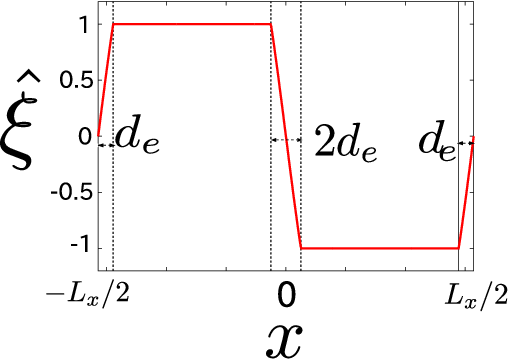
Let us a priori choose the piecewise-linear test function shown in FIG. 4. By substituting this function into (9) and (10), we can make $W^{(2)}$ negative and keep $I^{(2)}$ finite as follows: $I^{(2)}\simeq 4/d_{e}k^{2}$, $W^{(2)}\simeq-2\left(1/3+9e^{-2}\right)d_{e}B_{y0}^{\prime 2}$, where $B_{y0}^{\prime}=\alpha^{2}\psi_{0}$ and we have extracted only the leading-order term. The linear growth rate is therefore estimated as

where $\tau_{0}^{-1}=d_{e}kB_{y0}^{\prime}$. This result agrees with the general dispersion relation derived by asymptotic matching [3, 4]. Of course, our analytical estimate of the growth rate depends on how good the chosen test function mimics the genuine eigenfunction. Nevertheless, the result predicted by the simple function in FIG. 4 shows a satisfactory agreement with the numerically calculated growth rate (see FIG. 4) in the small $k$ region corresponding to the ordering (4).

Next, we consider the nonlinear phase of the linear instability discussed above. We remark in advance that a higher-order perturbation analysis of the Lagrangian (i.e., weakly nonlinear analysis) [17] will not be successful. Such a perturbation expansion will fail to converge when the displacement $\epsilon$ (or the island width) reaches the boundary layer width ($\sim d_{e}$), since the eigenfunction has a steep gradient $\hat{\xi}^{\prime}\sim\hat{\xi}/d_{e}$ inside the boundary layers (see FIG. 4). The naive perturbation analysis is, therefore, only valid for $0\leq\epsilon\ll d_{e}$, while $\epsilon$ actually exceeds $d_{e}$ without saturation as in FIG. 2.

To avoid difficulties of a rigorous fully-nonlinear analysis, we again take advantage of the variational approach. Namely, we devise a trial fluid motion (parameterized by the amplitude $\epsilon$) that tends to decrease the potential energy $W$ as much as possible. When such a motion is substituted into the Lagrangian (5), it is expected to be nonlinearly unstable.

Owing to the symmetry of the mode pattern, it is enough to discuss the boundary layer at $x=0$ and, moreover, focus on only the 1st quadrant, $0<x$ and $0<y<L_{y}/2$. In a heuristic way based on the simulation result, we consider a displacement map $\bm{G}_{\epsilon}:(x_{0},y_{0})\mapsto(x,y)$ where the displacement in the $x$ direction is prescribed by

The regions (i)-(iii) are indicated in FIG. 5(left) and we furthermore define $g_{\epsilon}$ as

As illustrated in FIG. 5(right), this displacement map deforms the contours of $\psi_{e}$ into a Y-shape. From this deformation we find that the potential energy decreases as follows:

in a nonlinear regime $d_{e}\ll\epsilon\ll L_{x}$. To obtain the estimate (14) that is likely close to the steepest descent, we have technically chosen the map (12) based on the following observations:

• •

  Around the X points, the flux $\psi_{e}$ of the red regions of FIG. 5(left) is squeezed into the boundary layers in FIG. 5(right). On the other hand, the flux is expanded around the O points and the areas of the blue regions of FIG. 5(left) are almost doubled in FIG. 5(right). Since $\psi_{e}\simeq\psi$ except for the boundary layers, both deformations are found to decrease magnetic energy $(1/2)\int|\nabla\psi|^{2}d^{2}x$ as $\epsilon^{3}$ when $d_{e}\ll\epsilon\ll L_{x}$.

• •

  As is also shown in Ref. [6], a strong current spike develops inside the boundary layers [i.e., the red regions in FIG. 5(right)] in the form of $J\simeq\hat{\epsilon}B_{y0}^{\prime}\log|x/d_{e}|$ for $\hat{\epsilon}=\epsilon/d_{e}\gg 1$, which increases the current energy $(1/2)\int d_{e}^{2}J^{2}d^{2}x$ (where $J=-\nabla^{2}\psi$). However, this logarithmic singularity is square-integrable and the current energy change is, at most, of the second order $O(\hat{\epsilon}^{2})$ in (14).

• •

  Only in the intermediate region (ii) located between the X and O points, does the potential energy tend to increase. But, we can omit the detailed analysis of this region by taking its width $l$ to be sufficiently small: $l\ll L_{y}$. We are allowed to use this approximation as far as the kink-tearing ordering (4) is concerned, in which $L_{y}$ is the longest length scale.

By introducing time-dependence in $\epsilon(t)$, we also need to calculate the kinetic energy, which eventually results in

where $\hat{t}=t/\tau_{0}$. Therefore the Lagrangian (5) reduces to

where $U(\hat{\epsilon})=-(3/\pi^{2}\log 2)\hat{\epsilon}^{3}+O(\hat{\epsilon}^{2})=-0.439\hat{\epsilon}^{3}+O(\hat{\epsilon}^{2})$. In the linear regime ($\hat{\epsilon}\ll 1$), we have already shown that the potential energy decreases as $U(\hat{\epsilon})=-0.776\hat{\epsilon}^{2}$. The steeper descent where $U(\hat{\epsilon})=-0.439\hat{\epsilon}^{3}$ in the nonlinear regime ($\hat{\epsilon}\gg 1$) indicates an explosive growth of $\epsilon$ during a finite time $\sim\tau_{0}$.

We remark that the nonlinear force $F(\hat{\epsilon})=-U^{\prime}(\hat{\epsilon})\sim O(\hat{\epsilon^{2}})$ obtained here is different from $F(\hat{\epsilon})\sim O(\hat{\epsilon}^{4})$ in the earlier work [6]. While the similar fluid motion around the X and O points is considered in Ref. [6], they directly integrate the vorticity equation (1) over the quadrant $[0,L_{x}/2]\times[0,L_{y}/2]$ and arrive at an equation of motion $d^{2}\hat{\epsilon}/d\hat{t}^{2}=F(\hat{\epsilon})\sim O(\hat{\epsilon}^{4})$. However, unless the assumed trial motion happens to be an exact solution, their treatment may lead to a wrong equation of motion that does not satisfy energy conservation.

In direct numerical simulation, we have calculated the potential energy $U(\hat{\epsilon})$ [or, equivalently, the kinetic energy $(d\hat{\epsilon}/d\hat{t})^{2}$] as a function of $\hat{\epsilon}$. As shown in FIG. 6, the decrease of $U(\hat{\epsilon})$ agrees with our scaling and does not support the scaling $U\sim-\hat{\epsilon}^{5}$ of Ref. [6].

In this work, we have analytically elucidated the acceleration mechanism for collisionless reconnection driven by electron inertia. Let us interpret our result for tokamak parameters. For the $m=1$ kink-tearing mode in tokamaks, $\tau_{0}^{-1}=d_{e}kB_{y0}^{\prime}$ corresponds to $\tau_{0}^{-1}=d_{e}q^{\prime}_{1}\omega_{A0}$, where $q^{\prime}_{1}$ is the derivative of the safety factor $q$ at the $q=1$ surface and $\omega_{A0}$ is the toroidal Alfvén frequency at the magnetic axis. In order for the reconnection to be collisionless, the time scale $\tau_{0}$ should be shorter than the electron-ion collision time $\tau_{e}=\mu_{0}d_{e}^{2}/\eta$, where $\eta$ is the resistivity (at the $q=1$ surface) and $\mu_{0}$ is magnetic permeability [13]. For sample parameters, $\omega_{A0}=6.4\times 10^{6}{\rm s^{-1}}$, $T_{e}=6{\rm keV}$, $n=3.5\times 10^{19}{\rm m^{-3}}$ and $q_{1}^{\prime}=2.0{\rm m^{-1}}$ of TFTR [18], we obtain $\tau_{0}=90{\rm\mu s}$ and $\tau_{e}=270{\rm\mu s}$. Although the ratio $\tau_{0}/\tau_{e}$ can drastically change in proportion to $T_{e}^{-3/2}n^{2}$, these two time scales are not so separated but possibly similar in tokamak plasmas.

Nevertheless, the time scale of explosion $\tau_{0}$ predicted in this work is comparable to the experimental sawtooth collapse times $\sim 100{\rm\mu s}$ [18]. Note, inclusion of resistivity into Ohm’s law (2) causes an additional decrease of the potential energy, one that would not prevent the release of free energy by inertia. In fact, our simulations exhibit nonlinear acceleration even with resistivity satisfying $\tau_{0}/\tau_{e}<1$. While the model used here is very simple, our result can be a central mechanism for sawtooth collapse.

As might be expected, this explosive growth will be decelerated eventually before $\epsilon$ reaches the equilibrium scale size $L_{x}$ (when the free energy starts to be exhausted). In tokamaks, we infer that the state of minimum potential energy is similar to the final state of Kadomtsev’s model [1]. But, if dissipation were sufficiently small, it would also corresponds to the state of maximum kinetic energy, where a strong convective flow remains. As shown in numerical simulations [14, 15], such a residual flow will cause a secondary reconnection and restore a magnetic field similar to the original equilibrium.

We expect further applications of this variational approach to be fruitful for predicting strongly nonlinear and nonequilibrium dynamics of sawtooth collapses that other analytical methods fail to clarify. In addition to the theoretical estimation of the fast collapse time, a legitimate derivation of a partial reconnection model (as well as associated loss of stored energy $\delta W$) would be made possible by extending the present analysis to more realistic two-fluid equations in tokamak geometry.

References

- [1] KADOMTSEV, B. B., Sov. J. Plasma Phys. 1 389 (1975).
- [2] WAELBROECK, F. L. Phys. Fluids B 1 2372 (1989).
- [3] BASU, B. and COPPI, B., Phys. Fluids 24, 465 (1981).
- [4] PORCELLI, P., Phys. Rev. Lett. 66, 425 (1991).
- [5] AYDEMIR, A. Y., Phys. Fluids B 4 2469 (1992).
- [6] OTTAVIANI, M. and PORCELLI, F., Phys. Rev. Lett. 71, 3802 (1993).
- [7] MATSUMOTO. T. et al., Phys. Plasmas 12, 092505 (2005).
- [8] RUTHERFORD, P. H., Phys. Fluids 16 1903 (1973).
- [9] CAFARO, E., et al., Phys. Rev. Lett. 80 4430 (1998).
- [10] GRASSO, D., et al., Plasma Phys. Control. Fusion 41 1497 (1999).
- [11] TASSI, E., et al., Nucl. Fusion 50 034007 (2010).
- [12] BERNSTEIN, I. B. et al., Proc. Roy. Soc. London A244, 17 (1958).
- [13] WESSON, J. A., Nucl. Fusion 30 2545 (1990).
- [14] BISKAMP, D. and DRAKE, J. F., Phys. Rev. Lett. 73, 971 (1994).
- [15] NAITOU, H. et al., Phys. Plasmas 2, 4257 (1995).
- [16] NEWCOMB, W. A., Nucl. Fusion Suppl. Pt. 2, 451 (1962).
- [17] HIROTA, M., J. Plasma Phys., 77, 589 (2011).
- [18] YAMADA, M. et al., Phys. Plasmas, 1, 3269 (1994).