-ray DBSCAN: a clustering algorithm applied to Fermi-LAT -ray data.
Abstract
Context. The Density Based Spatial Clustering of Applications with Noise (DBSCAN) is a topometric algorithm used to cluster spatial data that are affected by background noise. For the first time, we propose the use of this method for the detection of sources in -ray astrophysical images obtained from the Fermi-LAT data, where each point corresponds to the arrival direction of a photon.
Aims. We investigate the detection performance of the -ray DBSCAN in terms of detection efficiency and rejection of spurious clusters.
Methods. We use a parametric approach, exploring a large volume of the -ray DBSCAN parameter space. By means of simulated data we statistically characterize the -ray DBSCAN, finding signatures that differentiate purely random fields, from fields with sources. We define a significance level for the detected clusters, and we successfully test this significance with our simulated data. We apply the method to real data, and we find an excellent agreement with the results obtained with simulated data.
Results. We find that the -ray DBSCAN can be successfully used in the detection of clusters in -ray data. The significance returned by our algorithm is strongly correlated with that provided by the Maximum Likelihood analysis with standard Fermi-LAT software, and can be used to safely remove spurious clusters. The positional accuracy of the reconstructed cluster centroid compares to that returned by standard Maximum Likelihood analysis, allowing to look for astrophysical counterparts in narrow regions, minimizing the chance probability in the counterpart association.
Conclusions. We find that -ray DBSCAN is a powerful tool in the detection of clusters in -ray data, this method can be used both to look for point-like sources, and extended sources, and can be potentially applied to any astrophysical field related with detection of clusters in data. In a companion paper we will present the application of the -ray DBSCAN to the full Fermi-LAT sky, discussing the potentiality in the discovery of new sources.
Key Words.
Gamma rays: general – Methods: statistical – Methods: data analysis1 Introduction
Modern -ray telescopes operating at energies above the MeV window, provide event-resolved observational data. Each event (after the reconstruction process) is typically described by a tuple (i.e. an ordered list of elements) storing sky coordinates, arrival time, and energy. Detection of discrete sources (either point-like or extended) is performed using various methods. Given the discrete topological nature of -ray images, methods based on cluster search, like the Minimum Spanning Three (MST) (Campana et al., 2007; Campana et al., 2012) have successfully been used. One of the main advantages of topometric methods, compared to methods using the spatial binning, is to minimize the impact of the poor energy-dependent Point Spread Function (PSF), typical of -ray telescopes, preserving the spatial information of each event. Moreover, these methods are able to detect sources compounded by a small amount of events, but they need to be fine tuned to take into account properly the background. The problem of background rejection is the most penalizing feature of topometric methods, for this reason in this paper, for the first time, we present a method based on the DBSCAN algorithm (Ester et al., 1996). The DBSCAN is a topometric algorithm used to cluster spatial data that are affected by background noise. Compared to other topometric methods, it has the advantage to embed inside the algorithm itself the discrimination between signal (cluster) and background (noise), according to the local density of events within a typical scanning brush i.e. within a given scanning area.
The aim of the present paper is to show the potentialities of the method, and its statistical characterization when applied to astrophysical -ray data. We apply this method to the detection of point-like sources in the Fermi-LAT data. We explore a large volume of the -ray DBSCAN parameter space, by means of simulated data, and we provide a statistical characterization the -ray DBSCAN, finding signatures that differentiate purely random fields, from fields with sources. We define a significance level for the detected clusters, and we successfully test this significance with our simulated data. We apply the method to real Fermi-LAT -ray data, and we find an excellent agreement with the results obtained with simulated data.
In a companion paper (Tramacere, 2012), we will apply the method to the Fermi-LAT sky, investigating specific issues related to the Fermi-LAT response functions, showing the potentiality for the discovery of new sources, in particular of small clusters located at high galactic latitude, or clusters on the galactic plane, affected by a strong background.
The paper is organized as follows. In Sec. 2 we describe the logic of the DBSCAN method, and we present the algorithm implemented to analyse -ray data, the -ray DBSCAN. In Sec. 3 we discuss some caveats regarding the application of the -ray DBSCAN algorithm to -ray data. In Sec. 4 we study the statistical properties of the -ray DBSCAN detection, using a simulated test field with only noise, and five simulated test fields with noise plus point-like sources. In Sec. 5 we evaluate the detection performance of the method in terms of positional accuracy, cluster reconstruction, and rejection of spurious clusters. In Sec. 6 we investigate the significance of the clusters, and describe our algorithmic implementation. In Section 7 we finally use our method with real Fermi-LAT data, investigating the detection performance, and comparing the -ray DBSCAN clusters significance, to that returned by the Maximum Likelihood method with standard Fermi-LAT software 11 1 http://fermi.gsfc.nasa.gov/ssc/data/analysis/scitools/overview.html. In Section 8, we present our conclusions, and we discuss future developments and applications.
 |
2 The -ray DBSCAN algorithm
The DBSCAN (Ester et al., 1996) is a topometric algorithm used to cluster spatial data that are affected by background noise. Some modifications have been developed to adapt the original DBSCAN algorithm to our study. Our algorithm is mainly built upon the following criteria:
- 1.
given a list of photons , where each element is a tuple storing positional sky coordinates, let be the angular distance between two photons and .
- 2.
We iterate over the full photon list . A seed cluster is built when a minimum number of photons is enclosed within a circle of radius centered on
- 3.
For each photon , we build the photon list by collecting all the photons respecting the condition: , and .
- 4.
For each photon , if the number of photons enclosed within a circle of radius centered on is and , then will be attached to the final photon list of the cluster without a recursive search for further neighbours, these points are defined density-reachable.
- 5.
For each photon , if the number of photons enclosed within a circle of radius centered on is and , is attached to the , and and step 3 is repeated recursively.
- 6.
When both conditions at step 4 and 5 are false, the cluster is built by joining the density-reachable events to those in the and in the lists.
- 7.
The process starts again from step 1 searching for new clusters, skipping all the events already flagged as noise or clusters, until all the events in are flagged as cluster, or noise, or density-reachable, events.
- 8.
At the end of the process the full photon list will be partitioned as follows:
(1)
In this way high densely populated areas are classified as clusters (sources), conversely low densely populated areas are classified as noise (background). The recursive call of step 3, is not implemented in the original DBSCAN algorithm, and represents a novelty. This new feature, allows to reconstruct clusters with a size significantly larger than the radius, making rare the possibility to fragment a single clusters in small satellite clusters. Moreover, allows the possibility to reconstruct extended structures, in particular extended sources, or filamentary structures in the background.
After the clustering process, each photon in will be described by a tuple, storing: the photon position (both in galactic and celestial coordinates), the photon class type (noise or cluster), and the ID of the cluster the photon belongs to. Each cluster , will be described by a tuple storing the position of the centroid with his positional error, the ellipse of the cluster containment, the cluster effective radius (), and number of photons in the cluster (). The ellipse of the cluster containment, is defined by major and minor semi-axis ( and , respectively), and the inclination angle () of the major semi-axis w.r.t. the latitudinal coordinate. ( or ). To evaluate the ellipse axis we use the Principal Component Analysis method (PCA) (Jolliffe, 1986). This method uses the eigenvalue decomposition of the covariance matrix of the the two position arrays , and . By definition, the square root of the first eigenvalue will correspond to , and the second to . The axes represent the two orthogonal directions of maximum variance of the cluster. The effective radius is defined as . To find the centroid of the cluster and its uncertainty, we use a weighted average of the position of each photon in , as follows:
- •
we define the first order centroid () as the average of the position of each cluster photon: .
- •
We define the weight array, according to the distance between and : .
- •
The cluster centroid will result from average of the position of each cluster point weighted by .
- •
The centroid position uncertainty () is determined by propagating the error on the weighted average of . We have numerically verified that corresponds to a positional uncertainty.
3 Caveat on the application to -ray data
The application of clustering methods, such as the -ray DBSCAN, leads to deal with practical difficulties, related mostly to the instrument PSF, and to gradient and/or structures in the background. In order to deal with these issues, without biasing the detection results, it’s recommended to apply some criteria that we discuss in the following.
As first, we comment on the PSF impact. The PSF imposes a limit on the capability
of an instrument to resolve sources separated by a distance smaller then the PSF
size. Sources with sizes below the PSF classified as point-like, otherwise are classified as extended. A further complication is that the PSF
often depends on the energy; in the case of Fermi-LAT, the containment angle of the
reconstructed incoming photon direction, for normal incidence photons, has a typical
size of a couple of degrees at 100 MeV (Fermi-LAT Collaboration, 2012), and scales down to few tenths of
degree above the GeV energies
22
2
http://www.slac.stanford.edu/exp/glast/groups/canda/
lat_Performance.html.
The size of the PSF is strongly connected to the size of the
-ray DBSCAN scanning brush. Indeed, if is much smaller than the PSF size, it
might occur the risk to loose clusters characterized by small , or to fragment a
cluster with large in smaller fake satellite clusters.
We stress that the formation of satellite clusters is a very rare event,
thanks to our recursive DBSCAN implementation, that is explained in Sec. 2.
On the contrary, if is much larger w.r.t the PSF, it is likely to build extended
clusters contaminated by the background, or by close sources.
A careful and self-consistent analysis of the effects of the energy dependence
of the PSF, and in general of issues related to the Fermi-LAT response function,
is beyond the scope of this paper, where we focus mostly on a statistical
characterization of the method.
These subjects will be investigated in the companion paper (Tramacere, 2012).
A second relevant issue, is the inhomogeneity of the background, that affects both the choice of and . If the background is homogeneous over the entire field, the optimal choice of a single pair of values of and , guarantees a safe rejection of the background. Indeed, values of and , such that the average density of photons within is significantly larger the the average density of the background photons, make rare the chance to grow a cluster from a background fluctuation. Unfortunately, the -ray sky shows strong gradients of background, in particular at low galactic latitudes. To solve this issue, one could think to adapt the value of and according to a local value of the background photon density. Since has a strong constraint imposed by the PSF, one should tune mostly the value of . The drawback is that as we increase the value of to compensate for the background, we decrease the capability to detect cluster with small . To overcome this difficulty, we adopt an alternative solution. We use a unique pair of values of and , for each field, where is mostly constrained by the PSF, and , by the field average background, ad we take into account the background inhomogeneities by defining a significance level of the cluster, according to the signal to noise ratio (Li & Ma, 1983), evaluated from the local background. This is explained in detail in Section 6. The capability to reject clusters according to a low significance level, allows to relax the constrain on and , increasing the number of clusters detected, hence increasing the detection ratio, and at the same time allows to reject spurious sources, due to the significance threshold. Anyhow, to avoid that the background is so high, that the fluctuations in the background events, can lead to densities comparable to those of weak sources, it’s recommended to apply a cut in energy, to make this possibility rare. In order to optimize the ratio between background and clusters events, in the following we use a threshold energy of 3 GeV, that mitigates the possible bias due to the background fluctuations.
4 Statistical properties of the -ray DBSCAN clusters
4.1 The test fields
In this section we study the statistical properties of the clusters, looking for signatures that characterize random Poissonian fields, and fields with point-like sources. To accomplish this task we compare results obtained for a test field with only noise (random test field), and the five test fields with noise plus point-like sources (sky test fields 1-5).
As sky test fields we use the same fields used in the Campana et al. (2012). Each of these five sky fields covers a broad sky region, with a galactic longitude extension of , and a galactic latitude extension of . The -ray background has been simulated using the standard gtobssim 33 3 http://fermi.gsfc.nasa.gov/ssc/data/analysis/scitools/help/gtobssim. txt tool, developed by the Fermi-LAT collaboration, simulating both the Galactic and isotropic components for a 2-year long period, using a threshold energy of 3 GeV, for a total amount of 9322 photons. To this photon list we added 70 simulated sources: for each source, the number of photons was chosen from a probability distribution given by a power-law, with exponent 2, from a minimum value of 4 up to 40 photons, joined to a constant tail up to 240 photons. The number of the sources is similar to that reported in the Fermi-LAT Second Source Catalog (Nolan et al., 2012, 2FGL hereafter), in the same region of the sky. The source events are spatially distributed with a bivariate Gaussian probability density function (PDF) with deg., centered at the source location. Five simulated test fields have been generated, adding the simulated sources to the diffuse background. The only difference in the five realizations is the source location, randomly chosen to have different brightness contrast between sources and the background. The random test field covers the same area of the sky test fields, and a number of events equal to the sky test field-1 (background and sources), for a total amount of 11044 events.
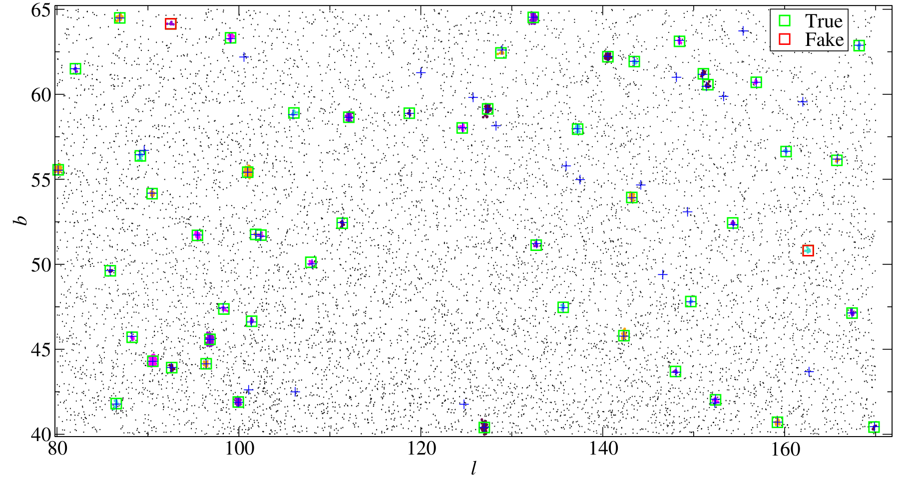
In Fig. 1 we show the photon map for the sky test field 1, and the result of the -ray DBSCAN detection for and deg. We detect 51 true clusters, and only 2 fake ones. A cluster is defined true, if the position of the simulated source falls within a circle centered on the cluster centroid, with a radius equal to . We call fake, the remaining clusters. In Fig. 2, we show a close-up of two true clusters. The black ellipses correspond to the ellipses of the positional error, and the purple and orange thick points represent the cluster points, while the black thick dots represent the background.
4.2 Test strategy
We want to investigate the statistical properties of the -ray DBSCAN clusters, in particular signatures that distinguish purely random fields from fields with point-like sources, and their dependence on and . To investigate systematically a broad volume of the parameter space, we use a parametric approach. We set the range of in [0.10.50] deg. with a step of 0.01 deg., and the range of in [215], with a step of 1. The total amount of detection trials for each test field is 574. We collect the statistics of the trials, and we investigate the distribution of and , and their connection with and , respectively.
4.3 Statistics of and connection with
We start by investigating the distribution of the values, in the case of the random, and of the sky test field-1. The distribution for the detections collected over the full - parameter space (top left panel of Fig. 3), shows a symmetric shape well fitted by a Gaussian distribution (log-normal w.r.t. ), with the mean value of (corresponding to deg) and a dispersion of 0.23. The log-normal distribution provides a reasonable description of the empirical distributions also for individual pairs of (,) values. An example is given in panel c of Fig. 3, for the case , deg., where the best fit values are , and 0.16. We now investigate the empirical distribution of for fields with point-like sources. In the right panel of Fig. 3, we show the case of the sky test field-1. The distributions of are still described by a by a normal. In the case of fake clusters (red dashed line), the best fit values of the mean () and of the dispersion ( 0.24), are very similar to those found in the case of the random test field. On the contrary, the true cluster distribution (blue hatched histogram) is peaking around the value of deg, corresponding to . deg., very close to the value of the dispersion deg., used to simulate the sources. Since the simulation parameter reproduces the effect of the instrumental PSF, we observe that for non-random fields, the typical size of the reconstructed clusters is constrained by the PSF, suggesting the empirical rule to set the value of of the order of the PSF size.
To investigate more accurately the connection between and the PSF, we analyse the statistical properties of the quantity as a function of . For each value of , we determine the median, and the two-sided 1- confidence level (CL) interval around the median, of the distributions. In the left panel of Fig. 4 we plot the median (blue solid circles) and 1- CL region, as a function of , for the random field. We note that the trend is slightly increasing with , and that the 1- CL region is consistent with the case , but the upper boundary shows a systematic increase, compared to the lower boundary, for deg. The trend for the case of the true clusters in sky test field 1 (right panel Fig.4), shows a different behaviour. The median of (red solid circles) is slightly decreasing with , showing that, for true clusters, is not sensitive to the size of , being mostly constrained by the simulated PSF size. As expected, for the case of fake clusters (blue dashed line), the trend is almost identical to that of the clusters in the random field.
4.4 Statistics of and connection with
We now investigate the statistics of the distribution of the number of photons per cluster. In the case of random fields, we expect that the number of photons in a cluster attends a Poisson distribution. Indeed, for a generic two-dimensional Poisson process, the probability to observe a number of events () enclosed by a surface is given by:
| (2) |
where is the average spatial density. Translating in terms of , we can rewrite:
| (3) |
from which follows that, given the value of and , the probability to find a cluster as function of and will be given by
| (4) |
namely the Poissonian survival function. Anyhow, due to the logic of the DBSCAN clustering process, the Poisson statistics can’t be extended from to , for any value of . Indeed, a cluster is not a simple collection of points enclosed within a surface , this holds only within the -sized circle, namely the seed of the cluster (). If we consider the annulus defined between and the cluster radius , not all the points in the annulus will be cluster member, but only those that are at least density reachable. This implies that we expect a deviation from the Poisson statistics, when is significantly larger than , i.e. 0.3 deg. (according to the analysis presented in the previous section). This expected deviation from the Poissonian statistics, is confirmed by the plots in the left panels of Fig. 5. In panel a we show the distribution of for the case and deg. We note that the Poisson distribution (Eq. 3) gives a reasonable description of the empirical distribution. On the contrary, for the case of deg. (panel b), we observe that the Poisson distribution shows larger deviations, in particular for . When we take into account the distribution for the full parameter space (panel c), we note the Possonian distribution is failing in providing a reasonable description of the empirical distribution, whilst a log-normal one gives a good fit.

The log-normal trend of is consistent with the log-normal trend of the distribution of . Since the number of photons in a cluster will be approximatively , we can write the PDF of :
| (5) |
To evaluate the distribution of we can use the standard theory of the transformation of Random Variables (RV) (Papoulis, 1965). It can be easily proved that, given a RV having a log-normal distribution,
| (6) |
the RV , will follow a log-normal distribution given by:
| (7) |
Indeed, our distribution, for the random field (panel d, Fig. 5), is fitted by a log-normal distribution peaking at deg2. Hence, according to Eq. 5 we expect that also will follow a log-normal distribution, when is not ruled by a Poissonian statistics.
We verify, that the same statistical trends, describe the real sky fields. The panels e and f in Fig. 5, show the statistical distribution of for the sky test field 1 case. In agreement with the analysis concerning the random test field, we see that the fake clusters ( deg., panel e in Fig. 5), are described by a Possonian statistic, whilst, the true clusters (panel f in Fig. 5), are better described by a log-normal distribution (red dashed line), compared to a Poissonian one (solid black line). We also observe that the log-normal law, describes reasonably the empirical distribution, only for values of , whilst shows significant deviation in the tail, consistent with the statistics of our simulated sources population.
To complete this statistical characterization, we investigate the distribution of the number of detected clusters, as a function of the threshold . According to Eq. 4, we expect that the number of detected cluster, for a random field, follows a Poisson survival distribution. The plot a of Fig. 6 confirms our hypothesis, indeed the Poisson survival function provides a reasonable description of the empirical distribution. The same holds for the case of fake clusters of the sky test field 1 (plot c Fig. 6). On the contrary, in the case of true clusters (panel d Fig. 6), the Poisson survival distribution is not able to reproduce the observed trend, consistently with the non-poissonian statistic of the simulated clusters . The panels b and e of Fig. 6, show the CL region for the , as a function of . We note, that both in the case of random and sky field true clusters, the lower boundary of the region is constrained by the equation , that is consistent with the -ray DBSCAN logic. On the contrary, the upper boundary shows a different behaviour. In the case of the random field, the upper boundary deviates from the lower boundary compatibly with the fluctuations of the events around the circle, and ranges from about 8 to about 16. On the contrary, in the case of sky field true the upper boundary is constrained by the statistics of the number of events in the simulated sources, and rages from about 60 to 100.
5 Testing the detection performance with simulated -ray data
In this section we investigate the detection performance of the -ray DBSCAN. As first point, we study the dependency of the detection efficiency on and , and their impact on the spurious ratio, and on the detection efficiency. Then, we investigate the capability of the algorithm to reconstruct the simulated clusters, and the positional accuracy of the reconstructed centroids. We test the detection performance of the -ray DBSCAN using as benchmark the five sky test fields used in the previous section, and exploring the same parameter space.
5.1 Detection efficiency and spurious ratio as a function of and
To investigate the detection performance of the -ray DBSCAN, we run, for each of the five sky test fields, and for each pair of values ,, a -ray DBSCAN detection. For each detection run, we build a cluster catalog. Starting from the cluster catalog, we build the corresponding candidate catalog. The candidate catalog is a list of sources built by taking into account two possible biases, the confusion, and the multiple association, in detail:
- •
a cluster is defined true, i.e. with a possible counterpart, if the position of the simulated source falls within a circle centered on the cluster centroid, with a radius equal to .
- •
Two or more true clusters are defined confused, if they have the same counterpart
- •
A true cluster has a multiple association, if has more than one counterpart.
We stress that, the number of confused clusters is negligible, indeed the average number of confused clusters per run is about 0.08, and no confused clusters are found for , and that the average number of multiple associations per run is about 0.2.
The final candidate catalog will count a number of candidate sources , each identified by a unique . The number of spurious sources will be . In order to to characterize the performance, we define the following parameters:
- •
the detection efficiency:
(8) where is the number of simulated sources with a number of simulated events larger than
- •
the true detection ratio
- •
the spurious detection ratio
- •
the overall detection quality factor (), that takes into account the tradeoff between and , defined as:
(9)
The parameter shows the fraction of simulated clusters, above the threshold , detected by the method, net of the fake ones. Hence, does not provide an indication of the spurious contamination. For this reason we have introduced the parameter, which rescale the according to the ratio between fake clusters, and found clusters . We remind that, according to the definition in Eq. 8, it’s possible to obtain values of . Assume to have a simulated cluster such that, for a given and , the corresponding seed cluster has a size . In the case of no background events within the circle of radius , this cluster will be rejected. If we have one or more background events contained within the circle of radius , i.e. , the cluster will be detected. For this reason, in such a case, we report a value of . The same applies to .
In Fig. 7 we summarize the detection runs for the case of sky test field 1, for the full parameters space with . The panel a shows the isolevel map of the fake clusters detection ratio. The gradient in the isolevel map is quite sharp, and roughly half of the parameter space shows no fake clusters (white isolevel line). To have a better understanding of the impact of fake clusters, it’s interesting to compare the isolevel map to the isolevel map (panel b Fig. 7). Also in this case the map shows a sharp gradient, and the region with overlaps the region. These two maps, clearly show the region of the parameter space where the algorithm has the best performance, but the and ratios do not provide information on the ratio between the number of true detected clusters and the number of simulated clusters. At this regard more information are provided by the isolevel map (panel c, Fig. 7). To focus on the "effective" volume of the parameter space, we hide by a white area the region where . We note that the isolevel lines and the isomap lines in the maximum gradient area show a positive correlation between and , meaning that an increased value of , requires an increased value of , to have better background rejection. To evaluate better the trade-off between and , we plot in the panel d of Fig. 7, the isolevel map of . This plot shows that the area corresponding to , is consistent with that found in the case of . In Tab. 1 we report the values obtained for all the five sky fields, for detections with a number of fake sources 6. We note that the average values of true clusters ranges between 44 and 51, with the fake ones ranging between 1 and 3, and an average between 0.96 and 1.0. This is a very promising result.
5.2 Cluster reconstruction, and positional accuracy
The positional accuracy of the topometric methods, is probably the most important feature of this class of algorithms. In Sec. 2, we have described our weighting method to reconstruct the centroid of the cluster.
The panel a of Fig. 8 shows by red solid boxes the mean positional error of the clusters centroid and the standard deviation (vertical error bar) vs. , for the true clusters of the sky test field 1 with deg. The clusters are binned in , with the bin width indicated by the horizontal error bar. As expected, the uncertainty on the reconstructed cluster centroid is (solid red line). The solid black circles represent the corresponding trend for the separation between the simulated cluster position and the reconstructed cluster centroid. For , the separation is below . In the panel b of Fig. 8 we plot the histogram of the distribution of the angular separation between the position of the simulated source, and the position of the cluster centroid. For the three cases of deg., deg., and deg., the positional error is below the , for the of the sample.
| True | Fake | ||||||
| sky field 1 | 44/70 | 47 | 1 | 6 | 0.19 | 1.00 | 1.00 |
| 38/70 | 48 | 2 | 8 | 0.27 | 1.00 | 1.00 | |
| 53/70 | 50 | 3 | 5 | 0.17 | 0.89 | 0.84 | |
| 62/70 | 51 | 5 | 4 | 0.14 | 0.74 | 0.68 | |
| 53/70 | 53 | 6 | 5 | 0.18 | 0.89 | 0.80 | |
| average | 50.00 | 49.80 | 3.40 | 5.60 | 0.19 | 0.90 | 0.86 |
| sky field 2 | 62/70 | 47 | 0 | 4 | 0.11 | 0.76 | 0.76 |
| 44/70 | 49 | 2 | 6 | 0.20 | 1.00 | 1.00 | |
| 53/70 | 51 | 3 | 5 | 0.17 | 0.91 | 0.86 | |
| 62/70 | 52 | 6 | 4 | 0.14 | 0.74 | 0.67 | |
| average | 55.25 | 49.75 | 2.75 | 4.75 | 0.15 | 0.85 | 0.82 |
| sky field 3 | 41/70 | 42 | 0 | 7 | 0.22 | 1.00 | 1.00 |
| 44/70 | 45 | 2 | 6 | 0.20 | 0.98 | 0.94 | |
| 53/70 | 46 | 3 | 5 | 0.16 | 0.81 | 0.76 | |
| 62/70 | 48 | 5 | 4 | 0.14 | 0.69 | 0.63 | |
| 62/70 | 50 | 6 | 4 | 0.15 | 0.71 | 0.63 | |
| average | 52.40 | 46.20 | 3.20 | 5.20 | 0.17 | 0.84 | 0.79 |
| sky field 4 | 53/70 | 47 | 1 | 5 | 0.16 | 0.87 | 0.85 |
| 53/70 | 50 | 5 | 5 | 0.18 | 0.85 | 0.77 | |
| 62/70 | 52 | 6 | 4 | 0.14 | 0.74 | 0.67 | |
| average | 56.00 | 49.67 | 4.00 | 4.67 | 0.16 | 0.82 | 0.76 |
| sky field 5 | 44/70 | 47 | 1 | 6 | 0.19 | 1.00 | 1.00 |
| 44/70 | 50 | 2 | 6 | 0.20 | 1.00 | 1.00 | |
| 44/70 | 53 | 3 | 6 | 0.21 | 1.00 | 1.00 | |
| 44/70 | 55 | 5 | 6 | 0.22 | 1.00 | 1.00 | |
| average | 44.00 | 51.25 | 2.75 | 6.00 | 0.20 | 1.00 | 1.00 |
Besides positional accuracy, is also important to understand the capability of the -ray DBSCAN to reconstruct the simulated cluster in terms of number of photons. Indeed, this information gives an idea of the average number of background photons contaminating the reconstructed cluster. In the top left panel of Fig. 9, we show the scatter plot of vs. the number of simulated events ( sim.). The solid points represent the average value of , for a given value of sim., and the error bar, corresponds to the standard deviation. The solid green line represents the case sim., and the dashed upper and lower lines, represent sim., respectively. Both for the cases of deg., and deg., the scatter is bounded by the dashed lines, showing that the largest excess in the is about 10 photons, independently of sim. We note, that in the case of deg., the number of reconstructed photons, systematically underestimates the simulated number, whilst, the deg. case does not shows this bias. It’s possible to appreciate better this effect, in the bottom left panel of Fig. 9, where we show the fractional reconstruction error ( sim.)/ sim., vs. sim. The solid green line represent the case with 0 error, and the dashed lines represent the boundaries. The bias on in the case of deg., shows again the strong correlation between and the PSF radius. When is smaller then the (that in our simulations reproduces the PSF effect), the number of reconstructed events is systematically smaller than sim., on the contrary, when the radius matches the PSF radius size ( deg.), the bias disappears.
 |
6 Cluster significance, background inhomogeneities, and rejection of spurious clusters
Even though, we have identified the region of the - parameter space, where the detection efficiency is larger, and the probability to detect fake cluster is lower, in the application to real data, it’s mandatory to provide a significance level, expressing the probability of a cluster being not originated in a background fluctuation. We propose a method derived from the Li & Ma (1983) approach, based on the evaluation of the signal to noise (S/N) ratio. A significance method based on the S/N ratio fits well the the -ray DBSCAN implementation, because the algorithm directly provides a partition of the photon list in cluster and noise events. Hence, for each cluster we can evaluate easily the S/N ratio, knowing the exact nature of each event. The procedure to evaluate the significance is summarized by the following items:

- 1.
for each cluster, we define an annular region, with an inner radius , and an external radius .
- 2.
is set to an initial value of , and is adaptively increased with a step of , for a maximum of 10 trials, until at least the of the cluster events are enclosed within .
- 3.
is set to .
- 4.
We count all the cluster events and all the background events , enclosed within the circle with radius and centered on the cluster centroid.
- 5.
We determine the background level, rescaling the number of background events in , to a circle with radius .
- 6.
To evaluate possible gradients in the background, we select a region enough far from the cluster to sample properly the background level, and enough close to the cluster, to measure a ”local” background level. At this regard, we define the radius , and we evaluate the average background level () in a circle of radius , centered on each point in .
- 7.
If no background points are found in , we set .
- 8.
By comparing to , we evaluate the fraction of noise already resolved by the -ray DBSCAN, and we evaluate the effective background level , by correcting for .
- 9.
we evaluate the significance according to the Likelihood Ratio Test (LRT) method proposed by Li & Ma (1983):
(10)
Under the hypothesis that a cluster is due to a background fluctuation, the variable , is expected to follow a chi square distribution, with one degree of freedom (). In the left panel of Fig. 10, we plot the distribution of , for the fake clusters in the sky test field 1 (blue histogram), compared to a distribution. The empirical distribution, is well described by the expected distribution, proofing that the value of , can be used as the "significance" of the detected cluster. A very illustrative example of the power of in rejecting fake clusters, is given by the plot in the right panel in Fig 10, where we plot the ratio isolevel map, applying the selection . The fake ratio is 0 for the parameter space with deg. For 0.25 deg. 0.35 deg., there are fluctuations showing . Only for deg. and , the fake ratio shows a significant increase, but we stress that in this region of the parameter space, is more then double of the PSF size, hence this is a region of the parameter space that should not be used in the detection with real data.
7 Application to real Fermi-LAT data
The last step in our investigation of the -ray DBSCAN, is the application to real Fermi-LAT -ray data. We select the same region of the sky used for the simulated test field ( , and ), and we extract all the photons with energy GeV. The photons are collected for the same time span of the 2FGL catalog . We repeat the detection test performed in the case of simulated data (see Sec. 5 and Sec. 6), restricting the parameter space to , and deg.
 |
 |
 |
To properly understand the detection performance, we need to take into account that the 2FGL catalog has been built using photons with an energy threshold of 100 MeV, whilst we use a value of 3 GeV. A possibility is to select sources with a reported flux larger than zero, in the 3-10 GeV band flux column of the 2FGL. This flux-based selection, is not the best way to study the detection performance of the -ray DBSCAN , indeed the flux does not contain a unambiguous relation with the significance of the detection, for that energy threshold. A more reliable criterion is to select the sources according to the significance reported in the 2FGL. The 2FGL detection significance is given by the . The is the test statistic defined as , where is the likelihood of the data given the model with or without a source present at a given position on the sky (Nolan et al., 2012). We apply a selection according to , and we refer to the corresponding source list (counting 35 sources) as 2FGLTS>16.
An example of the application of the -ray DBSCAN to real Fermi-LAT data is given in Fig. 11, where we report an Aitoff projection in galactic coordinates of the analysed -ray sky region. The red crosses represent the 2FGL sources with in the 3-10 GeV band, and the green crosses represents those with . The purple boxes represent the -ray DBSCAN sources found for deg. For this choice of parameters, we find no fake sources, and we find all the sources with with , except only one, enclosed by the red circle, and positioned at the edge of the sky region, with a galactic latitude deg. In Tab. 2 we summarize the detection performance, for detections with a number of fake sources 4. We note that values of true clusters ranges between 35 and 34, out of the 35 present in the 2FGLTS>16. The fake ones range between 1 and 4, and we obtain an average detection efficiency of .
In Fig. 12 we compare the localization performance of the -ray DBSCAN algorithm with that returned by the likelihood analysis implemented in the Fermi Science Tools. For each source in our 2FGLTS>16 list, associated to one or more -ray DBSCAN clusters, we plot the the error on the position of the reconstructed cluster centroid and its standard deviation (represented by the error bar) vs. the 95 positional uncertainty reported in the 2FGL. We evaluate the 2FGL 95 positional uncertainty as , where and , are the semimajor and semiminor axes of the 95 confidence source location region, respectively. The dashed red line represents a linear best fit, with a slope of 0.99, and an intercept of 9.53, showing that the error on the position of the reconstructed cluster centroid, performed with a threshold of 3 GeV, is of the same order of the positional uncertainty reported in the 2FGL catalog, performed above 100 MeV.
To test the reliability of the significance to reject spurious sources, in Fig. 13 we plot the and , based on the 2FGLTS>16 catalog. The panels a and b, correspond to the case of no selection on . Both the and the trends are very similar to the case of the simulated sky. If we apply a significance cut of (panels c,d), we observe that the number of spurious ratio is 0.05 for almost half of the parameter space (region to the right of the purple line). The more severe cut of (panels d,e), removes all the fake clusters except two, for 0.15 deg. Only for 0.25 deg., the ratio shows a significant increase, ranging from 0.05 up to 0.1. In agreement with our analysis on simulated data, the region of the parameter space where is comparable to the PSF size, gives the better performance.
To have a further confirmation about the robustness of our significance, we plot in the right panel of Fig. 14, vs. . For each source in our 2FGLTS>16 list, associated to one or more -ray DBSCAN cluster, we plot the in the 3-10 GeV band, v.s. the average value of and its standard deviation (represented by the error bar). The average value of and its standard deviation are evaluated from the list of all the cluster associated to the same 2FGL source. The solid blue boxes represent the full , parameter space case, and the red solid circles represent the deg. case. The dashed black line represents a linear best fit. The slope of the linear fit is . The strong correlation in the scatter plots (, for both data sets), proves that our significance implementation is consistent with the reported in the 2FGL, and the slope of the linear fit suggests that .
| 2FGLTS>16 | True | Fake | |||||
|---|---|---|---|---|---|---|---|
| Fermi-sky | 35 | 34 | 0 | 8 | 0.21 | 0.97 | 0.97 |
| 35 | 34 | 1 | 7 | 0.20 | 0.94 | 0.92 | |
| 35 | 35 | 2 | 7 | 0.21 | 0.94 | 0.89 | |
| 35 | 35 | 4 | 6 | 0.19 | 0.89 | 0.79 | |
| average | 35 | 34.50 | 1.75 | 7.00 | 0.20 | 0.94 | 0.89 |
8 Conclusions
For the first time, we have used the DBSCAN for the detection of sources in -ray astrophysical images. We have implemented a new version of the DBSCAN, the -ray DBSCAN, that is optimized for the application to -ray astrophysical images, with relevant background noise. Our -ray DBSCAN, presents the novelty of recursive call of the DBSCAN algorithm, that allows an excellent reconstruction of the cluster, with an effective background rejection. We have tested the algorithm with a sample of simulated -ray Fermi-LAT fields, to give a statistical characterization of the method, and to benchmark the detection performance. The results, with the simulated -ray data, are summarized by the following items:
- •
The radius of -ray DBSCAN scanning brush , has a strong correlation with the instrumental PSF radius. We find that the typical size of the reconstructed true cluster is of the order of the simulated PSF size , and that the precision of the reconstructed centroid is of the order of .
- •
The number of reconstructed events is ruled by the Poissonian statistics in the random fields, and for the fake clusters. On the contrary, for true clusters, the statistics of , is ruled by that of the simulated sources.
- •
The fractional error on the reconstructed events number is of the order of for , and is negligible for larger values, with best performance obtained when .
- •
We have investigated the detection performance, for a wide range of the , parameter space, and we have identified the region with the best performance in terms of detection efficiency, and spurious ratio.
- •
We have implemented an algorithm for the estimate of the Signal to Noise (S/N) ratio, able to deal with local background inhomogeneities and nearby sources contamination, and we have successfully used the S/N estimate to determine the significance of the clusters, using the definition in Li & Ma (1983).
- •
Our cluster significance, , for random clusters, follows the statistics, and can be used to reject spurious sources. The chance to find spurious sources for , is negligible. This means, that our is a robust a reliable tool to reject spurious sources, and that statistics can be used to evaluate the probability of a cluster to be spurious.
We have successfully applied the -ray DBSCAN to real Fermi-LAT data. We have found an excellent agreement with results from the simulated fields. We tested our detection performance using as catalog, the 2FGL sourced with a cut. The results, with the real Fermi-LAT -ray data, are summarized by the following items:
- •
the error on the position of the reconstructed cluster centroid, performed with a threshold of 3 GeV, is of the same order of the 95 positional uncertainty reported in the 2FGL, performed above 100 MeV.
- •
We tested the -ray DBSCAN significance, finding that it is strongly correlated with the provided in the 2FGL. The significance cut, allows to remove safely spurious clusters.
- •
The detection efficiency with real data is excellent, we are able to find all the 35 sources with .
- •
When working with of the order of the instrumental PSF size, we obtain the best performance, in terms of spurious rejection, and detection efficiency
In general, we find that the -ray DBSCAN is a very powerful detection method to find clusters in -ray images, corresponding to real sources. It has the great advantage to deal self-consistently with gradient in the background, providing an effective rejection of spurious clusters. Our implementation of the detection significance, in addition to the algorithm to evaluate local fluctuations in the background, allows to apply statistically significant selection, making even more effective the rejection of spurious sources.
In a companion paper (Tramacere, 2012), we will a apply the method to the Fermi-LAT sky, showing the potentiality for the discovery of new sources, in particular of small clusters located at high galactic latitude, or cluster on the galactic plane, affected by a strong background. We will also investigate how to plug the energy dependence of the PSF into the -ray DBSCAN algorithm, and how to improve the detection performance taking into account other Fermi-LAT calibration properties.
We remark that, since the -ray DBSCAN provides also density maps, it can potentially be used in the detection of large scale structures in the galactic -ray background, providing patterns to compare to the interstellar gas distribution. We also stress, that the application of this method are not limited to -ray images, but can be potentially used for any application related to the detection of spatial, and/or spatio/temporal clusters.
Acknowledgements.
We are grateful to Enrico Massaro, Riccardo Camapana, and Enrico Bernieri, for helpful comments, and for providing us the simulated test fields. We are grateful to Gino Tosti, for helpful comments. We thank the anonymous referee for providing us with constructive comments and useful suggestions.References
- Campana et al. (2012) Campana, R., Massaro, E., Bernieri, E., Tinebra, F., & Tosti, G. 2012, submitted
- Campana et al. (2007) Campana, R., Massaro, E., Gasparrini, D., Cutini, S., & Tramacere, A. 2007, Monthly Notices of the Royal Astronomical Society, 383, 1166
- Ester et al. (1996) Ester, M., Kriegel, H., Sander, J., & Xu, X. 1996, In Proceedings of the 2nd International Conference on Knowledge Discovery and Data Mining
- Fermi-LAT Collaboration (2012) Fermi-LAT Collaboration. 2012, eprint arXiv, 1206, 1896
- Jolliffe (1986) Jolliffe, I. T. 1986, Principal component analysis
- Li & Ma (1983) Li, T.-P. & Ma, Y.-Q. 1983, Astrophysical Journal, 272, 317
- Nolan et al. (2012) Nolan, P. L., Abdo, A. A., Ackermann, M., et al. 2012, The Astrophysical Journal Supplement, 199, 31
- Papoulis (1965) Papoulis, A. 1965, Probability, Randon Variables and Stochastic Processes
- Tramacere (2012) Tramacere, A. 2012, In prep.