An analytic model for interacting dark energy and its observational constraints
Abstract
The paper deals with a theoretical model for interacting dark energy. The interaction between the cold dark matter (dust) and the dark energy has been assumed to be non-gravitational in nature. Exact analytic cosmological solutions are obtained both for constant and variable equation of state for dark energy. It is found that, for very small value of the coupling parameter (in the interaction term), the model asymptotically extends up to CDM, while the model can enter into the phantom domain asymptotically, if the coupling parameter is not so small. Both the solutions are then analyzed with 194 Supernovae Type Ia data. The best fit parameters are shown with 1 and 2 confidence intervals. Finally, we have discussed the cosmographic parameters for both the cases.
Keywords:
Cosmology; Dark energy; Dark matter; Interaction.pacs
98.80.-k, 95.35.+d, 95.36.+x, 98.80.Es.I Introduction
There are lot of observational evidences which prove that our universe is accelerating at present [1, 2, 3, 4, 5, 6]. To explain this acceleration within the framework of Einstein’s general relativity, usually dark energy (DE) having negative pressure is introduced. To search for dark energy candidates, cosmological constant was proposed to be the simplest candidate for dark energy, and, combining it with cold dark matter (CDM), the model CDM sounds good with most of the observational data. But, it became an embarrassing issue because, it suffers from the cosmological constant or fine tuning problem [7, 8], and the cosmic coincidence problem [9]. Further, recent observations predict that nearly of our universe is filled with dark energy and by dark matter (DM), and the rest 4% is the usual baryonic matter and radiation. So, people are trying to find some suitable dark energy candidate which are free from the above two problems. As a result, various dark energy models were introduced, such as, Quintessence [10], K-essence [11], Tachyon [12], Phantom [13], Quintom [14, 15, 16], Chaplygin gas [17], Holographic DE [18, 19], and, so on. Still, the nature of dark energy is still elusive.
Now, to alleviate the cosmic coincidence problem, and, to know the nature of DE, people introduced interacting dynamics between DM and DE [20, 21, 22, 23, 24, 25, 26, 27, 28, 29, 30]. Although, there is no strong reason to exclude this dynamics, but, still the question arises, what should be the possible form of the interaction between these two components. As there is no such well motivated arguments behind this choice, so, we deal with phenomenological interacting term between these components, but sometimes, we choose from mathematical point of view, or, we constrain the parameters in the interaction terms by latest data.
In this work, we have considered dark energy interacting with cold dark matter by some phenomenological interaction term between them. The cases for constant and variable dark energy equation of state () have been investigated. It is interesting to mention that, the case for variable EoS with very very small interaction between DM and DE leads to the CDM () model at late-time, but for large interaction (though “”) between these dark sectors, EoS can cross the phantom divide line, i.e, . This is the familiar characteristic of the quintom models [14, 15, 16], and some other model in different context of cosmology [31, 32] already existing in the literature. The restriction in the variable EoS thus contain some noteworthy properties in the cosmic history. We have analyzed our both the models with 194 Supernovae data by Tonry et al. [33] and Barris et al. [34]. Finally, we have shown the variation of the cosmographic parameters graphically throughout the entire evolution of the universe in the context of interacting dark energy model.
The paper has been organized in this way: In Section 2, we have presented the interaction dynamics between the dark sectors: dark matter and dark energy. We have tried to find analytic solutions both for constant and variable EoS for dark energy. In Section 3, we have analyzed our model by 194 Supernovae data. Section 4 contains the cosmographic analysis for both the models. Finally, we have presented a brief summary in Section 5.
II Interacting Dark sectors: Tracing the Cosmic history
Consider that our universe is well described by a flat Friedmann–Lemaitre–Robertson–Walker (FLRW) line element
| (1) |
and, the matter distribution obeys the perfect fluid distribution with the energy-momentum tensor
| (2) |
where is the four velocity vector of the perfect fluid, , are the energy density and the thermodynamic pressure of the perfect fluid. Thus, the explicit form of the Einstein’s field equations (assuming )
| (3) |
are the Friedmann’s equations
| (4) | |||||
| (5) |
where , is the Hubble parameter, an overdot represents the differentiation with respect to the cosmic time , , are the energy densities of DM and DE, and , are the corresponding thermodynamic pressures of the two dark components. Further, we assume that the dark matter is in the form of a pressureless dust (i.e., ) and the dark energy satisfies the barotropic equation of state , where is the equation of state for dark energy. Thus considering the interaction between these two components, we can write the conservation equations both for DM and DE in the following coupled form:
| (6) | |||||
| (7) |
Here, is the rate of energy density exchange between DM and DE, where
Energy goes from DE to DM,
Energy goes from DM to DE.
We shall assume to be positive for the validity of the second law of thermodynamics. If we see the continuity Eqns. (6) and (7), the interaction between DE and DM must be a function of the energy densities multiplied by a quantity having units of the inverse of time which has the natural choice as the Hubble parameter. Thus interaction between DE and DM could be expressed phenomenologically in the forms, such as, (i) , (ii) , (iii) , or, more generally, (iv) . In the literature, the nature of DE has been studied considering different type of interactions (for details, see Ref. [35]). We consider for simplicity that the interaction is in linear combinations of the dark sector densities as [36]
| (8) |
where and are dimensionless constants. As from observational point of view the interaction should be subdominant today [37], so, and are very small (i.e., 1 and 1). The factor ‘3’ in the above expression for interaction is motivated purely from mathematical ground. This general form of interaction has been studied recently by several authors [36] and the particular cases , in Ref. [28], and , in Ref. [23]. Inserting Eq. (8) in the energy conservation Eqns. (6) and (7) we have
| (9) | |||||
| (10) |
where . Eqns. (9) and (10) show that we have effectively non-interacting two fluid system, where both the components have the energy densities as before, only pressure changes. If we define , as the total energy density of the combined fluid, then its evolution equation can be obtained from the conservation relations (either Eqns. (6) and (7), or Eqns. (9) and (10)) as
| (11) |
with the effective equation of state () of the combined fluid as
| (12) |
where , (, the critical energy density) is the density parameter of the dark energy which is related to the density parameter for dark matter () by the following relation (a different look of the Eq. (4))
| (13) |
It should be noted that, if is chosen to be a constant, still be a variable, i.e., the effective one fluid model has always varying equation of state. According to present observations, “” [38, 39]. So, from Eq. (12), we see that , which shows that for , the equation of state for combined fluid describes a dark energy Universe. Now, using Eq. (11), we can solve for and in the following way:
| (14) | |||
| (15) |
where ′ represents the differentiation with respect to . Now, eliminating from Eqns. (10) and (14), we obtain a second order differential equation for as
| (16) |
We shall solve for both constant and variable .
When is assumed to be a constant
For constant equation of state for dark energy, the explicit form of is given by
| (17) |
where , are constants of integration, and,
The solution for in Eq. (17) is contained in the works by Chimento [37] in the context of interacting dark energy. As and , so we neglect the product term ‘’ within the square root compared to the first term, then and are simplified to , and, . Thus using the above approximations on and in (17), we have
| (18) |
The above equation (18) shows that, the present interacting dark matter and dark energy model is equivalent to a non-interacting two fluid model with constant equation of state parameters ‘’ and ‘’ Also, the integration constants and can be interpreted as the present energy densities of the two equivalent fluid components. Now, using (14) and (15), the energy densities of the two dark species respectively take the form
| (19) | |||||
| (20) |
It should be noted that, the solutions for DE [Eq. (19)] and DM [Eq. (20)] were exactly found by Chimento [37]. In connection with the analytic solutions, one may notice the analytic solutions for scalar field models in [40, 41]. Now, using the Eqns. (19) and (20), we can find the present (i.e., at ) energy densities for DE () and DM (). Further, we introduce the present values of the density parameters for dark energy () and dark matter () respectively as
| (21) | |||||
| (22) |
where , , and, also, we see that, . Specifically, the quantities, and can be expressed as
| (23) | |||||
| (24) |
Furthermore, from equation (12) we have
| (25) |
As the energy densities for both the dark components will be positive
throughout the evolution, so, from Eqns. (19) and (20),
we must have, . From equation (25),
we can identify the behavior of the combined equation of state of the dark sector as follows:
I:
| (26) | |||||
| (27) | |||||
| (28) |
II:
| (29) | |||||
| (30) | |||||
| (31) |
The deceleration parameter is given by [43]
| (32) |
and, consequently, in both cases I and II, the deceleration parameter (for case I) and (for case II) in the limit can be viewed as follows:
| (33) | |||||
| (34) | |||||
| (35) |
When is a variable
The differential equation (16) for can not be solved for arbitrary variation of the equation of state () for dark energy. We consider the case when . Thus the Eq. (16) becomes
| (36) |
Further, we assume that the variation of to be restricted by the relation
| (37) |
where is any real number. Thus, the solution for becomes
| (38) |
where and are integration constants. Now, depending on the
values of , behaves in the following way:
:
,
,
.
:
,
,
.
:
,
,
.
As before, from the Eq. (38), we see that, the present interacting DE (with variable equation of state) and DM is equivalent to a non-interacting two fluid system with constant equations of state ‘0’ (i.e., dust) and ‘’ respectively. The integration constants and are nothing but the energy densities (at the present epoch) of the equivalent two fluid components. Also, under the condition (37), the solution for looks
| (39) |
where is the constant of integration, and it has been taken to be negative
to remove the singularity in . Further, the graphical representations of
for different values of the interaction parameter () have been presented
in FIG. 1, whereas FIG. 2 shows that in the high redshift era, was negative,
but very close to zero, thus, not dominating in nature, but it tracks after a
certain redshift to start a dark energy era. Further, at present, it is very close to the
CDM () for very small interaction parameter between the dark sectors,
and, also it matches with the very latest Planck data [42].

throughout the entire evolution of the universe.

Moreover, we can give the explicit solutions for and as follows:
| (40) | |||||
| (41) |
Similarly, for variable DE equation of state, the present day density parameters for DM () and DE () can respectively be expressed as
| (42) | |||||
| (43) |
where , . Also, the explicit forms of and are
| (44) | |||||
| (45) |
which immediately shows that, .
Now, we can give a comparative behavior of the energy densities for both dark energy
and dark matter in different eras throughout the entire evolution of the universe
as follows:
:
,
,
.
:
,
,
.
:
,
,
.
Further, the deceleration parameter can be given as [43]
A:
| (47) | |||||
| (48) | |||||
| (49) |
B:
| (50) | |||||
| (51) | |||||
| (52) |
C:
| (53) |
| (54) |
The cases A and B and C result the following table describing the
different phases of the universe restricted
by the model parameters.
Table I: The table shows the different Cosmic phases depending on the parameters.
Types
Quintessence
CDM
Phantom
A
B
C
III Model comparison with observational data
Here we compare the models for both constant and variable up to the redshift using the available 194 Supernovae Ia data [33, 34]. The data is a compilation of the red shift and the corresponding logarithm of the Hubble free luminosity distance with its error . The Hubble constant free luminosity distance is related to the luminosity distance by the relation
| (55) |
In terms of the co-moving distance and the red shift , . Again can be related to the theoretical model obtained using the relation
| (56) |
where . In order to determine the model parameters using the observational constraints, we use a maximum likelihood technique on the theoretical parameters whereby we minimize the function given by
| (57) |
where and is the error of the data corresponding to the red shift . A table of the data and the numerical program we used in this study can be downloaded in electronic form [44]


III.1 Observational constraints for constant
From the Eq. (18), we can write
| (58) |
The parameters and are related with and
given in (23) and (24) respectively. Further, and
can be interpreted as the density parameters of the equivalent two fluids with
corresponding values equivalent to that of and respectively.
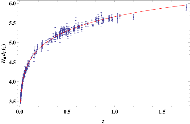
FIG. 3 is a representation of the observed luminosity distance for the 194 Sne Ia data and the corresponding model predicted theoretical value for . For evaluating theoretical we use CDM model parameters for and , i.e., we consider a small deviation of the CDM model, and, thus we get . We choose the interaction parameters, and throughout all estimations as per our assumption of very low interaction. From the figure it is clear that for these values of the parameter, our model gives a good fit to the data.
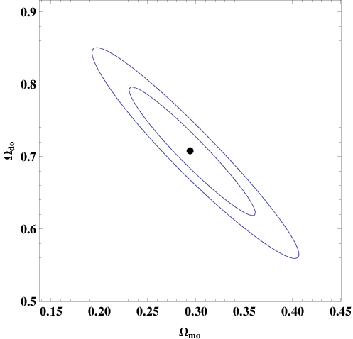
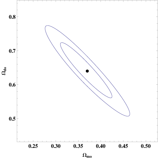
FIG. 4 shows the and contours in plane, and plane respectively. In all these results we have found that the best fit values of the free parameters and are consistent with the data. Thus, from the observational constraints we can conclude that the long term expansion history of the universe is overall in harmony with the existing models like CDM.

III.2 Observational constraints for variable
For variable restricted by Eq. (37), we have
| (59) |
where and can be found in (44) and (45) respectively. In this case also, the parameters and are nothing but the density parameters for the hypothetical non-interacting two fluids with values similar to and respectively. The new parameter (any real number) arises due to the choice of that makes it variable and as a result we can realize the different cosmic stages with the restrictions on the model parameters shown in Table I. FIG. 5 shows the and contours in plane for three different values of .
IV Cosmography of interacting dark energy
The idea of cosmography in cosmology was motivated after the introduction of the statefinder parameters by Sahni et al. [45]. The interesting fact behind the statefinder parameters are that, they are dimensionless geometrical, and model independent in nature. As a result, they were widely used to filter the observationally sound dark energy models among the various theoretical DE models in the literature. The statefinder parameters are defined as
| (60) |
Subsequently, this geometric investigation was extended by considering the Taylor series expansion of the scale factor about the present time in the following manner:


| (61) |
where we have some model independent and dimensionless parameters known as the cosmographic parameters [46, 47] defined in the following way:
| (62) |
The suffix ‘’ stands for the value of the corresponding variable at the present epoch (). The cosmographic parameters (from now we shall call these CP) are individually named as jerk () (this ‘’ is same as ‘’ defined by Sahni et al. [45]), snap () (this ‘’ is different from one defined by Sahni et al. [45]), lerk, and parameter [46, 47]. Further, the above CP can be expressed in terms of the deceleration parameter (), and, its higher derivatives:
| (63) | |||||
| (64) | |||||
| (65) | |||||
| (66) |
Thus, the evolution of the CP can be traced out only if and its higher derivatives are differentiable throughout the entire cosmic history. In FIGs. 6 and 7, we have shown the variations of the CP with the evolution of universe for constant and variable equation of state parameters respectively. From the figures, one can notice that during the entire evolution of the universe, the nature of and are almost same in sign, similar behavior is found for the parameters and .


V Summary of the work
The present work proposes a theoretical model of dark energy to match with recent observational evidences. Here, the dark energy is chosen in the form of perfect fluid with barotropic equation of state, and, it interacts non-gravitationally with dark matter chosen as dust. Analytic solutions are obtained both for constant and variable equation of state for DE with phenomenological choice for the interaction term. The asymptotic behavior of the relevant physical parameters are discussed and their variations have been shown graphically. These theoretical models are then compared with 194 available Supernovae data by Tonry et al. [33] and Barris et al. [34]. Using test for goodness of fit, the best fit values for the parameters are estimated, and, they are well accord with observed 1 (or, 2) level. For variable , the effect of DE is negligible at early universe, and, it starts dominating in recent past. Also, the estimated value of nicely matches with the very recently released Planck data set [42]. Therefore, this particular interacting DE model can be considered as an alternative for CDM model. Finally, the variation of the cosmographic parameters are presented graphically for both the theoretical models for different choices of the parameters involved. Finally, as the present model includes only CDM and DE as the two main ingredients, one can include the baryonic matter and radiation to the picture [48] in future such that the era of the creation of baryonic matter and radiation is built into the model.
VI Acknowledgments
SP acknowledges CSIR, Govt of India for financial support through SRF scheme (File No. 09/096 (0749)/2012- EMR-I). SB acknowledges UGC’s Faculty Recharge Programme. SC thanks UGC-DRS programme at the Department of Mathematics, Jadvapur University. SP thanks R. Erdem for some critical comments on the manuscript. SP also thanks S. Das for useful discussions in understanding the numerical programs. Finally, the authors are thankful to the referee whose critical comments helped us to improve the manuscript considerably.
References
- [1] A. G. Riess et al., “Observational evidence from supernovae for an accelerating universe and a cosmological constant”, Astron. J., 116, 1009 (1998) (arXiv: astro-ph/9805201).
- [2] S. Perlmutter et al., “Measurements of Omega and Lambda from 42 high redshift supernovae”, Astrophys. J., 517, 565 (1999) (arXiv: astro-ph/9812133).
- [3] D. N. Spergel et al., “First year Wilkinson Microwave Anisotropy Probe (WMAP) observations: Determination of cosmological parameters”, Astrophys. J. Suppl. 148, 175 (2003) (arXiv: astro-ph/0302209).
- [4] M. Tegmark et al., “Cosmological parameters from SDSS and WMAP”, Phys. Rev. D 69, 103501 (2004) (arXiv: astro-ph/0310723).
- [5] D. J. Eisenstein et al., “Detection of the baryon acoustic peak in the large-scale correlation function of SDSS luminous red galaxies”, Astrophys. J. 633, 560 (2005) (arXiv: astro-ph/0501171).
- [6] B. Jain and A. Taylor, “Cross-correlation tomography: measuring dark energy evolution with weak lensing”, Phys. Rev. Lett. 91, 141302 (2003) (arXiv: astro-ph/0306046).
- [7] S. Weinberg, “The Cosmological constant problem”, Rev. Mod. Phys. 61, 1 (1989).
- [8] S.M. Carroll, “The Cosmological Constant”, Living Rev. Relativ. 4, 1 (2001) (arXiv: astro-ph/0004075).
- [9] E. J. Copeland, M. Sami, and S. Tsujikawa, “Dynamics of dark energy”, Int. J. Mod. Phys. D 15, 1753 (2006) (arXiv: hep-th/0603057).
- [10] R. R. Caldwell, R. Dave, and P. J. Steinhardt, “Cosmological imprint of an energy component with general equation of state”, Phys. Rev. Lett. 80, 1582 (1998) (arXiv: astro-ph/9708069).
- [11] C. Armendariz-Picon, V. Mukhanov, and P. J. Steinhardt, “Essentials of k essence”, Phys. Rev. D 63, 103510 (2001) (arXiv: astro-ph/0006373).
- [12] T. Padmanabhan, “Accelerated expansion of the universe driven by tachyonic matter”, Phys. Rev. D 66, 021301 (2002) (arXiv: hep-th/0204150); A. Sen, “Remarks on tachyon driven cosmology”, Phys. Scr. T 117, 70 (2005) (arXiv: hep-th/0312153).
- [13] R. R. Caldwell, “A phantom menace? Cosmological consequences of a dark energy component with super-negative equation of state”, Phys. Lett. B 545, 23 (2002) (arXiv: astro-ph/9908168); R. R. Caldwell, M. Kamionkowski, and N. N. Weinberg, “Phantom energy and cosmic doomsday”, Phys. Rev. Lett. 91, 071301 (2003) (arXiv: astro-ph/0302506); M. Sami and A. Toporensky, “Phantom field and the fate of universe”, Mod. Phys. Lett. A 19 (2004) 1509 (arXiv: gr-qc/0312009).
- [14] E. Elizalde, S. Nojiri, and S. D. Odintsov, “Late-time cosmology in a (phantom) scalar-tensor theory: Dark energy and the cosmic speed-up”, Phys. Rev. D 70, 043539 (2004) (arXiv: hep-th/0405034).
- [15] B. Feng, X. L. Wang, and X. M. Zhang, “Dark energy constraints from the cosmic age and supernova”, Phys. Lett. B 607, 35 (2005) (arXiv: astro-ph/0404224).
- [16] Y.-F. Cai, E. N. Saridakis, M. R. Setare, and J.-Q. Xia, “Quintom Cosmology: Theoretical implications and observations”, Phys. Rept. 493, 1 (2010) (arXiv: 0909.2776 [hep-th]).
- [17] A. Kamenshchik, U. Moschella, and V. Pasquier, “An Alternative to quintessence”, Phys. Lett. B 511, 265 (2001) (arXiv: gr-qc/0103004); M. C. Bento, O. Bertolami, and A. A. Sen, “Generalized Chaplygin gas, accelerated expansion and dark energy matter unification”, Phys. Rev. D 66, 043507 (2002) (arXiv: gr-qc/0202064).
- [18] A. G. Cohen, D. B. Kaplan, and A. E. Nelson, “Effective field theory, black holes, and the cosmological constant”, Phys. Rev. Lett. 82, 4971 (1999) (arXiv: hep-th/9803132).
- [19] M. Li, “A Model of Holographic Dark Energy”, Phys. Lett. B 603, 1 (2004) (arXiv: hep-th/0403127).
- [20] C. Wetterich, “The cosmon model for an asymptotically vanishing time-dependent cosmological constant”, Astron. Astrophys. 301, 321 (1995) (arXiv: hep-th/9408025).
- [21] L. Amendola, “Coupled quintessence”, Phys. Rev. D 62, 043511 (2000) (arXiv: astro-ph/9908023).
- [22] L. Amendola, “Perturbations in a coupled scalar field cosmology”, Mon. Not. R. Astron. Soc. 312, 521 (2000) (arXiv: astro-ph/9906073).
- [23] A. P. Billyard and A. A. Coley, “Interactions in scalar field cosmology”, Phys. Rev. D 61, 083503 (2000) (arXiv: astro-ph/9908224).
- [24] W. Zimdahl, D. Pavon, and L. P. Chimento, “Interacting quintessence”, Phys. Lett. B 521, 133 (2001) (arXiv: astro-ph/0105479).
- [25] R. Herrera, D. Pavon, and Winfried Zimdahl, “Exact solutions for the interacting tachyonic dark matter system”, Gen. Relt. Grav. 36, 2161 (2004) (arXiv: astro-ph/0404086).
- [26] L.Amendola and C. Quercellini, “Tracking and coupled dark energy as seen by WMAP”, Phys. Rev. D 68, 023514 (2003) (arXiv: astro-ph/0303228).
- [27] M.B. Hoffman, “Cosmological constraints on a dark matter–dark energy interaction” (arXiv: astro-ph/0307350).
- [28] L. P. Chimento, A. S. Jakubi, D. Pavon, and W.Zimdahl, Interacting quintessence solution to the coincidence problem, Phys. Rev. D 67, 083513 (2003) (arXiv: astro-ph/0303145).
- [29] L. Amendola, “Linear and non-linear perturbations in dark energy models”, Phys. Rev. D 69, 103524 (2004) (arXiv: astro-ph/0311175).
- [30] A. Paliathanasis, M. Tsamparlis, “Two scalar field cosmology: Conservation laws and exact solutions”, Phys. Rev. D 90, 043529 (2014) (arXiv:1408.1798[gr-qc]).
- [31] Y.-F. Cai, H. Li, Y.-S. Piao, and X. Zhang, “Cosmic Duality in Quintom Universe”, Phys. Lett. B 646 (2007) 141 (arXiv: gr-qc/0609039).
- [32] S. Pan and S. Chakraborty, “A cosmographic analysis of holographic dark energy models”, Int. J. Mod. Phys. D 23, 1450092 (2014) (arXiv: 1410.8281 [gr-qc]).
- [33] J. L. Tonry et al., “Cosmological Results from High- Supernovae”, Astrophys. J. 594, 1 (2003) (arXiv: astro-ph/0305008).
- [34] B. J. Barris et al., “23 High Redshift Supernovae from the IfA Deep Survey: Doubling the SN Sample at ”, Astrophys.J. 602, 571 (2004) (arXiv: astro-ph/0310843).
- [35] J.-H. He and B. Wang, “Effects of the interaction between dark energy and dark matter on cosmological parameters”, J. Cosmol. Astropart. Phys 06, 010 (2008) (arXiv: 0801.4233 [astro-ph]).
- [36] M. Quartin et al., “Dark Interactions and Cosmological Fine-Tuning”, J. Cosmol. Astropart. Phys 05 (2008) 007 (arXiv: 0802.0546 [astro-ph]); G. Caldera-Cabral, R. Maartens, and L. A. Urena-Lopez, “Dynamics of interacting dark energy”, Phys. Rev. D 79, 063518 (2009) (arXiv: 0812.1827 [gr-qc]); C. G. Boehmer, G. Caldera-Cabral, R. Lazkoz, and R. Maartens, “Dynamics of dark energy with a coupling to dark matter”, Phys. Rev. D 78, 023505 (2008) (arXiv: 0801.1565 [gr-qc]).
- [37] L.P. Chimento, “Linear and nonlinear interactions in the dark sector”, Phys. Rev. D 81, 043525 (2010) (arXiv: 0911.5687 [astro-ph.CO]); L.P. Chimento, “Exactly solved models of interacting dark matter and dark energy”, AIP. Conf. Proc. 1471, 30 (2012), (arXiv: 1204.5797 [gr-qc]).
- [38] E. Komatsu et al., (WMAP Collaboration), “Seven-Year Wilkinson Microwave Anisotropy Probe (WMAP) Observations: Cosmological Interpretation”, Astrophys. J. Suppl. 192, 18 (2011) (arXiv: 1001.4538 [astro-ph.CO]).
- [39] P.A.R. Ade et al., “Planck 2013 results. XVI. Cosmological parameters”, Astron. Astrophys. 571, A 16 (2014) (arXiv: 1303.5076 [astro-ph.CO]).
- [40] J. A. Espichán Carrillo, J. M. Silva, J. A. S. Lima, “On the Quintessence Scalar Field Potential”, (arXiv: 0806.3299[gr-qc]).
- [41] A. Paliathanasis, M. Tsamparlis, S. Basilakos, and J.D. Barrow, “Dynamical analysis in scalar field cosmology”, Phys. Rev. D 91, 123535 (2015) (arXiv: 1503.05750[gr-qc]).
- [42] P.A.R. Ade et al., “Planck 2015 results. XIII. Cosmological parameters”, (arXiv: 1502.01589 [astro-ph.Co]).
- [43] S. Pan and S. Chakraborty, “Will there be again a transition from acceleration to deceleration in course of the dark energy evolution of the universe?”, Eur. Phys. J. C 73, 2575 (2013) (arXiv: 1303.5602 [gr-qc]).
- [44] L. Perivolaropoulos and S. Nesseris, http://leandros.physics.uoi.gr/cosmofit.htm.
- [45] V. Sahni, T. D. Saini, A. A. Starobinsky, and U. Alam, “Statefinder – a new geometrical diagnostic of dark energy”, J. Expo. Theor. Phys. Lett. 77, 201 (2003) (arXiv: astro-ph/0201498).
- [46] M. Visser, “Jerk and the cosmological equation of state”, Class. Quant. Grav. 21, 2603 (2004) (arXiv: gr-qc/0309109).
- [47] M. Visser, “Cosmography: Cosmology without the Einstein equations”, Gen. Relativ. Gravit. 37, 1541 (2005) (arXiv: gr-qc/0411131).
- [48] R. Erdem, “Single scale factor for the universe from the creation of radiation and matter till the present”, Eur. Phys. J. C 74, 3066 (2014) (arXiv: 1407.7199 [gr-qc]).