Mode bifurcation in the Rayleigh-Taylor instability of binary condensates

For linear stability analysis of the interface modes due to a small perturbation, to identify the onset of RTI, we transform the Eq. (14) to elliptic cylindrical coordinates $\displaystyle(u,v)$. Here, the coordinate $\displaystyle v$ represent the asymptotic angle of confocal hyperbolic cylinders symmetrical about the x-axis. And, the $\displaystyle u$ coordinates are confocal elliptic cylinders centered on the origin[16]. The transformation is defined by the relations $\displaystyle x=a\cosh u\cos v$, and $\displaystyle y=a\sinh u\sin v$ and $\displaystyle a$ is the focal distance along $\displaystyle x$-axis. We take the coordinates on the $\displaystyle z=0$ plane as we consider the TBEC in 2D. The Eq. (14) then assumes the form

where $\displaystyle\phi$ is the solution of the form $\displaystyle\phi=U(u)\Theta(v)$. Substituting, $\displaystyle\phi$ back in Eq.(15) we get,

Using separation of variables, the equation is simplified to the Mathieu equations [17, 16]

where, $\displaystyle{\mathcal{A}}=A+a^{2}k^{2}/2$ and $\displaystyle q=a^{2}k^{2}/4$. Here $\displaystyle A$ is the separation constant and returning to the earlier definition of the trapping potential, the anisotropy parameter $\displaystyle\alpha=\beta/\gamma$. The interface is an ellipse with eccentricity $\displaystyle e=\sqrt{1-1/\alpha^{2}}$ and from the theory of conic sections $\displaystyle a=\beta e=\sqrt{\alpha}e$. Based on these definitions, the constants in the Eq. (17) and (18) are redefined as

The constants in this form are easier to connect with the parameters of trapping potentials. The Eqns.(17 and 18) then assumes the form

The interface of the TBEC, an ellipse, has fixed coordinate $\displaystyle u$ representing the elliptic cylinder. But the angle coordinate $\displaystyle v$ varies and lies in the domain $\displaystyle[0,2\pi)$. Thus $\displaystyle\Theta$, solutions of the second equation, represent the normal modes of the interface. For circular interface, $\displaystyle\alpha=1$ and $\displaystyle e=0$, only $\displaystyle 0<A$ is physically admissible and the solution of the equation is reduced to sinusoidal functions.

For TBEC in traps, the gradient of the trapping potential is like the gravitational force in the conventional fluid dynamics and the flows within TBEC is modelled as potential flows. Consider the interface of the TBEC, using the method of normal modes, any arbitrary disturbance on the interface may be resolved into independent modes of the form

Here, $\displaystyle\xi$ is the position of the interface relative to the equilibrium configuration, and $\displaystyle\phi_{i}^{{}^{\prime}}$ is the increments in the velocity potential of the $\displaystyle i$th species about the interfacial region caused due to disturbance in the system. $\displaystyle\hat{\xi}$ and $\displaystyle\hat{\phi_{i}}$ are the amplitude of the modes and $\displaystyle s$ is the temporal decay constant.

We know that for an incompressible fluid, the Laplacian of the velocity potential vanishes $\displaystyle\nabla^{2}\phi_{i}^{{}^{\prime}}=0$ and from the expression of the normal modes

Using separation of variables, Eq.(26) can be simplified to,

where, $\displaystyle C^{2}=-(1/\Theta)(\partial^{2}\Theta/\partial v^{2})$. The general solution of the above equation in the regions of the two species are

where, $\displaystyle A_{1}$, $\displaystyle B_{1}$, $\displaystyle A_{2}$, $\displaystyle B_{2}$ are arbitrary constants. Here, it is to be noted that the sign of the exponents in the two solutions are interchanged. This is to indicate that the relative distance from the interface, within the two species, are in opposite directions. We may recall that the instabilities occur only at the interface or close to it. At any point far removed from the interface the normal modes must decay to zero. Thus, normal modes are of the form $\displaystyle\hat{\phi_{1}}=A_{1}\exp(-Cu)$ and $\displaystyle\hat{\phi_{2}}=A_{2}\exp(Cu)$. The velocity potentials in Eq.(24) and Eq.(25) are then

The dynamical evolution of the interface is described through a combination of the continuity equation, Euler’s equation and Bernoulli’s theorem[18, 3]. For stability analysis of the interface, we linearize these equations and neglect quadratic terms in $\displaystyle\phi_{1}^{{}^{\prime}}$, $\displaystyle\phi_{2}^{{}^{\prime}}$ and $\displaystyle\xi$. After linearization, we get

where, $\displaystyle g$ is the gradient of the trapping potential $\displaystyle V(x,y)$. On the interface, using the solutions obtained earlier, from Eq. (32) one can show that

In a similar way, from Eq. (31), we obtain $\displaystyle A_{1}=-s\hat{\xi}/C$ and $\displaystyle A_{2}=s\hat{\xi}/C$. Using these values in the above equation

Simplifying this equation, one arrives at the definition of the temporal decay constant

The densities of the condensates $\displaystyle n_{1}$ and $\displaystyle n_{2}$ are at a point $\displaystyle(u,v)$ on the interface. We recollect that $\displaystyle n_{2}$ refer to the density of species at the center which is surrounded by the species with density $\displaystyle n_{1}$. The interface is stable when $\displaystyle s$ is imaginary ( $\displaystyle n_{1}<n_{2}$) and oscillates when perturbed. However, when $\displaystyle n_{1}>n_{2}$, the value of $\displaystyle s$ is real and any perturbation, however small, grows exponentially with time. This is the prerequisite for RTI in binary condensates. In this context, Atwood number $\displaystyle{\Gamma}$ is given by [19]

¿From Eq. (22)

the temporal decay constant is then

where for compact notation we have used the relation $\displaystyle q=k^{2}e^{2}\alpha/4$ given earlier. Thus Eq. 38 can be rewritten as

This shows that $\displaystyle s$ is a function of $\displaystyle v$, the angular coordinate.

The solutions of Eq. (22), the angular Mathieu equation, are the $\displaystyle{\rm ce}_{\nu}(v,q)$ and $\displaystyle{\rm se}_{\nu}(v,q)$ functions [20], cosine and sine elliptic functions, respectively. Here, $\displaystyle\nu$ is real number and denotes the order of the elliptic functions. The solutions, however, exist only for certain range of $\displaystyle a$ and $\displaystyle q$, and these are shown as shaded regions in Fig. 3. In the figure, the shaded region consists of lobes and each are bounded by elliptic function of integer orders $\displaystyle{\rm ce}_{n-1}(v,q)$ and $\displaystyle{\rm se}_{n}(v,q)$, where $\displaystyle n=1,2,3,\ldots$. For the present case, when RTI sets in, the mushroom shaped superfluid flows have four fold symmetry in the case of circular symmetry. So that the flow retains symmetry or shape invariance along perpendicular directions. The corresponding solution of Eq. (22) which satisfy this condition is then $\displaystyle{\rm ce}_{2}(v,q)$, and it has the properties $\displaystyle{\rm ce}_{2}(v,q)={\rm ce}_{2}(v+\pi,q)$ and $\displaystyle{\rm ce}_{2}(v,q)={\rm ce}_{2}(-v,q)$. The loci of the $\displaystyle a$-$\displaystyle q$ pairings which allow this solution is the labeled curve in Fig. 3.

One property of $\displaystyle{\rm ce}_{2}(v,q)$ is, the maximum at $\displaystyle v=0$ undergoes a smooth bifurcation at higher values of $\displaystyle q$. Coming to the description of the interface in the binary condensates, from Eq. (19), $\displaystyle q$ is a linear function of the anisotropy parameter $\displaystyle\alpha$. So, as we increase the anisotropy the mushroom shaped flows in RTI must undergo bifurcation. At some value of $\displaystyle\alpha$, instead of four there must be six mushroom shaped inward superfluid flow.

We consider a system of ⁸⁵Rb–⁸⁷Rb atoms in a symmetric 2-D harmonic trapping potential with ($\displaystyle\omega_{\perp},\omega_{z}$) = $\displaystyle 2\pi\times(8,90){\rm Hz}$. We choose initial state to be the ground state for which $\displaystyle a_{11}=460a_{\rm B}$, $\displaystyle a_{22}=99a_{\rm B}$, $\displaystyle a_{12}=a_{21}=214a_{\rm B}$, with $\displaystyle a_{\rm B}$ being the Bohr radius. The number of atoms are $\displaystyle N_{1}=5\times 10^{5}$ and $\displaystyle N_{2}=10^{6}$ [22]. In this configuration, component 1(outer), ⁸⁵Rb completely surrounds component 2(inner), ⁸⁷Rb. Fig. 1 shows phase separated profiles of the TBEC at $\displaystyle t=0$ in a perfectly symmetric pancake shaped trap i.e. $\displaystyle\alpha=1$.

Now, the $\displaystyle s$-wave scattering length $\displaystyle a_{11}$ of the outer species is decreased gradually over time, experimentally this is possible through the ⁸⁵Rb-⁸⁵Rb magnetic Feshbach resonance[23]. However, throughout the process, we maintain $\displaystyle({\mathcal{N}}_{12}>\sqrt{{\mathcal{N}}_{11}{\mathcal{N}}_{22}})$ so that the TBEC remains in the immiscible domain. A stage is reached when $\displaystyle a_{11}<a_{22}$, ⁸⁵Rb-⁸⁵Rb interaction weaker than the ⁸⁷Rb-⁸⁷Rb interaction. In this situation, the existing spatial structure of the system is energetically unfavourable and the outer species starts penetrating inside the inner species. Instabilities begin to occur at the interface of the two components and eventually grows into a four fold mushroom shape superfluid flow as shown in Fig. 4

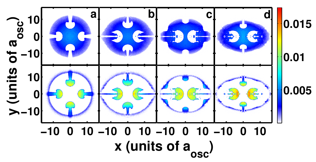
The dynamics and the formation of lobes also depends on the geometry of the interface. As the anisotropy of the trap $\displaystyle\alpha$ is increased keeping $\displaystyle\lambda$ and other remaining parameters fixed, the circular interface evolves into an elliptic interface. The penetration of the heavier fluid into the lighter fluid gets initiated along the $\displaystyle x$-axis, followed by the formation of lobes. This happens because, the interface is more curved along this direction with less confinement. Larger is the curvature, higher is the rate of inflow of the heavier fluid. Mass transport gradually occurs along $\displaystyle y$-direction, which is tightly confined. The interface here, is relatively flat and the lobes are formed at later stages of evolution. This is clearly evident from the superfluid flow pattern soon after the onset of RTI as shown in Fig. 5. In Fig. 5c-d, the lobes of $\displaystyle n_{2}$ along the $\displaystyle x$-axis are well developed and located deep within $\displaystyle n_{1}$. As $\displaystyle\alpha$ is increased further, the interface is deformed further. The lobe along the $\displaystyle y$-axis undergoes a bifurcation when the anisotropy is such that $\displaystyle\alpha=3$ and the density profile of the superfluid flow is shown in Fig. 6. Taking an average along the interface and close to the bulk of $\displaystyle n_{1}$, when the mode bifurcates the value of $\displaystyle\tilde{\mu}$ is 5.25. This can be related qualitatively to the analytic results, in which case $\displaystyle{\rm ce}_{2}(v,q)$ undergoes bifurcation at around $\displaystyle q\approx 3.7$. Thus our numerical results is in agreement with the inferences drawn from the analytic solutions of the interface modes.

For a more detailed understanding of the instability, we perform a Bogoliubov analysis for TBEC in a 2-D harmonic trap. Setting, $\displaystyle\Phi_{i}=\phi_{i}+\delta\phi_{i}$, we expand the set of coupled GP equations in Eq. 9 in $\displaystyle\delta\phi_{i}(x,y)$. Here, $\displaystyle\phi_{i}$’s fixes the condensate density through $\displaystyle n_{i}(x,y)=|\phi_{i}(x,y)|^{2}$ and $\displaystyle\delta\phi_{i}$’s are the deviations from the initial ground state, which includes the quasi-particle excitations. We consider excitation mode of the form

where, $\displaystyle\mu_{i}$ is the chemical potential, $\displaystyle\omega$ is the excitation frequency, and $\displaystyle u_{i}$ and $\displaystyle v_{i}$ are the Bogoliubov amplitudes. Using this ansatz, the Bogoliubov equations are

These equations are then numerically diagonalized to calculate the excitation spectrum. If the frequencies are real, the perturbations remain bounded and the system is dynamically stable. On the other hand, pure imaginary eigenfrequencies denote instability of the system. The eigenmode corresponding to this complex frequency grows exponentially and is a signature of dynamically unstable system [24].

As a case study, we choose $\displaystyle N_{2}/N_{1}=2$. For the isotropic case, $\displaystyle\alpha=1$, we expand the Bogoliubov amplitudes in harmonic oscillator basis wave function. When $\displaystyle\delta\phi_{i}$ is small, Re$\displaystyle(\omega)$ increases monotonically upto a critical point as the $\displaystyle a_{11}$ is decreased. When $\displaystyle a_{11}<a_{22}$ and RTI sets in, the low lying excitation modes $\displaystyle\omega$ starts becoming imaginary. The value of the Im$\displaystyle(\omega)$ increases monotonically as $\displaystyle a_{11}$ is decreased further and away from the critical point. These imaginary modes are signatures of instability in the dynamics of the binary condensates.

Numerical studies that have been carried out so far are at zero temperature and without any imperfections, hence quite ideal. But in experiments, conditions are far from ideal. Fluctuations play a major role, and if large, may destroy the observed signatures predicted from the numerical simulations. One immediate remedy is to include fluctuation to our calculations. We introduce white noise during the real time evolution of TBEC. The white noise is at the level of $\displaystyle 0.01\%$. Even after introducing noise, we still observe signatures of RTI as a result of changing $\displaystyle a_{11}$. The thermodynamical quantities such as energy, chemical potential may vary quantitatively, but, there is no qualitative difference in the shape of the interface after RTI is initiated. Bifurcation of normal modes on the interface are still observed at the predicted values of the anisotropy of the trap.