The space of measured foliations of the hexagon

We consider foliations on the hexagon, with isolated singularities with $3$ separatrices and such that no leaf is homotopic to a point. There may be zero or one singularity in the hexagon (see Figure 1). In particular, the five configurations in Figure 2 are excluded.

We consider a hexagon $H$ whose sides are denoted in cyclic order by $a,C,b,A,c,B$ ($a$ opposite to $A$, etc.)

An arc in the hexagon $H$ is the homeomorphic image of a closed interval, whose interior is in the interior of $H$ and whose endpoints are on $\partial H$.

An arc triple is a triple of disjoint arcs each joining two non-adjacent boundary edges of the hexagon. Up to homotopy, there are 14 arc triples in the hexagon, and some of them are represented in Figure 3. The names of the other arcs are obtained similarly. In Figure 3, the arc $\beta$ joins $b$ to $B$. The notation for the other arcs is analogous, with a cyclic change in names. That is, the arc $\alpha$ joins $a$ to $A$, and the arc $\gamma$ joins $c$ to $C$.

Such a foliation $F$ is equipped with an invariant transverse measure, in the sense of [2]. The geometric intersection number, $i(F,\partial)$ of $F$ with an arc $\partial$ in the hexagon is the infimum of the transverse measure with $F$ of an arc homotopic to $\partial$.

We denote by $\mathcal{MF}$ the space of measured foliations of the hexagon up to homotopy. We equip $\mathcal{MF}$ with the quotient topology induced by the geometric convergence of representatives together with convergence of transverse measures on arcs. We denote by $\mathcal{PMF}$ the quotient space of $\mathcal{MF}$ by the natural action of the positive reals $\mathbb{R}_{+}$.

A measured foliation (or its equivalence class in $\mathcal{MF}$) is said to be in good position with respect to an arc triple $\{\partial_{1},\partial_{2},\partial_{3}\}$ if

1. (1)

   $\displaystyle\sum_{j=1}^{3}i(F,\partial_{j})>0$ ;

2. (2)

   $F$ has no leaf parallel to one of the three arcs in the triple $\{\partial_{1},\partial_{2},\partial_{3}\}$.

The first condition is equivalent to the fact that at least one of the arcs $\partial_{1},\partial_{2},\partial_{3}$ has positive $F-$measure.

An example is given in Figure 4.

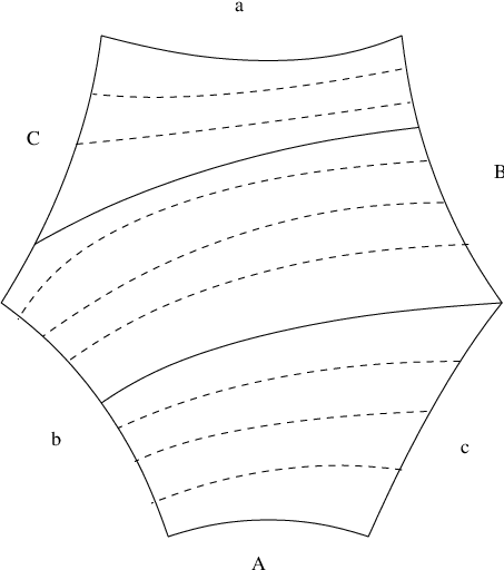
The behavior of measured foliations in good position with respect to an arc triple $\{\partial_{1},\partial_{2},\partial_{3}\}$ is conveniently described by the projective space of transverse measures, see Figure 5.

In what follows, we shall often draw partial foliations, that is, foliations whose support is a subsurface of the hexagon; it will be clear from the picture how one has to collapse the non-foliated regions in order to obtain a measured foliation which is well-defined up to equivalence.

We shall denote by $\mathcal{MF}_{\partial}$ and $\mathcal{PMF}_{\partial}$ the subspaces of $\mathcal{MF}$ and $\mathcal{PMF}$ respectively of equivalence classes of measured foliations that are in good position with respect to an arc triple $\partial$.

We have $\mathcal{MF}=\mathcal{MF}_{\{a,b,c\}}\cup\mathcal{MF}_{\{A,B,C\}}\cup\mathcal{MF}_{\{a,\beta,c\}}\cup\mathcal{MF}_{\{a,b,\gamma\}}\cup\ldots$

We shall gather the subsets $\mathcal{PMF}_{\partial}$ associated to the 14 possible arc triples in the following three categories:

The subsets $\mathcal{PMF}_{\partial}$ are local charts for $\mathcal{PMF}$ forming an atlas for this space. We shall show that the coordinate changes between local charts are piecewise-linear. This will show that $\mathcal{PMF}$ is a piecewise-linear manifold. We shall see that this manifold is homeomorphic to the 2-sphere.

In Figure 9, we have represented the coordinate changes. The maps $\phi_{i}$ are the coordinate change maps between the charts. In this figure, the charts are represented in the projective space, but they have to be thought of as being in $\mathcal{MF}$. The charts are triangular, and there are two sorts of coordinate changes:

1. (1)

   The intersection of the two charts (the domain and range of the map $\phi_{i}$) has nonempty interior. In this case the intersection is left blank in the figure.

2. (2)

   The intersection of the two charts has empty interior. In this case, the intersection is along the boundary, and in the figure this intersection is represented in thicker lines.

From the following formulae for the coordinate changes we can see that they are piecewise-linear. There are five cases, corresponding to the cases drawn in Figure 9. Let us consider as an example the case of $\phi_{2}$: this is the coordinate change map which maps the non-hachured part of the triangle $(a,b,c)$ on the left to the non-hachured part of the triangle $(\alpha,b,c)$ on the right. These two pieces coincide as subsets of $\mathcal{MF}$ since they contain the same foliations. The non-hachured part of the triangle $(a,b,c)$ is subdivised into three triangular subparts (numbered 1, 2, 3). The map $\phi_{2}$ is linear on each of these subparts in the parameters $a,b,c$ (see the corresponding formulae, in which $(\alpha,b,c)$ stand for the parameters in the image triangle). The map $\phi_{2}$ is therefore piecewise-linear on the non-hachured part of the triangle $(a,b,c)$ on the left. The same holds for the other triangles.

1. (1)

   Formula for $\phi_{1}$: If $b\geq c$, then $\begin{cases}\alpha=b\\ B=b-c\\ C=0\end{cases}$ and if $b\leq c$, then $\begin{cases}\alpha=c\\ B=0\\ C=c-b\end{cases}$

2. (2)

   Formula for $\phi_{2}$: If $(a,b,c)$ is in the region labelled 1, then $\begin{cases}\alpha=\frac{1}{2}(b+c-a)\\ b=b\\ c=c\end{cases}$

   and if $(a,b,c)$ is in the region labelled 2, then $\begin{cases}\alpha=b-a\\ b=b\\ c=c\end{cases}$

   and if $(a,b,c)$ is in the region labelled 3, then $\begin{cases}\alpha=c-a\\ b=b\\ c=c\end{cases}$

3. (3)

   Formula for $\phi_{3}$: If $a\geq b+c$ , then $\begin{cases}\beta=a-b\\ a=a\\ A=a-b-c\end{cases}$ ($a>\beta>A$).

4. (4)

   Formula for $\phi_{4}$: If $\alpha>c$ , then $\begin{cases}\alpha=\alpha\\ b=b\\ B=\alpha-c\end{cases}$

5. (5)

   Formula for $\phi_{5}$: If $C>B$ and $A=0$, then $\begin{cases}\alpha=C\\ b=0\\ c=C-B\end{cases}$ ;

   if $C<B$ and $A=0$, then $\begin{cases}\alpha=B\\ b=B-C\\ c=0\end{cases}$

Figure 10 represents the space $\mathcal{PMF}$, which is homeomorphic to a sphere, represented in the plane with a point at infinity. The small star $ABC$ is the chart $\mathcal{PMF}_{\{a,b,c\}}$, and the exterior of the big star $IAKCJB$ is the chart $\mathcal{PMF}_{\{A,B,C\}}$. Its centre is at infinity.

The other charts are polygons whose edges are contained in the graph that is drawn.

Using this and the fact that $\mathcal{PMF}_{\{a,b,c\}}\cap\mathcal{PMF}_{\{A,B,C\}}$ is constituted of the three vertices of each triangle, Figure 10 shows that $\mathcal{PMF}$ is a sphere equipped with a natural piecewise-linear structure. In fact, more than that, it is equipped with a natural triangulation. In Figure 10, the centre of the triangle $\mathcal{PMF}_{\{A,B,C\}}$ is at infinity and the centre of the triangle $\mathcal{PMF}_{\{a,b,c\}}$ is at 0.

We denote by $\mathcal{T}$ the Teichmüller space of the right hexagon. As we shall presently prove, a point in $\mathcal{T}$ is determined by the three lengths of any fixed arc triple, for instance $\{a,b,c\}$.

Let $\partial=\{\partial_{1},\partial_{2},\partial_{3}\}$ be a fixed arc triple of the right hexagon. Let

be the length functional associated to $\partial$.

For a coming proof, we recall right here the following well-known trigonometric formulae, [1] p. 85 and 86. (We use the notation of Figure 12).

Let us collect some asymptotic behaviors of the lengths of the sides of a right hexagon.

We shall say that a sequence $(x_{n})$ in $\mathcal{T}$ tends to infinity if there exists an arc $\partial_{j}$ of an arc triple $\partial$ such that $|\log l_{x_{n}}(\partial_{j})|\to\infty$ as $n\to\infty$.

The space $\mathcal{MF}$ is embedded in $\mathbb{R}^{6}_{\geq 0}$ using the intersection functional:

The space $\mathcal{T}$ is embedded in $\mathbb{R}^{6}_{>0}$ using the length functional:

The images $l_{*}(\mathcal{T})$ and $i_{*}(\mathcal{MF})$ are disjoint since for all $F\in\mathcal{MF}$ there is at least one component of $i_{*}(F)$ in $\mathbb{R}^{6}_{\geq 0}$ which is zero.

We denote by $\pi$ the projection map : $\mathbb{R}^{6}\setminus\{0\}\to{\rm P}\mathbb{R}^{6}.$ Let

By what precedes, $\pi\circ l_{*}(\mathcal{T})$ can be identified with Teichmüller space $\mathcal{T}$ itself while $\pi\circ i_{*}(\mathcal{MF})$ can be naturally identified with $\mathcal{PMF}$.

Let $\epsilon>0$ and let $\partial=\{\partial_{1},\partial_{2},\partial_{3}\}$ be an arc triple. Set

This subset is open in $\mathcal{T}$.

Let $\partial=\{\partial_{1},\partial_{2},\partial_{3}\}$ be an arc triple and let $\epsilon$ be a positive number. We consider the map

defined by foliating the right hexagon by leaves equidistant to certain arcs that do not belong to the arc triple $\partial$ in such a way that the transverse measure of each arc $\partial_{i}$ ($i=1,2,3$) coincides with its length, that is, $l_{h}(\partial_{i})=i(q_{\partial}^{\epsilon}(h),\partial_{i})>\epsilon$ for $i=1,2,3$. The injectivity of $q_{\partial}$ follows easily from Proposition 3.1.

We denote by $\stackrel{{\scriptstyle\circ}}{{\mathcal{PMF}_{\partial}}}$ the interior of $\mathcal{PMF}_{\partial}$. We describe local charts for $\overline{\mathcal{T}}$ around each point of $\stackrel{{\scriptstyle\circ}}{{\mathcal{PMF}_{\partial}}}$, and we show that this space is a manifold with boundary.

Consider the map

defined by

(Here, as elsewhere, we write $\partial_{1}$ instead of $l_{x}(\partial_{1})$, etc.) This maps defines, as the following propositions indicates, local coordinates for $\overline{\mathcal{T}}$ (see Figure 13).

Since $\mathcal{T}=\cup_{\partial}\mathcal{T}_{\partial}^{\epsilon}$ for some $\epsilon>0$, we have shown that $\overline{\mathcal{T}}$ is a manifold with boundary, bounded by $\mathcal{PMF}$.

We know that $\mathcal{PMF}$ is homeomorphic to a sphere. The interior of a collar neighborhood of $\mathcal{PMF}$ is a sphere embedded in the interior of $\mathcal{T}$, which is homeomorphic to a ball. From Schönflies’ theorem, this sphere bounds a ball. Thus, $\overline{\mathcal{T}}$ is homeomorphic to a three-dimensional closed ball. Let us summarize this in the following

We close this section by giving in Figure 14 a few examples of sequences of right hexagons converging towards the boundary, together with their limit points.

References

- [1] W. Fenchel, Elementary geometry in hyperbolic space, de Gruyter studies in Mathematics, 11, Walter de Gruyter & Co., 1989.
- [2] A. Fathi, F. Laudenbach and V. Poénaru, Travaux de Thurston sur les surfaces, Astérisque 66–67 (1979).
- [3] A. Papadopoulos and G. Théret, Some Lipschitz maps between hyperbolic surfaces with applications to Teichmüller theory, Geometriae Dedicata, online version: 31 January 2012, pp. 1-21
- [4] A. Papadopoulos, L. Liu, W. Su and G. Théret, Length spectra and the Teichmüller metric for surfaces with boundary, Monatshefte für Mathematik , 2010, vol. 161, no. 3, pp. 295–311
- [5] W. P. Thurston, Three-Dimensional Geometry and Topology, Volume 1, Princeton University Press, Princeton, New Jersey, 1997.