Compute-and-Forward Strategies for Cooperative Distributed Antenna SystemsThanks: This research was supported in part by the KCC (Korea Communications Commission), Korea, under the R&D program supervised by the KCA (Korea Communications Agency) (KCA-2011-11921-04001).

A cloud base station is a Distributed Antenna System (DAS) formed by a number of simple antenna terminals (ATs) [1], spatially distributed over a certain area, and connected to a central processor (CP) via wired backhaul [2, 3, 4]. Cloud base station architectures differ by the type of processing made at the ATs and at the CP, and by the type of wired backhaul. At one extreme of this range of possibilities, the ATs perform just analog filtering and (possibly) frequency conversion, the wired link are analog (e.g., radio over fiber [5]), and the CP performs demodulation to baseband, A/D and D/A conversion, joint decoding (uplink) and joint pre-coding (downlink). At the other extreme we have “small cell” architectures where the ATs perform encoding/decoding, the wired links send data packets, and the CP performs high-level functions, such as scheduling, link-layer error control, and macro-diversity packet selection.

In this paper we focus on an intermediate DAS architecture where the ATs perform partial decoding (uplink) or precoding (downlink) and the backhaul is formed by digital links of fixed rate $R_{0}$. In this case, the DAS uplink is an instance of a multi-source single destination layered relay network where the first layer is formed by the user terminals (UTs), the second layer is formed by the ATs and the third layer contains just the CP (see Fig. 1). The corresponding DAS downlink is an instance of a broadcast layered relay network with independent messages.

In our model, analog forwarding from ATs to CP (uplink) or from CP to ATs (downlink) is not possible. Hence, some form of quantization and forwarding is needed. A general approach to the uplink is based on the Quantize reMap and Forward (QMF) paradigm of [6] (extended in [7] where it is referred to as Noisy Network Coding). In this case, the ATs perform vector quantization of their received signal at some rate $R^{\prime}\geq R_{0}$. They map the blocks of $nR^{\prime}$ quantization bits into binary words of length $nR_{0}$ by using some randomized hashing function (notice that this corresponds to binning if $R^{\prime}>R_{0}$), and let the CP perform joint decoding of all UTs’ messages based on the observation of all the (hashed) quantization bits.¹¹ 1 The information-theoretic vector quantization of [6], [7] can be replaced by scalar quantization with a fixed-gap performance degradation [8]. It is known [6] that QMF achieves a rate region within a bounded gap from the cut-set outer bound [9], where the bound depends only on the network size and on $R_{0}$, but it is independent of the channel coefficients and of the operating SNR. For the broadcast-relay downlink, a general coding strategy has been proposed in [10] based on a combination of Marton coding for the general broadcast channel [11] and a coding scheme for deterministic linear relay networks, “lifted” to the Gaussian case. Specializing the above general coding schemes to the the DAS considered here, for the uplink we obtain the scheme based on quantization, binning and joint decoding of [12], and for the downlink we obtain the Compressed Dirty-Paper Coding (CDPC) scheme of [13]. From an implementation viewpoint, both QMF and CDPC are not practical, the former requiring vector quantization at the ATs and joint decoding of all UT messages based on the hashed quantization bits at the CP, and the latter requiring Dirty-Paper Coding (notoriously difficult to implement in practice) and vector quantization at the CP.

A lower complexity alternative strategy for general relay networks was proposed in [14] and goes under the name of Compute and Forward (CoF). CoF makes use of lattice codes, such that each relay can reliably decode a linear combination with integer coefficient of the interfering codewords. Thank to the fact that lattices are modules over the ring of integers, this linear combination translates directly into a linear combination of the information messages defined over a suitable finite field. CoF can be immediately used for the DAS uplink. The performance of CoF was examined in [15] for the DAS uplink in the case of the overly simplistic Wyner model [16]. It was shown that CoF yields competitive performance with respect to QMF for practically realistic values of SNR.

This paper contributes to the subject in the following ways: 1) for the DAS uplink , we consider the CoF approach and examine the corresponding system optimization at finite SNR for a general channel model including fading and shadowing (i.e., beyond the nice and regular structure of the Wyner model); 2) For the downlink, we propose a novel precoding scheme nicknamed Reverse Compute and Forward (RCoF); 3) For both uplink and downlink, we present low-complexity versions of CoF and RCoF based on standard scalar quantization at the receivers. These schemes are motivated by the observation that the main bottleneck of a digital receiver is the Analog to Digital Conversion (ADC), which is costly, power-hungry, and does not scale with Moore’s law. Rather the number of bit per second produced by an ADC is roughly a constant that depends on the power consumption [17, 18]. Therefore, it makes sense to consider the ADC as part of the channel. The proposed schemes, nicknamed Quantized CoF (QCoF) and Quantized RCoF (RQCoF), lead to discrete-input discrete-output symmetric memoryless channel models naturally matched to standard single-user linear coding. In fact, QCoF and RQCoF can be easily implemented using $q$-ary Low-Density Parity-Check (LDPC) codes [19, 20, 21] with $q=p^{2}$ and $p$ prime, yielding essentially linear complexity in the code block length and polynomial complexity in the system size (minimum between number of ATs and UTs).

The two major impairments that deteriorate the performance of DAS with CoF/RCoF are the non-integer penalty (i.e., the residual self-interference due to the fact that the channel coefficients take on non-integer values in practice) and the rank-deficiency of the resulting system matrix over the $q$-ary finite field. In fact, the wireless channel is characterized by fading and shadowing. Hence, the channel matrix from ATs to UTs does not have any particularly nice structure, in contrast to the Wyner model case, where the channel matrix is tri-diagonal [15]. Thus, in a realistic setting, the system matrix resulting from CoF/RCoF may be rank deficient. This is especially relevant when the size $q$ of the finite field is small (e.g., it is constrained by the resolution of the A/D and D/A conversion). The proposed system optimization counters the above two problems by considering power allocation, network decomposition and antenna selection at the receivers (ATs selection in the uplink and UTs selection in the downlink). We show that in most practical cases the AT and UT selection problems can be optimally solved by a simple greedy algorithm. Numerical results show that, in realistic networks with fading and shadowing, the proposed optimization algorithms are very effective and essentially eliminate the problem of system matrix rank deficiency, even for small field size $q$.

A final novel contribution of this paper consists of the Integer-Forcing Beamforming (IFB) downlink scheme, targeted to the case where $R_{0}$ is large, and therefore the DAS downlink reduces to the well-known vector Gaussian broadcast channel. In this case, a common and well-known low-complexity alternative to the capacity-achieving Gaussian DPC scheme consists of Zero-Forcing Beamforming (ZFB), which achieves the same optimal multiplexing gain, at the cost of some performance loss at finite SNR. IFB can be regarded both as a generalization of ZFB and as the dual of Integer-Forcing Receiver (IFR), proposed in [22] for the uplink multiuser MIMO case. We demonstrate that IFB can achieve rates close to the information-theoretic optimal Gaussian DPC, and can significantly outperform conventional ZFB. This gain can be explained by the fact that IFB is able to reduce the power penalty of ZFB, due to non-unitary beamforming.

The paper is organized as follows. In Section II we define the uplink and downlink DAS system model, summarize some definitions on lattices and lattice coding, and review CoF. In Section III we consider the application of CoF to the DAS uplink and introduce the (novel) concept of network decomposition to improve the CoF sum rate. Section IV considers the DAS downlink and presents the RCoF scheme. In Section V we introduce the low-complexity “quantized” versions of CoF and RCoF. Section VI focuses on the symmetric Wyner model and presents a simple power allocation strategy to alleviate the impact of non-integer penalty. In the case of a realistic DAS channel model including fading, shadowing and pathloss, a low-complexity greedy algorithm for ATs selection (uplink) and UTs selection (downlink) is presented in Section VII. Finally, Section VIII considers the case of large backhaul rate and presents the IFB scheme. Some concluding remarks are provided in Section IX.

In this section we provide some basic definitions and results that will be extensively used in the sequel.

In this section we apply CoF to the DAS uplink and further improve its sum rate by introducing the idea of network decomposition. The scheme is illustrated in Fig. 2, where CoF is used at each AT receiver. For simplicity of exposition, we restrict to consider the same number $K=L$ of UTs and ATs. The notation, however, applies also to the case of $K<L$ addressed in Section VII, when considering AT selection. The UTs make use of the same lattice code ${\cal L}$ of rate $R$, and produce their channel input $\underline{{\bf x}}_{k}$, $k=1,\ldots,K$, according to (4). Each AT $\ell$ decodes the codeword linear combination $\underline{{\bf v}}_{\ell}=\left[\sum_{k=1}^{K}a_{\ell,k}\underline{{\bf t}}_{k}\right]\mod\Lambda$, for a target integer vector ${\bf a}_{\ell}=(a_{\ell,1},\ldots,a_{\ell,K})^{\sf T}\in\mbox{\bb Z}^{K}[j]$ determined according to Algorithm 1, independently of the other ATs. If $R\leq R({\bf h}_{\ell},{\bf a}_{\ell},{\sf SNR})$, where the latter denotes the computation rate of the G-MAC formed by the UTs and the $\ell$-th AT, taking on the form given in (8), the decoding error probability at AT $\ell$ can be made as small as desired. Letting $\underline{{\bf u}}_{\ell}=f^{-1}(\underline{{\bf v}}_{\ell})$ denote the information message corresponding to the target decoded codeword $\underline{{\bf v}}_{\ell}$, the code linearity over $\mbox{\bb F}_{p^{2}}$ and the $\mbox{\bb Z}[j]$-module structure of $\Lambda_{1}$ yield

where $q_{\ell,k}=g^{-1}([a_{\ell,k}]\mod p\mbox{\bb Z}[j])$. After decoding, each AT $\ell$ forwards the corresponding information message $\hat{\underline{{\bf u}}}_{\ell}$ to the CP via wired links of fixed $R_{0}$. This can be done if $R\leq R_{0}$. The CP collects all the messages $\hat{\underline{{\bf u}}}_{\ell}$ for $\ell=1,\ldots,L$ and forms the system of linear equations over $\mbox{\bb F}_{p^{2}}$

where we define ${\bf A}=[{\bf a}_{1},\ldots,{\bf a}_{L}]^{\sf T}$ and the system matrix ${\bf Q}=[{\bf q}_{1},\ldots,{\bf q}_{L}]^{{\sf T}}=g^{-1}\left([{\bf A}]\mod p\mbox{\bb Z}[j]\right)$. Provided that ${\bf Q}$ has rank $K$ over $\mbox{\bb F}_{p^{2}}$, the CP obtains the decoded messages $\{\hat{\underline{{\bf w}}}_{k}\}$ by Gaussian elimination. Assuming this full-rank condition and $R<R({\bf h}_{\ell},{\bf a}_{\ell},{\sf SNR})$ for all $\ell=1,\ldots,L$, the error probability $\mbox{\bb P}(\hat{\underline{{\bf w}}}_{k}\neq\underline{{\bf w}}_{k}\;\;\mbox{for some}\;k)$ can be made arbitrarily small for sufficiently large $n$. The resulting achievable rate per user is given by [15]:

The sum rate of CoF-based DAS can be improved by network decomposition with respect to the system matrix ${\bf Q}$. Although the elements of ${\bf H}$ are non-zero, the corresponding ${\bf Q}$ may include zeros, since some elements of the vectors ${\bf a}_{\ell}$ may be zero modulo $p\mbox{\bb Z}[j]$. Because of the presence of zero elements, the system matrix ${\bf Q}$ may be put in block diagonal form by column and row permutations. If the permuted system matrix has $S$ diagonal blocks, the corresponding network graph decomposes into $S$ independent subnetworks and CoF can be applied separately to each subnetwork such that taking the minimum of the computation rates over the subnetworks is not needed. Hence, the sum rate is given by the sum (over the subnetworks) of the sum rates of each network component. In turns, the common UT rate of each indecomposable subnetwork takes on the form (12). For given ${\bf Q}$, the disjoint subnetwork components can be found efficiently using depth-first or breadth-first search [28]. This also essentially reduces the computation complexity of Gaussian elimination, which is performed independently for each subnetwork. We assume that, up to a suitable permutation of rows and columns, ${\bf Q}$ can be put in block diagonal form with diagonal blocks ${\bf Q}({\cal A}_{s},{\cal U}_{s})$ for $s=1,\ldots,S$, where we use the following notation: for a matrix ${\bf Q}$ with rows index set $[1:L]$ and column index set $[1:K]$, ${\bf Q}({\cal A},{\cal U})$ denotes the submatrix obtained by selecting the rows in ${\cal A}\subseteq[1:L]$ and the columns in ${\cal U}\subseteq[1:K]$. The following results are immediate:

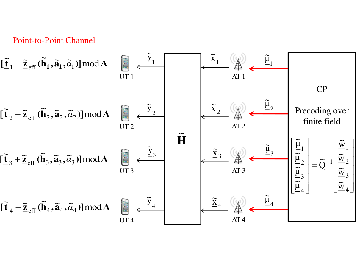
In this section we propose a novel downlink precoding scheme nicknamed “Reverse” CoF (RCoF). Again, we restrict to the case $K=L$ although the notation applies to the case of $K>L$, treated in Section VII. In a DAS downlink, the role of the ATs and UTs can be reversed with respect to the uplink. Each UT can reliably decode an integer linear combination of the lattice codewords sent by the ATs. However, the UTs cannot share the decoded codewords as in the uplink, since they have no backhaul links. Instead, the “interference” in the finite-field domain can be totally eliminated by zero-forcing precoding (over the finite field) at the CP. RCoF has a distinctive advantage with respect to its CoF counterpart viewed before: since each UT sees only its own lattice codeword plus the effective noise, each message is rate-constrained by the computation rate of its own intended receiver, and not by the minimum of all computation rates across all receivers, as in the uplink case. In order to achieve different coding rates while preserving the lattice $\mbox{\bb Z}[j]$-module structure, we use a family of nested lattices $\Lambda\subseteq\Lambda_{L}\subseteq\cdots\subseteq\Lambda_{1}$, obtained by a nested construction A as described in [14, Sect. IV.A]. In particular, we let $\Lambda_{\ell}=p^{-1}g({\cal C}_{\ell}){\bf T}+\Lambda$ with $\Lambda=\mbox{\bb Z}^{n}[j]{\bf T}$ and with ${\cal C}_{\ell}$ denoting the linear code over $\mbox{\bb F}_{p^{2}}$ generated by the first $r_{\ell}$ rows of a common generator matrix ${\bf G}$, with $r_{L}\leq r_{L-1}\leq\cdots\leq r_{1}$. The corresponding nested lattice codes are given by ${\cal L}_{\ell}=\Lambda_{\ell}\cap{\cal V}_{\Lambda}$, and have rate $R_{\ell}=\frac{2r_{\ell}}{n}\log p$. We let $\tilde{{\bf A}}=[\tilde{{\bf a}}_{1},\ldots,\tilde{{\bf a}}_{K}]^{{\sf T}}$, where $\tilde{{\bf a}}_{k}\in\mbox{\bb Z}^{L}[j]$ denotes the integer coefficients vector used at UT $k$ for the modulo-$\Lambda$ receiver mapping (see (5)), and we let $\tilde{{\bf Q}}=g^{-1}([\tilde{{\bf A}}]\mod p\mbox{\bb Z}[j])$ denote the downlink system matrix, assumed to have rank $L$. Then, RCoF scheme proceeds as follows (see Fig. 3):

• •

  The CP sends $L$ independent messages to $L$ UTs (if $K>L$, then a subset of $L$ UTs is selected, as explained in Section VII). We let $k_{\ell}$ denote the UT destination of the $\ell$-th message, encoded by ${\cal L}_{\ell}$ at rate $R_{\ell}$.

• •

  The CP forms the messages $\tilde{\underline{{\bf w}}}_{\ell}\in\mbox{\bb F}_{p^{2}}^{r_{1}}$ by appending $r_{1}-r_{\ell}$ zeros to each $\ell$-th information message of $r_{\ell}$ symbols, so that all messages have the same length $r_{1}$.

• •

  The CP produces the precoded messages

  $$\left[\begin{array}[]{c}\underline{\tilde{\hbox{\boldmath$\mu$}}}_{1}\\ \vdots\\ \underline{\tilde{\hbox{\boldmath$\mu$}}}_{L}\end{array}\right]=\tilde{{\bf Q}}^{-1}\left[\begin{array}[]{c}\underline{\tilde{{\bf w}}}_{1}\\ \vdots\\ \underline{\tilde{{\bf w}}}_{L}\end{array}\right].$$

  (14)

  (notice: if $K>L$ then $\tilde{{\bf Q}}$ is replaced by the $L\times L$ submatrix $\tilde{{\bf Q}}(\{k_{1},\ldots,k_{L}\},[1:L])$).

• •

  The CP forwards the precoded message $\underline{\tilde{\hbox{\boldmath$\mu$}}}_{\ell}$ to AT $\ell$ for all $\ell=1,\ldots,L$, via the digital backhaul link.

• •

  AT $\ell$ locally produces the lattice codeword $\underline{\hbox{\boldmath$\nu$}}_{\ell}=f(\underline{\tilde{\hbox{\boldmath$\mu$}}}_{\ell})\in{\cal L}_{1}$ (the densest lattice code) and transmits the corresponding channel input $\underline{\tilde{{\bf x}}}_{\ell}$ according to (4). Because of linearity, the precoding and the encoding over the finite field commute. Therefore, we can write $[\underline{\tilde{\hbox{\boldmath$\nu$}}}^{\sf T}_{1},\ldots,\underline{\tilde{\hbox{\boldmath$\nu$}}}^{\sf T}_{L}]^{{\sf T}}={\bf B}[\underline{\tilde{{\bf t}}}^{\sf T}_{1},\ldots,\underline{\tilde{{\bf t}}}^{\sf T}_{L}]^{{\sf T}}\mod\Lambda$, where $\underline{\tilde{{\bf t}}}_{\ell}=f(\underline{\tilde{{\bf w}}}_{\ell})$ and ${\bf B}=g(\tilde{{\bf Q}}^{-1})$.

• •

  Each UT $k_{\ell}$ applied the CoF receiver mapping as in (5), with integer coefficients vector $\tilde{{\bf a}}_{k_{\ell}}$ and scaling factor $\alpha_{k_{\ell}}$, yielding

  	$\displaystyle\hat{\underline{\tilde{{\bf y}}}}_{k_{\ell}}$	$\displaystyle=$	$\displaystyle\left[\tilde{{\bf a}}_{k_{\ell}}^{{\sf T}}\left[\begin{array}[]{c}\underline{\tilde{\hbox{\boldmath$\nu$}}}_{1}\\ \vdots\\ \underline{\tilde{\hbox{\boldmath$\nu$}}}_{L}\end{array}\right]+\underline{\tilde{{\bf z}}}_{\mbox{\tiny{eff}}}(\tilde{{\bf h}}_{k_{\ell}},\tilde{{\bf a}}_{k_{\ell}},\alpha_{k_{\ell}})\right]\mod\Lambda$		(27)
  		$\displaystyle=$	$\displaystyle\left[\tilde{{\bf a}}_{k_{\ell}}^{{\sf T}}{\bf B}\left[\begin{array}[]{c}\underline{\tilde{{\bf t}}}_{1}\\ \vdots\\ \underline{\tilde{{\bf t}}}_{L}\end{array}\right]+\underline{\tilde{{\bf z}}}_{\mbox{\tiny{eff}}}(\tilde{{\bf h}}_{k_{\ell}},\tilde{{\bf a}}_{k_{\ell}},\alpha_{k_{\ell}})\right]\mod\Lambda$
  		$\displaystyle\stackrel{{\scriptstyle(a)}}{{=}}$	$\displaystyle\left[\left(\left[\tilde{{\bf a}}_{k_{\ell}}^{{\sf T}}{\bf B}\right]\mod p\mbox{\bb Z}[j]\right)\left[\begin{array}[]{c}\underline{\tilde{{\bf t}}}_{1}\\ \vdots\\ \underline{\tilde{{\bf t}}}_{L}\end{array}\right]+\underline{\tilde{{\bf z}}}_{\mbox{\tiny{eff}}}(\tilde{{\bf h}}_{k_{\ell}},\tilde{{\bf a}}_{k_{\ell}},\alpha_{k_{\ell}})\right]\mod\Lambda$
  		$\displaystyle\stackrel{{\scriptstyle(b)}}{{=}}$	$\displaystyle\left[\underline{\tilde{{\bf t}}}_{\ell}+\underline{\tilde{{\bf z}}}_{\mbox{\tiny{eff}}}(\tilde{{\bf h}}_{k_{\ell}},\tilde{{\bf a}}_{k_{\ell}},\alpha_{k_{\ell}})\right]\mod\Lambda,$

  where (a) is due to the fact that $[p\;\underline{{\bf t}}]\mod\Lambda=\underline{{\bf 0}}$ for any codeword $\underline{{\bf t}}\in\Lambda_{\ell}$, and (b) follows from the following result:

From (27) we have that RCoF induces a point-to-point channel at each desired UT $k_{\ell}$, where the the integer-valued interference is eliminated by precoding, and the remaining effective noise is due to the non-integer residual interference and to the channel Gaussian noise. The scaling coefficient $\alpha_{k_{\ell}}$ and the integer vector $\tilde{{\bf a}}_{k_{\ell}}$ are optimized independently by each UT using (7) and Algorithm 1. It follows that the desired message $\underline{\tilde{{\bf w}}}_{\ell}$ can be recovered with arbitrarily small probability of error if $R_{\ell}\leq R(\tilde{{\bf h}}_{k_{\ell}},\tilde{{\bf a}}_{k_{\ell}},{\sf SNR})$, where the latter takes on the form given in (8). Including the fact that the precoded messages can be sent from the CP to the ATs if $R_{1}\leq R_{0}$, we arrive at:

This section considers low-complexity versions of the schemes of Sections III and IV, using one-dimensional lattices and scalar quantization. Our approach is suited to the practically relevant case where the receivers are equipped with ADCs of fixed finite resolution, such that scalar quantization is included as an unavoidable part of the channel model. In this case, CoF and RCoF, as well as QMF and CDPC, are not possible since lattice quantization requires to have access to the unquantized (soft) signal samples.

The quantized versions of CoF and RCoF follow as a special cases, by choosing the generator matrix of the shaping lattice $\Lambda$ to be ${\bf T}=\tau{\bf I}$, with $\tau=\sqrt{6{\sf SNR}}$ in order to satisfy the per-antenna power constraint with equality. The resulting lattice code is ${\cal L}=\Lambda_{1}\cap{\cal V}_{\Lambda}$ with $\Lambda=\tau\mbox{\bb Z}^{n}[j]$ and $\Lambda_{1}=(\tau/p)g({\cal C})+\Lambda$, for a linear code ${\cal C}$ over $\mbox{\bb F}_{p^{2}}$ of rate $R=\frac{2r}{n}\log p$. Furthermore, we introduce a scalar quantization stage as part of each receiver. This is defined by the function $Q_{(\tau/p)\mbox{\bb Z}[j]}(\cdot)$, applied component-wise. Since $\Lambda$ is the $n$-dimensional complex cubic lattice, also the modulo-$\Lambda$ operations in CoF/RCoF are performed component-wise. Hence, we can restrict to a symbol-by-symbol channel model instead of considering $n$-vectors as before.

Consider the same G-MAC setting of Section II-C. Given the information message $\underline{{\bf w}}_{k}\in\mbox{\bb F}_{p^{2}}^{r}$, encoder $k$ produces the codeword $\underline{{\bf c}}_{k}=\underline{{\bf w}}_{k}{\bf G}$ and the corresponding lattice codeword $\underline{{\bf t}}_{k}=f(\underline{{\bf w}}_{k})=(\tau/p)g(\underline{{\bf c}}_{k})\mod\Lambda$. The $i$-th component of its channel input $\underline{{\bf x}}_{k}$ is given by

where the dithering samples $d_{k,i}$ are i.i.d. across users and time dimensions, and uniformly distributed over the square region $[0,\tau)+j[0,\tau)$. The received signal is given by (3). The receiver selects the integer coefficients vector ${\bf a}=(a_{1},\ldots,a_{K})^{{\sf T}}\in\mbox{\bb Z}^{K}[j]$ and produces the sequence $\underline{{\bf u}}\in\mbox{\bb F}_{p^{2}}^{n}$ with components

for $i=1,\ldots,n$, where

Since $\frac{p}{\tau}t_{k,i}\in\mbox{\bb Z}[j]$ by construction, and using the obvious identity $Q_{\mbox{\bb Z}[j]}(v+\xi)=v+Q_{\mbox{\bb Z}[j]}(\xi)$ with $v\in\mbox{\bb Z}[j]$ and $\xi\in\mbox{\bb C}$, we arrive at

where $q_{k}=g^{-1}([a_{k}]\mod p\mbox{\bb Z}[j])$ and where the components of the discrete additive noise $\underline{\hbox{\boldmath$\zeta$}}({\bf h},{\bf a},\alpha)$ are given by $\zeta_{i}({\bf h},{\bf a},\alpha)=g^{-1}([Q_{\mbox{\bb Z}[j]}((p/\tau)\xi_{i}({\bf h},{\bf a},\alpha))]\mod p\mbox{\bb Z}[j])$. This shows that the concatenation of the lattice encoders, the G-MAC and the receiver mapping (34) reduces to an equivalent discrete linear additive-noise finite-field MAC (FF-MAC) given by (37).

The marginal pmf of $\zeta_{i}({\bf h},{\bf a},\alpha)$ can be calculated numerically, and it is well approximated by assuming $(p/\tau)\xi_{i}({\bf h},{\bf a},\alpha)\sim{\cal C}{\cal N}(0,\sigma_{\xi}^{2})$. In Appendix A, we obtain an accurate and easy way to calculate the pmf of the effective noise component $\zeta_{i}({\bf h},{\bf a},\alpha)$ based on such Gaussian approximation. The optimal choice of ${\bf a}$ and $\alpha$ for the discrete channel (37) consists of minimizing the entropy of the discrete additive noise $H(\zeta_{i}({\bf h},{\bf a},\alpha))$. However, this does not lead to a tractable numerical method. Instead, we resort to the minimization of the unquantized effective noise variance $\sigma_{\xi}^{2}$, which leads to the same expression (7) and integer search of Algorithm 1. We assume that $\alpha$ and ${\bf a}$ are determined in this way, independently, by each receiver, and omit $\alpha$ from the notation.

In the following, we will present coding schemes for the induced FF-MAC in (37) and for the corresponding Finite-Field Broadcast Channel (FF-BC) resulting from the downlink, by exchanging the roles of ATs and UTs. We follow the notation used in Sections III and IV and let ${\bf Q}=g^{-1}([{\bf A}]\mod p\mbox{\bb Z}[j])$ and $\tilde{{\bf Q}}=g^{-1}([\tilde{{\bf A}}]\mod p\mbox{\bb Z}[j])$ denote the system matrix for the uplink and for the downlink, respectively.

References

- [1] J. Segel and M. Weldon, “lightRadio White Paper 1: Technical Overview” Alcatel-Lucent Technology White Paper.
- [2] T. Flanagan, “Creating cloud base stations with TI’s KeyStone multicore architecture,” Texas Instruments White Paper Oct., 2011.
- [3] Y. Lin, L. Shao, Z. Zhu, Q. Wang and R. K. Sabhikhi, “Wireless network cloud: Architecture and system requirements,” IBM Journal of Research and Development, vol. 54, pp. 4:1 - 4:12, 2010.
- [4] I. Marict’, B. Bostjancic, and A. Goldsmith, “Resource allocation for constrained backhaul in picocell networks,” in Proceedings of Information Theory and Application Workshop, pp. 1-6, La Jolla, CA, USA, Feb. 2011.
- [5] T. Niiho, M. Nakaso, K. Masuda, H. Sasai, K. Utsumi, and M. Fuse, “Multi-channel wireless LAN distributed antenna system based on radio-over-fiber techniques,” in Proceedings of IEEE LEOS Annual Meeting, Rio Grande, Puerto Rico, pp. 57-58, 2004.
- [6] S. Avestimehr, S. Diggavi, and D. Tse, “Wireless network information flow: A deterministic approach,” IEEE Transactions on Information Theory, vol. 57, pp. 1872.1905, Apr. 2011.
- [7] S. Lim, Y. H. Kim, A. E. Gamal, and S. Chung, “Noisy network coding,” IEEE Transactions on Information Theory, vol. 57, pp. 3132-3152, May 2011.
- [8] A. Ozgur and S. Diggavi, “Approximately achieving Gaussian relay network capacity with lattice codes,” submitted to IEEE Transactions on Information Theory, Mar. 2010. [Online] Available:http://arXiv:1005.1284.
- [9] T. M. Cover and J. A. Thomas. Elements of Information Theory. New York Wiley, 2nd edition, July 2006.
- [10] S. Kannan, A. Raja, and P. Viswanath, “Approximately Optimal Wireless Broadcasting,” submitted to IEEE Transactions on Information Theory, Nov. 2010. [Online] Available: http://arxiv.org/abs/1011.2835.
- [11] K. Marton, “A coding theorem for the discrete memoryless broadcast channel,” IEEE Transactions on Information Theory, vol. 25, pp. 306-311, May 1979.
- [12] A. Sanderovich, O. Somekh, H. V. Poor, and S. Shamai (Shitz), “Uplink Macro Diversity of Limited Backhaul Cellular Network,” IEEE Transactions on Information Theory, vol. 55, pp. 3457-3478, Aug. 2009.
- [13] O. Simeone, O. Somekh, H. V. Poor, and S. Shamai (Shitz), “Downlink Multicell Processing with Limited-Backhaul Capacity,” EURASIP Journal on Advances in Signal Processing, Jan. 27- Feb. 1, 2009.
- [14] B. Nazer and M. Gastpar, “Compute-and-Forward: Harnessing Interference through Structured Codes,”IEEE Transactions on Information Theory, vol. 57, pp. 6463-6486, Oct. 2011.
- [15] B. Nazer, A. Sanderovich, M. Gastpar, and S. Shamai, “Structured Superposition for Backhaul Constrained Cellular Uplink,” in Proceedings of the IEEE International Symposium on Information Theory (ISIT), Seoul, Korea, Jun 2009.
- [16] A. D. Wyner, “Shannon-theoretic approach to a Gaussian cellular multiple-access channel,” IEEE Transactions on Information Theory, vol. 40, pp. 1713-1727, Nov. 1994.
- [17] R. Walden, “Analog-to-Digital Converter Survey and Analysis,” IEEE Journal on Selected Areas in Communications, vol. 17, pp. 539-550, Apr. 1999.
- [18] J. Singh, P. Sandeep, and U. Madhow, “Multi-Gigabit Communication: the ADC Bottleneck,” in Proceedings of IEEE International Conference on Ultra-Wideband (ICUWB), Vancouver, Canada, Sept. 2009.
- [19] S.-N. Hong and G. Caire, “Quantized compute and forward: A low-complexity architecture for distributed antenna systems,” in proceeding of the IEEE Information Theory Workshop (ITW), Paraty, Brazil, Oct. 2011.
- [20] N. E. Tunali, K. Narayanan, J. J. Boutros, Y.-C. Huang, “Lattice Codes Based on Eisenstein Integers for Compute and Forward,” in 50th Annual Allerton Conference on Communication, Control, and Computing (Allerton), IL, USA, Oct. 2012.
- [21] C. Feng, D. Silva, and F. Kschischang, “An algebraic approach to physical-layer network coding,” in Proceedings of the IEEE International Symposium on Information Theory (ISIT), Austin, Tx, Jun. 2010.
- [22] J. Zhan, B. Nazer, U. Erez, and M. Gastpar, “Integer-Forcing Linear Receivers,” submitted to IEEE Transactions on Information Theory, Jan. 2012. [Online] Available: http://arXiv:1003.5966
- [23] U. Erez and R. Zamir, “Achieving on the AWGN channel with lattice encoding and decoding,” IEEE Transactions on Information Theory, vol. 50, pp. 2293-2314, Oct. 2004.
- [24] S. Boyd and L. Vandenberghe, Convex Optimization, Cambridge University Press, 2004.
- [25] A. K. Lenstra, H.W. Lenstra, and L. Lovasz, “Factoring polynomials with rational coefficients,” Mathematische Annalen, Vol. 261, pp. 515.534, 1982.
- [26] H. Napias, ”A generalization of the LLL-algorithm over euclidean rings or orders,” Journal de Theorie des de Bordeaux, pp. 387-396, 1996.
- [27] M. O. Damen, H. El Gamal, and G. Caire, “On maximum-likelihood detection and the search for the closest lattice point,” IEEE Transactions on Information Theory, vol. 49, no. 10, pp. 2389.2401, Oct. 2003.
- [28] R. K. Ahuja, T. L. Magnanti, and J. B. Orlin, Network Flows: Theory, Algorithms, and Applications, Prentice Hall, 1993.
- [29] R. L. Dobrushin, “Asymptotic optimality of group and systematic codes for some channels,” Theory of Probability and its Applications, vol. 8, pp. 47-59, 1963.
- [30] A. Sanderovich, S. Shamai (Shitz), and Y. Steinberg, “Distributed MIMO Receiver - Achievable Rates and Upper Bounds,” IEEE Transactions on Information Theory, vol. 55, pp. 4419-4438, Oct. 2009.
- [31] H. Hoon H. Papadopoulos, and G. Caire, “MIMO broadcast channel optimization under general linear constraint,” in Proceedings of the IEEE International Symposium on Information Theory (ISIT), Seoul, Korea, Jun 2009.
- [32] R. Rado, “Note on independence functions,” in Proceedings of the London Mathematical Society , pp. 300-320, 1957.
- [33] J. Edmonds, “Matroids and the greedy algorithm,” Mathematical Programming 1, pp. 127-136, 1971.
- [34] U. Erez, S. ten Brink, “A close-to-capacity dirty paper coding scheme,” IEEE Transactions on Information Theory, vol. 51, pp. 3417-3432, Oct. 2005.
- [35] T. Yoo and A. Goldsmith, “On the optimality of multiantenna broadcast scheduling using zero-forcing beamforming,” IEEE Journal on Selected Areas in Communications, vol. 24, pp. 528-541, Mar. 2006.
- [36] C. Windpassinger, R. F. H. Fischer, T. Vencel, and J. B. Huber, “Precoding in Multiantenna and Multiuser Communications,” IEEE Transactions on Wireless Communications, vol. 3, pp. 1305-1316, Jul. 2004.
- [37] A. Bennatan, D. Burshtein, G. Caire, and S. Shamai (Shitz), “Superposition coding for side-information channels,” IEEE Transactions on Information Theory, vol. 52, pp. 1872-1889, May 2006.
- [38] G. Dimic and N. D. Sidiropoulosm, “On Downlink Beamforming with Greedy User Selection: Performance Analysis and a Simple New Algorithn,” IEEE Transactions on Signal Processing, vol. 53, pp. 3857-3868, Oct. 2005.
- [39] F. Boccardi, F. Tosato, and G. Caire, “Precoding Schemes for the MIMO-GBC,” International Zurich Seminar on Communications, Zurich, Switzerland, Feb. 2006.
- [40] G. Caire and S. Shamai, “Writing on dirty tape with LDPC codes,” in Proceedings of DIMACS Workshop on Signal Processing for Wireless Transmission, Rutgers University, NJ, USA, Oct. 2002.
- [41] A. El Gamal and Y.-H. Kim, “Network Information Theory,” Cambridge University Press, 2011.