Geometry and entropy of generalized rotation setsThanks: This work was partially supported by a grant from the Simons Foundation (#209846 to Christian Wolf).
Abstract.
For a continuous map on a compact metric space we study the geometry and entropy of the generalized rotation set . Here is a -dimensional continuous potential and is the set of all -integrals of and runs over all -invariant probability measures. It is easy to see that the rotation set is a compact and convex subset of . We study the question if every compact and convex set is attained as a rotation set of a particular set of potentials within a particular class of dynamical systems. We give a positive answer in the case of subshifts of finite type by constructing for every compact and convex set in a potential with . Next, we study the relation between and the set of all statistical limits . We show that in general these sets differ but also provide criteria that guarantee . Finally, we study the entropy function . We establish a variational principle for the entropy function and show that for certain non-uniformly hyperbolic systems is determined by the growth rate of those hyperbolic periodic orbits whose -integrals are close to . We also show that for systems with strong thermodynamic properties (subshifts of finite type, hyperbolic systems and expansive homeomorphisms with specification, etc.) the entropy function is real-analytic in the interior of the rotation set.
Key words and phrases:
entropy, generalized rotation set, periodic points, boundary regularity, thermodynamic formalism1. Introduction
1.1. Motivation.
It frequently occurs in applications that, in the presence of an underlying dynamical system, only limited knowledge is available about the actual time evolution of a particular state of the system rather than information about certain measurements along its orbit. It is then a natural problem to determine what asymptotic measurements one is able to observe for a particular class of systems and what kind of information about the underlying system can be recovered from these measurements. In this paper we consider deterministic discrete-time dynamical systems given by a continuous map on a compact metric space . We will deal with finitely many measurements that are given by a continuous -dimensional potential . To recover information about the ”typical” dynamics of let us consider the set of all Borel invariant probability measures and denote by the subset of ergodic measures. By Birkhoff’s Ergodic Theorem, for each there exists a set of full -measure (called the basin of ) such that the Birkhoff averages , where
| (1) |
converge to as for all and all . Following [7, 10] we call defined by
| (2) |
the generalized rotation set of with respect to , where
| (3) |
denotes the rotation vector of the measure . This terminology goes back to Poincaré’s rotation numbers for circle homeomorphisms [23]. Generalization of rotation numbers to higher dimensional tori leads to studying limits of Birkhoff averages for a displacement function ([7],[15]). More generally for a potential one can vary and consider limits of statistical averages , where and . The set of all such limits is referred to as generalized pointwise rotation set of and we will denoted it by . We refer to the overview article [19] and references therein for further details about rotation sets.
One way that indicates the relevance of the rotation set for the understanding of the typical behavior of the dynamical system is to consider a sequence of potentials that is dense in . Let be the rotation set of the initial -segment of potentials, that is . It follows from the representation theorem that the rotation classes of the rotation sets form a decreasing sequence of covers of whose intersections contain a unique invariant measure. Therefore, for large the set provides a fine cover of and can be considered as a finite dimensional approximation of the set of all invariant probability measures.
In this paper we consider various classes of dynamical systems and potentials and study the geometric possibilities for the associated rotation sets. Moreover, we consider a notion of entropy associated with rotation vectors and study several aspects of this entropy including variational properties, relation to periodic orbits and regularity of the rotation entropy map.
We will now describe our results in more detail.
1.2. Statement of the Results.
Let be a continuous map on a compact metric space , let be a continuous (-dimensional) potential, and let be the rotation set of . It follows from the definitions that is a compact and convex subset of . In particular, has a Lipschitz boundary and therefore is differentiable at -almost every boundary point, where is the -dimensional Hausdorff measure.
Considerable attention has been given to the question which compact convex sets can arise as rotation sets. It is shown by Kwapisz [16, 17] that any polygon whose vertices are at rational points in the plane is a classical rotation set of some homeomorphism on the two-torus, however such rotation sets are not necessarily polygons. He also proved that certain line segments cannot be realized as such rotation sets [18]. Ziemian studied the case when a dynamical system is a transitive subshift of finite type and the potential is constant on cylinders of length two [26]. She showed that under these assumptions is a polyhedron. In contrast to this restrictive geometry for rotation sets we have the following result (see Theorems 1 and 2 in the text).
Theorem A.
Let be compact and convex. Then there exists a one-sided full shift on a shift space with a finite alphabet and a -dimensional continuous potential such that .
The main idea in the proof of Theorem A is to approximate from inside by polytopes and to construct potentials with in such a way that converges uniformly to a continuous potential with . While our result is formulated for one-sided full shifts it can be easily generalized to (one-sided and two-sided) mixing subshifts of finite type, hyperbolic systems and expansive homeomorphisms with specification. As a consequence of Theorem A we obtain that for shift maps it is possible that the boundary of the rotation set is non-differentiable at a countable dense set of boundary points. We note that the potential constructed in Theorem A is in general not Hölder continuous. In Corollary 2 we construct for every Hölder continuous potential a natural family of analytic hypersurfaces in associated with certain equilibrium measures that converge to with respect to the Hausdorff metric. This could make one believe that for shift maps and Hölder continuous potentials the boundary of the rotation set is at least piece-wise smooth. However, this is in general not true due to the example by Bousch, see [1, 12].
Next, we discuss closely related concepts of rotation sets. Let be the set of all which are accumulation points of Birkhoff averages (see (41) for the precise definition). The set is frequently called the pointwise rotation set in the literature (see for example [7]). Moreover, let . It follows from Proposition 2 and Examples 1 and 2 that for any continuous map and any we have
and in general each of these inclusions can be strict. We also give conditions implying which are satisfied for various classes of systems.
A natural invariant that quantifies the dynamical complexity of an invariant measure is the measure-theoretic entropy of denoted by (see for example [25] for details). Following [10] we define the entropy of by
| (4) |
The entropy of rotation vectors was extensively studied by Geller and Misiurewicz in [7] as well as by Jenkinson, who added fundamental contributions in [10, 11, 12]. An alternative definition of entropy (denoted by ), which is closely related to that of topological entropy, is in terms of the exponential growth rate of the cardinality of maximal -separated sets of points whose Birkhoff averages are ”close” to that of . We refer to (51) for the precise definition. We obtain that holds for all at which is continuous and holds for those whose entropy can be approximated by ergodic measures (see Theorem 4). This result can be interpreted as a conditional variational principle with the condition being only using points and measures having rotation vectors close respectively equal to .
It is known since the classical works of Bowen that in framework of symbolic and hyperbolic dynamics entropy can be computed in terms of growth rate of periodic orbits rather than using arbitrary -separated sets. In the papers [5, 6] Gelfert and Wolf extended these results to smooth dynamical systems exhibiting some non-uniformly hyperbolic behavior. In Theorem 5 we apply techniques from [6] to compute in terms of the growth rate of certain hyperbolic periodic orbits.
Our last result deals with systems which have strong thermodynamic properties, i.e. shift maps, uniformly hyperbolic systems and expansive homeomorphisms with specification. Since for these systems the entropy map is upper-semi continuous, the rotation entropy map is continuous. However, we are able to obtain a stronger regularity.
Theorem B.
Suppose has strong thermodynamic properties and assume is Hölder continuous. Then is real-analytic on the interior of . Moreover, for all .
The proof of this theorem relies heavily on methods from the thermodynamic formalism and, in particular, on the analyticity of the topological pressure for Hölder continuous potentials. Moreover, we use results of Jenkinson [10] as key ingredients.
This paper is organized as follows. In Section 2 we review some basic concepts and results about symbolic and smooth dynamics and the thermodynamic formalism. Section 3 is devoted to the proof of Theorem A. In Section 4 we introduce different notions of rotation sets and rotation entropy and study their relations. In Section 5 we consider non-uniformly hyperbolic dynamics and derive results about the relation between rotation entropy and the growth rates of periodic orbits. Finally, we Section 6 the dependence of on for systems with strong thermodynamic properties is studied.
2. Preliminaries
In this section we discuss relevant background material which will be used later on. We will continue to use the notations from Section 1. Let be a continuous map on a compact metric space . Let and let be the rotation set of with respect to . Since we will always work with a fixed dynamical system we frequently omit the dependence on in the notation of the rotation set and write instead of . Let denote the space of all -invariant Borel probability measures on endowed with the weak topology. This makes a compact convex space. Moreover, let be the subset of ergodic measures. Throughout the entire paper we use as a standing assumption that has finite topological entropy.
2.1. Rotation vectors of periodic points.
We denote by the set of all fixed points of , by the set of all periodic points of and by the set of all .
Given we denote by the unique invariant probability measure supported on the orbit of , that is,
| (5) |
where denotes the delta Dirac measure supported on the point. Moreover, we define the rotation vector of by
| (6) |
Given and we write
| (7) |
and . Here denotes the open ball about and radius with respect to the Euclidean norm.
2.2. Thermodynamic formalism
Let us first recall the notion of topological pressure. Let be a compact metric space and let be a continuous map. For we define a new metric on by . The balls in the metric are frequently called Bowen balls. A set of points is called -separated (with respect to ) if holds for all with . Fix for all and all a maximal (with respect to the inclusion) -separated set . The topological pressure (with respect to ) is a mapping defined by
| (8) |
where is defined as in (1). Recall that the topological entropy of is defined by . We simply write and if there is no confusion about . Note that the definition of does not depend on the choice of the sets (see [25]). The topological pressure satisfies the well-known variational principle, namely,
| (9) |
Here denotes the measure-theoretic entropy of with respect to (see [25] for details). It is easy to see that the supremum in (9) can be replaced by the supremum taken only over all .
If there exists a measure at which the supremum in (9) is attained it is called an equilibrium state (or also equilibrium measure) of the potential . We denote by the set of all equilibrium states of . In general may be empty. Note that if the entropy map
| (10) |
is upper semi-continuous on then for each we have that . Since is a compact, convex subset of whose extremal points are the ergodic measures (see [25]), we obtain in this case that
| (11) |
for all .
Given , let be the space of Hölder continuous functions with Hölder exponent . We recall that two functions , are said to be cohomologous if for some continuous function .
We now list several properties of the topological pressure which hold for certain classes of dynamical systems which we will be discussed latter on.
We say has strong thermodynamic properties (which we abbreviate by (STP)) if the following conditions hold:
- 1.
;
- 2.
The entropy map is upper semi-continuous;
- 3.
The map is real-analytic on ;
- 4.
Each potential has a unique equilibrium measure . Furthermore, is ergodic and given we have
(12) - 5.
For each , we have if and only if is cohomologous to a constant.
- 6.
For each , and we have
(13) with equality if and only if is cohomologous to a constant.
Note that for several classes of systems properties (3)-(6) hold even for a wider class of potentials, namely for potentials with summable variation (see for example [10]). For simplicity, we restrict our considerations to Hölder continuous potentials.
Next we discuss some examples with strong thermodynamic properties.
2.3. Shifts and subshifts
Let and let be a finite alphabet in symbols. The (one-sided) shift space on the alphabet is the set of all sequences where for all . We endow with the Tychonov product topology which makes a compact metrizable space. For example, given it is easy to see that
| (14) |
defines a metric which induces the Tychonov product topology on . The shift map (defined by ) is a continuous to map on . If is a -invariant set we say that is a sub-shift. In particular, for a matrix with values in we define . It is easy to see that is a closed (and therefore compact) -invariant set and we say that a subshift of finite type. A subshift of finite type is (topologically) mixing if is aperiodic, that is, if there exists such that for all .
Analogously, we obtain the concept of two-sided shift spaces and shift maps by defining to be the space of all bi-infinite sequences where for all . It turns out that the shift map (defined as in the case of one-sided shift maps) is a homeomorphism on . Analogously as in the case of one-sided shift maps we obtain sub-shifts and of sub-shifts of finite type. While we consider in this paper mostly the case of one-sided shift maps, all our result also hold for two-sided shift maps. For details how to make the connection between one-sided shift maps and two-sided shift maps we refer to [10].
Let be a one-sided subshift of finite type. Given we write . Moreover, for we denote by the cylinder generated by and the element the periodic orbit generated by . In this case is referred to as the length of the cylinder or the orbit respectively.
Similar, we use the analogous definitions in the case of two-sided shift maps, namely , if and .
It is a well-known fact that topological mixing sub-shifts of finite type have strong thermodynamic properties (see [10] and the references therein).
2.4. Expansive homemorphisms with specification
Let be a homeomorphism on a compact metric space . We say is expansive if there exists (called an expansivity constant) such that if with for all then .
Moreover, we say has the specification property (abbreviated to ”a homeomorphism with specification”) if for each there exists an integer such that the following holds: if
- (a)
are intervals of integers, for some and all .
- (b)
for ,
then for arbitrary there exists such that
- (1)
,
- (2)
for .
The specification property guarantees good mixing properties of and a sufficient number of periodic points. It turns out that topological mixing two-sided subshifts of finite type as well as diffeomorphisms with a locally maximal topological mixing hyperbolic set are expansive homeomorphisms with specification (see [14]). Moreover, expansive homeomorphisms with specification have strong thermodynamic properties, see [3, 9, 24] We refer to [14] for a compact presentation.
2.5. Smooth dynamical systems
Let be a smooth Riemannian manifold and let be a map. We consider a compact locally maximal -invariant set . Here locally maximal means that there exists an open neighborhood of such that . To avoid trivialities we will always assume that . This rules out the case that is only a periodic orbit. Given and , we define the Lyapunov exponent of at (with respect to ) by
| (15) |
with the convention that . For each there exist a positive integer , real numbers , and linear spaces such that for , , we have
and whenever .
We will count the values of the Lyapunov exponents with their multiplicities, i.e. we consider the numbers
where for each .
By the Oseledets theorem, given the set of Lyapunov regular points (i.e. the set of points where the limit superior in (15) is actually a limit) has full measure and is -measurable. We denote by
| (16) |
the Lyapunov exponents of the measure . Note that if then is constant -a.e., and therefore, the corresponding value coincides with . For set
Furthermore, we define the set of and .
For we have that , where are the eigenvalues of . We say a periodic point is expanding if . Let denote the fixed points of which are expanding. Hence, is the set of all expanding periodic points.
Given and we define
| (17) |
Here is the minimums norm (also called co-norm) which coincides with if is a local diffeomorphism at . Moreover, we say that a compact forward invariant set is uniformly expanding if there exist constants and such that . For convenience we sometimes also refer to relative compact forward invariant sets contained in some as uniformly expanding sets. We denote by the largest such that for some . It is easy to see that if then there exists such that for all integers and we have
| (18) |
For and we define
| (19) |
It follows that, if , , then
| (20) |
and
| (21) |
Given , and we define
| (22) |
We will need the following construction of uniformly expanding sets. Let , , and such that for some . We define
| (23) |
A simple continuity argument shows that is a uniformly expanding set. Moreover, for every we have . Furthermore, for every we have
| (24) |
We will need the following classical result (see for example [24]).
Proposition 1.
Let be a map and let be a compact uniformly expanding set of . Then we have,
| (25) |
Furthermore, if is topologically mixing then we have equality in (25), and the limsup is in fact a limit.
3. The geometry of rotation sets
In this section we study the question if every compact and convex set is attained as a rotation set within the class of subshifts of finite type.
It follows from the facts that is a compact convex set, and that is continuous and affine that the rotation set is always compact and convex. To show that for shift maps, these are the sole restrictions, we explicitly construct for an arbitrary convex compact set in a continuous potential on a shift-space which generates as its rotation set.
Throughout this section we will use the notation from Section 2.3. The following theorem considers the 2-dimensional case. Subsequently, we will prove the corresponding statement in the -dimensional setting.
Theorem 1.
Let be a compact convex subset of and be a full one-sided shift with alphabet . Then there exists a continuous potential such that .
Proof.
In case of empty interior, is reduced to either a single point or a line segment. In those situations the construction of is trivial. Hence, we only need to consider the case when has non-empty interior. Note also that since is a compact convex set in , the boundary of is Lipschitz and is therefore rectifiable. After normalizing we may assume the boundary has length one.
The proof is based on an approximation argument. We create a sequence of continuous potentials which converges uniformly to a potential . At the same time, we assure that converge to . This is done by approximating by polygons with vertices on the boundary of . Ideally, the rotation sets of are equal to these polygons, but this will be not possible to be achieved without compromising the uniform convergence. It is sufficient however, for to be suitably close to those polygons.
We will construct a sequence of potentials on with the following properties:
- 1.
is continuous
- 2.
- 3.
There exists a set of equidistant points on the boundary of and a corresponding set of points in such that
where denotes the convex hull of the set .
The sequence will be explicitly constructed by induction on n. We will hence start with the case n=0. To initiate, we place two equidistant points and on the boundary of . We split into 2 cylinders of length one generated by (0) and (1) and define
Then is exactly the line segment connecting points and . We call and the original cylinders of step 0, which correspond to the points and .
To illustrate the process, we will also show how to move from to here (see Figure 1). Afterwards, we will demonstrate the general step from to .
We move along the boundary of by ( of the distance between and ) to the left and to the right of and place points and respectively. Similarly, we place points and around . Then are four equidistant points on the boundary of . This is shown on the left hand side of Figure 1. To pass to the next potential we start by taking and then modify it as follows.
We build the original cylinders of step 1 by
- (a)
replicating the generators of the original cylinders of the previous step three times:
- (b)
altering the last element to be either 0 or 1: and
We name the four cylinders obtained: . We assign the value of the point to the left of the value of , if the last element was not changed, and the point to the right, if the last element was changed, e.g. on . As a result, the rotation set of is contained in the polygon spanned by all the points (see left hand side of Figure 1). However we need to make sure that is sufficiently close to this polygon. To get rotation vectors which are close to the vertices, it is necessary to change the values of the potential on certain periodic orbits. A subtlety about doing this is that we should not change the values of on the whole orbit, since we need these values to remain close to .
To be precise, each of the original cylinders contains a periodic orbit with the same generator. We define to be the same on all cylinders generated by the first 3 elements of the shifted periodic orbits of such form. For example, since supports and , we set on . We keep at all the other points the same as . Summarizing all of the above we have
| (26) |
The potential is constant on cylinders of length , and the value of on each such cylinder is a point on the boundary of . Since these cylinders form a disjoint partition of by clopen sets, is continuous with respect to the product topology.
Note that and may have different values only when is in one of the cylinders listed above. In this case is either or for , and therefore cannot exceed . Hence,
For let denote the point on the boundary of , be the orbit with the same generator as and , where is a -invariant measure supported on (see the right hand side of Figure 1). Note that from here on we use an additional index for rotation vectors to emphasize the underlying potential. Then . However,
| (27) |
and .
We compute the distance between corresponding points and obtain
and .
For any measure , the point
| (28) |
is a convex combination of the points in . Therefore, is a subset of . On the other hand, contains points and hence .
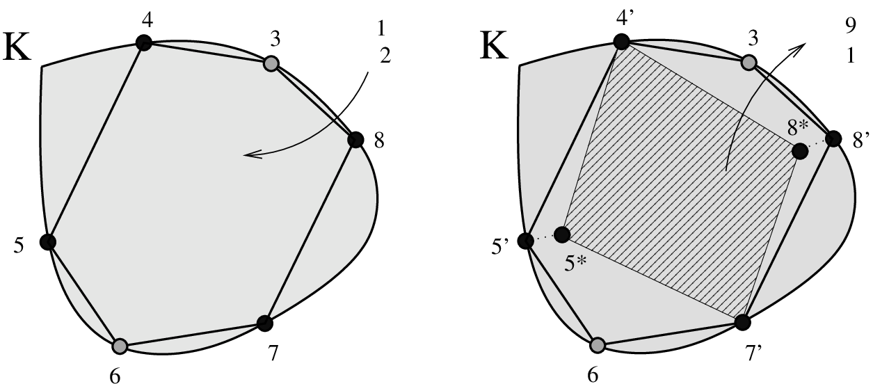
Now we are ready to follow the general induction step from to . Suppose we have defined the sequence of potentials satisfying (1),(2),(3). Here is constant on cylinders of size . We introduce a new set of points on the boundary of . For each denote by the point located exactly along the boundary to the left of and by the point of the same distance to the right. Then the set gives equidistant points on the boundary of . We enumerate these points starting from and moving to the right along the boundary: and so on. The general formula is
| (29) |
We denote the original cylinders of step by . Then for the corresponding point on the boundary of . Furthermore, let be the orbit with the same generator as and , where is a -invariant measure supported on .
We construct the original cylinders of step by replicating the generator of each original cylinder of the previous step times and then changing the last entry to be either 0 or 1. E.g. for define
| (30) |
where is a binary complement to the last entry of . Then the sequence of -tuples and will be the generators of the original cylinders of step . For each cylinder of step we obtain 2 new original cylinders of step . Let . We define as follows
By definition, is constant on cylinders of length and therefore it is continuous on .
Note that and have the same first entrees and different -th entree. Therefore, these elements are mapped into consecutive points under . Since , either or . (Here additive operations on j are performed modulo ).
Now we will estimate . First, suppose for some between 0 and and between 1 and . Then and .
If is odd, then for and hence
| (31) |
If is even, then for . Therefore for (here ) and for . Then the same values repeat periodically for on each of the intervals of length , that is,
where . In this case either or . Summarizing the above we get
Since the distance along the boundary between and is ,
. Also,
The estimates are similar when . In this case, since and differ only by entry, . Thus, . By replacing by in the arguments above we obtain
Finally, consider when . As discussed before, either or . We assume , the other case is similar. If is even, is odd and for . Thus for all . If is odd, is even and for . Then for and for . Since
we conclude that
| (32) |
It follows that
| (33) |
On any cylinder of size the potential is equal to one of the points on the boundary of that were obtained during this or one of the previous steps. Since these cylinders form a disjoint partition of , for any probability measure the rotation vector is a convex combination of the boundary points of . Convexity of implies that .
As before, we denote the original cylinders of step by . Then for let be the corresponding point on the boundary of , be the orbit with the same generator as and , where is a -invariant measure supported on . Since are rotation vectors of and the rotation set is convex, .
Using the fact that for all , we compute
| (34) |
If is odd, for . Then for all and hence . If is even, for . Then for and for . Then is either or for . Assuming we get
| (35) |
Hence,
This proves (3), and the induction is complete.
It follows from (1) and (2) that the sequence converges uniformly to a continuous potential . For any there is such that whenever . Then for and we have
| (36) |
Moreover, for and we have
| (37) |
Therefore, the Hausdorff distance for all and hence converges to .
On the other hand, and the polygons converge to with respect to the Hausdorff metric. Thus, also converges to as . We obtain , which concludes the proof of the theorem.
∎
Remarks.
(i)
The potential obtained in Theorem 1 is not Hölder continuous. To see this, consider and which is a periodic point generated by a -tuple . Then is the point located along to the left of . Point is found by starting at , then moving to the left and to the right along . Then the distance between and decreases as , however where .
(ii)
While Theorem 1 is formulated for a one-sided full shift, the procedure of the proof can be easily generalized to (one and two-sided) shifts and topologically mixing subshifts of finite type.
In case of a topologically mixing subshift of finite type the fact that has positive topological entropy guarantees that has sufficiently many periodical points that can be used to construct the
sequence of potentials converging to a potential and satisfying similar conditions as (1), (2), (3).
We now generalize Theorem 1 to .
Theorem 2.
Let be a compact convex subset of . Then there exist a full one-sided shift map with finite alphabet and a continuous potential such that .
Proof.
We can assume that has non-empty interior, since otherwise we can repeat the argument of the proof in a lower dimension. First note that any open bounded convex set in has Lipschitz boundary ([8, Corollary 1.2.2.3]). Then there is a finite covering of the boundary of by open balls with centers at points of radii and bijective maps from each neighborhood into the unit ball of such that
- (1)
and are Lipschitz continuous with constant .
- (2)
- (3)
For convenience we endow with the maximums norm. Let be a one-sided shift space with alphabet . For each coordinate , we apply the procedure used in the proof of the previous theorem to the interval instead of the boundary curve. Then the functions map each point in into points on the boundary of . To compensate, the potentials will map the cylinders whose generators have only entries from a subset of the alphabet into the points in .
Suppose is any integer between 1 and . We place two initial points in with coordinates and . The original cylinders of step zero will be and and we set , . The original cylinders of step one are constructed in the same way as above using elements and instead of 0 and 1. To select the points in for this step we use the second coordinate and move to the ”left” (negative direction of the -axis) and to the ”right” (positive direction) by . We obtain the following set of points in : , , , . Potential is defined as in (26):
Then we repeat the process with the next coordinate and use the original cylinders of step two to define . After we are finished with coordinate we start again with , but now we shift to the left and right by an additional . Since the number of points in will double each time, we can use the original cylinders of the next step to define the next potential in the sequence. As in the proof of the previous theorem, we obtain a sequence of continuous potentials such that
| (38) |
This estimate is true only for the subsequence since we need steps to reduce the distance between points in in half. We have also adjusted the quantity on the right hand side of condition (2) of Theorem 1. One change is the introduction of the Lipschitz constant . The other change is that the length of the interval [-1,1] is two in contrast to the previous theorem, where we assumed a boundary of length one. The set of points
| (39) |
forms an - net on the boundary of . The corresponding points
in satisfy condition (3) of Theorem 1 up to the constant on the right hand side of the inequality. Thus, the subsequence converges uniformly to a continuous potential and
∎
4. Entropy of rotation sets
In this section we give an alternative definition for rotation sets and its associated entropy function which is more related to the traditional definition of topological entropy and does not make use of the variational principle.
Let be a compact metric space, and let be continuous. Let be a continuous (dimensional) potential. For and we define the -dimensional Birkhoff average at of length with respect to defined by
| (40) |
where . Moreover, we define
| (41) |
Here denotes the open Euclidean ball with center with radius . We frequently write when it is clear to which dynamical system we refer too. Recall the definition of the rotation set , see (2). We define
| (42) |
We have the following.
Proposition 2.
Let be a continuous map on a compact metric space and let be continuous. Then
| (43) |
Proof.
Let and . Define . By Birkhoff’s Ergodic Theorem, the basin of
| (44) |
is a set of full -measure, i.e. . By weak convergence, for all there exists such that for all .
This proves the left-hand side inclusion in (43).
To prove the right-hand side inclusion in (43) let and consider sequences and such that
. The existence of these sequences follows from the definition of .
Define probability measures
Hence . Note that is in general not an invariant measure.
Since the space
of all Borel probability measures on is compact, there exists a Borel probability measure on which is a weak accumulation point of the measures .
It now follows from similar arguments as in the proof of the Krylov-Bogolyubov Theorem (see for example [14]) that is invariant. Moreover, by construction . This completes the proof.
∎
Proposition 3.
Let be a continuous map on a compact metric space and let be continuous. Then
- (i)
Both, and are compact and is convex;
- (ii)
If for all and all exists such that then . In particular, if then .
Proof.
As stated before, the weak compactness and convexity of implies that is compact and convex.
The statement that is closed follows directly from the definition. This proves (i).
Suppose for all and all exists such that . Then , and therefore (ii) is a consequence of (43) and (i).
∎
Remark. As a consequence of Proposition 3 (ii)
we obtain that for topological mixing subshifts of finite type, Axiom A basic sets and expansive systems with specification since in these cases
holds.
The following examples show that both of the inclusions (43) can be strict.
Example 1.
Let with . Let and be continuous with and . Moreover, we assume that and . Consider the potential . The fact that and are both invariant sets of implies that . On the other hand, since the convexity of implies . In particular, the inclusion is strict.
Example 2.
Let be even and let be the one-sided full shift on the alphabet . Let be a compact and convex subset of whose boundary is a closed polygon with vertices which we label counter clock-wise. Since there are at least vertices the set has non-empty interior. Pick in the interior of . Let be the line segments joining and endowed with the canonical order induced by . For each we pick a strictly increasing sequence with , in particular . We also write .
Next, we define several subsets of .
Let and fix .
For all and all we define . Moreover, let .
Finally, we define a potential by
| (45) |
Note that if and only if for all , in particular is conjugate to a full shift in symbols.

We now list several properties of the system in example 2.
Theorem 3.
Let and be as in example . Then
- (i)
is Lipschitz continuous;
- (ii)
;
- (iii)
;
- (iv)
, in particular
and therefore the inclusion is strict;
- (v)
and .
Proof.
(i) We will work with the metric (see (14)) on to show that is Lipschitz continuous. Set . Let with . If then for some . Hence,
| (46) |
The case is analogous. The case and with can be treated analogously as in (46). It remains to consider the case for some . Without loss of generality we assume (with respect the canonical order on . Thus, where is defined by . Since for all we conclude that
| (47) |
which completes the proof of (i).
(ii) Since and since is compact and convex, it follows that . We have . This follows from the fact that for each there exists a fixed point
with . Using that are the extreme points of and that is compact and convex the inclusion follows from the Krein-Milman theorem.
(iii)
By a result Sigmund (see [4]) applied to one-sided full shifts the set of periodic point measures (see (5) for the definition) is weak dense in . Therefore, (iii) follows from Proposition
3 (ii).
(iv) We already have shown in the proof of (ii) that . The statement will be proven in Corollary 1
by using the thermodynamic formalism. Consider . To prove (iv) we have to show that . Let such that lies on the interior of the line segment joining and . By construction of the line segment is a face of and since each invariant measure with must put positive measure on each of the -invariant sets and . This implies that
is not ergodic.
(v) Clearly, for all . Let now . It follows
from a similar argument as in the proof of (iv) that each with must be a convex combination of invariant measures both of which have rotation vectors
in . Therefore, follows from the fact that the measure-theoretic entropy is affine.
Next, we consider . Let be the unique measure of maximal entropy of , i.e., the unique invariant measure satisfying . It follows from the construction
that . Therefore, it suffices to consider .
Let be the unique point on such that lies on the interior of the line segment . Let such that
and . Let such that for we have . Since the measure-theoretic entropy is affine we conclude that .
Finally, follows from the continuity of and from the fact that is connected.
∎
Remark. By property (v), the entropy is on the boundary of strictly smaller than in the interior of . This is however in general not true. Indeed, by slightly modifying
example and concentrating a shift with more then symbols on one of the points , the continuity of implies that .
Next, we introduce an alternative definition for a entropy function which is closely related to the traditional definition of topological entropy.
Recall the definition of the topological entropy of (see (8)),
| (48) |
where is a maximal -separated set. The topological entropy satisfies the variational principle (which is a special case of the variational principle for the topological pressure (9)):
| (49) |
Furthermore, the supremum in (49) can be replaced by the supremum taken only over all . We denote by the set of all measures of maximal entropy, that is the set of measures which attain the supremum in (9). In general may be empty (see for example [20]).
Fix . Let and . We say is a -set if is -separated and for all . For all and we pick a maximal (with respect to the inclusion) -set and define
| (50) |
and
| (51) |
Analogous as in the case of one can show that does not depend on the choice of the -sets . Clearly, and are bounded above by and therefore finite.
We now review a standard construction of invariant measures with large entropy. Given a finite set we define a probability measure by
| (52) |
Recall that for a Borel map and a Borel measure on the push forward of is defined by .
We will need the following result, which is typically shown by using the Misiurewicz argument when proving the variational principle (see, for example, [14, Section 4.5]).
Lemma 1.
Let be a continuous map on a compact metric space and let . Let be a sequence of -separated sets in , and define the measures
| (53) |
Then there exists a weak accumulation point of the measures and any such accumulation point is invariant and satisfies
| (54) |
The next result establishes an inequality between and .
Proposition 4.
Let be a continuous map on a compact metric space, let be continuous and let . Suppose is continuous at . Then .
Proof.
Note that is well-defined by (43). Let . It follows from the definition of (see (51)) and from the continuity of at that there exists such that for all and all we have
| (55) |
and
| (56) |
Using (55) and the definition of we can pick , and an increasing sequence of positive integers such that
| (57) |
We now apply Lemma 1 to the -separated sets and obtain the existence of with and . It follows that and since was arbitrary the claim follows. ∎
Remark.
In the following we establish under rather mild assumptions the identity of and .
We say a topological space is a Besicovitch space if the Besicovitch covering theorem holds. Next, we give an alternative formulation for the measure-theoretic entropy which is due to Katok. Let be a continuous map on a compact metric space and let . For , and we denote by the minimal number of balls in the metric that cover a set of measure greater or equal than . It is shown in [13] that
| (58) |
Given a continuous potential and we say that is approximated by ergodic measures if there exists such that and as . In this case we have (see Proposition 3 (ii)). Being approximated by ergodic measures occurs for several classes of systems and potentials. For example, we will show in Corollary 1 that if satisfies (STP)and is Hölder continuous then can be approximated by ergodic measures for all . We are now ready to state our main result about the identity of and .
Theorem 4.
Let be a continuous map on a compact metric space that is a Besicovitch space with respect to the induced topology. Let be continuous and let such that is continuous at and is approximated by ergodic measures. Then .
Proof.
The inequality is shown in Proposition 4. To show we only need to consider the case . Let be arbitrary. Pick such that
| (59) |
for all . It therefore suffices to show that there exists such that
| (60) |
for all . By uniform continuity of there exists such that if , and then for all we have
| (61) |
Here denotes the -dimensional Birkhoff average defined in (40). Since is approximated by ergodic measures there exists such that and . Let be fixed. Applying (58) and making smaller if necessary we conclude that
| (62) |
for all . From now we consider a fixed . We define
| (63) |
Since is an increasing sequence of Borel sets whose union is a set of full -measure we conclude that
| (64) |
We denote by the number of Bowen balls determining that have non-empty intersection with . For all sufficiently large these balls, due (63), will cover a set of measure for some . It follows from the fact that (58) also holds for that (62) remains true when we replace by . For let denote the largest integer smaller or equal than . Let be a Besicovitch constant of . Note that this constant can be chosen independently of the metrics since they are decreasing in . It follows from the Besicovitch covering theorem that there exist Bowen balls in the collection of balls determining that are pair-wise disjoint. The centers of these balls form a -separated set which we denote by . It follows from (62) and the construction of the set that
| (65) |
Moreover, since each of the balls defining has non-empty intersection with we obtain from (61) and (63) that for all . Finally, we may conclude from (65) (also using the definition of , see (50)) that which completes the proof of the theorem. ∎
5. Entropy via periodic orbits
In this section we consider smooth non-uniformly expanding systems and show that under certain assumptions on the entropy is entirely determined by the growth rate of those periodic orbits whose rotation vectors are sufficiently close to . Our approach heavily relies on previous work by Gelfert and the second author of this paper [6] about the computation of the topological pressure via periodic orbits. Throughout this section we use the notations from Section 2.5.
Let be a smooth Riemannian manifold and let be a -map. Let be compact locally maximal -invariant set. We consider and simply write instead of . Let be a continuous potential with rotation set . To avoid trivialities we will always assume .
We say that is uniformly approximated by measures in if there exist and such that for all , and as well as as .
We now introduce an entropy-like quantity which is entirely defined by the growth rate of those periodic points that have rotation vectors in a given ball about and have some uniform expansion.
Let and let , . Define
| (66) |
if and
| (67) |
otherwise. Furthermore, we define
| (68) |
We have the following.
Proposition 5.
Let and suppose is uniformly approximated by measures in . Let . Then for all we have
| (69) |
Proof.
If the statement is trivial; therefore, we can assume . Let and let . Since is uniformly approximated by measures in there exists with , and .
It is a consequence of Katok’s theory of approximation of hyperbolic measures by hyperbolic sets in it’s version for non-uniformly expanding maps (see for example [6] and the references therein) that there exists a sequence of measures supported on compact invariant expanding sets such that
| (70) |
in the weak topology and that for all . Furthermore, for each there exist such that is conjugate to the full shift in symbols. For every there is a number such that
| (71) |
for all . Moreover, there exists a number with such that for every with we have . Together we obtain
| (72) |
for every . Let such that is topologically conjugate to the full shift in symbols. Since (see [25, Theorem 9.8]), we may conclude that
It now follows from Proposition 1 and an elementary calculation that
| (73) |
Combining (72) and (73) yields
Recall that by (20) the map is non-decreasing as . Since and can be chosen arbitrarily small the claim follows. ∎
The following Theorem is the main result of this section.
Theorem 5.
Let be a -map, and let be a compact -invariant locally maximal set. Let be continuous and let such that is uniformly approximated by measures in and that is continuous at . Then for all ,
| (74) |
Proof.
The part in (74) already follows from Proposition 5. To prove the opposite inequality pick and . Since the right hand side in the limit in (74) is non-increasing as , it suffices to show that
| (75) |
for some . By continuity of at there exists such that for all . Pick such that
| (76) |
for all . If for all , then and (75) trivially holds. Next we consider the case that for some . We define
It follows from the continuity of the minimums norm of that is a compact invariant uniformly expanding set for .11 1 This implies that limit on the left-hand side of (76) is bounded above by and thus in particular finite. For with we define a measure by
| (77) |
where denotes the delta Dirac measure supported at . Note that every measure defined in (77) belongs to and is in the convex hull of the set . Since is weak compact, there exists a subsequence converging to some measure in the weak topology. It follows that and . Since is uniformly expanding, there exists which is an expansivity constant for . In particular, for every and every the set is -separated. It now follows from Lemma 1 that
| (78) |
Combining this with (76) gives (75) and the proof is complete. ∎
Remarks.
(i) While Theorem 5 is stated in the context of non-uniformly expanding systems the analogous result holds for non-uniformly hyperbolic diffeomorphisms of saddle type. For such a map one defines as the
smallest absolute value of the Lyapunov exponents of . We refer to [5] for more details about these classes of systems.
(ii) We recall that the continuity of holds for all
if the entropy map is upper-semi continuous (and therefore particular if is expansive).
(iii) If is a topological mixing hyperbolic set (uniformly expanding or of saddle type) then it can be shown that Theorem 5 holds for all Hölder continuous potentials and all .
Similar results hold for topological mixing subshifts of finite type and expansive homeomorphisms with specification.
(iv) Theorem 5 even provides new information in the case when is a topological mixing hyperbolic set and is the rotation vector of the measure of maximal entropy. Indeed, Proposition 1 provides a version of (74) by considering all periodic points. On the other hand, our result shows that it is already sufficient to consider periodic points with sufficiently “large” Lyapunov exponents and rotation vectors sufficiently close to .
6. Dependence on parameters
Let be a continuous map on a compact metric space. In this section we assume that has strong thermodynamic properties (STP). Let , where for some fixed .
The main goal of this section is to study the dependence of the entropy on in the interior of the rotation set. Recall that since the entropy map is upper semi-continuous (property (2) in the definition of (STP)) it follows that is continuous. Here we show that under the assumption of strong thermodynamic properties is even real analytic on the interior of . We start by introducing some notation.
Given we consider the linear combination of the potentials . We write
| (79) |
It follows from property 3 of (STP) that is a real-analytic function of . Let denote the unique equilibrium measure of the potential (which is well-defined by property 4 of (STP)). As a consequence of (12) we obtain that
| (80) |
Hence, the map is also real-analytic. Writing gives
| (81) |
which implies that is also real-analytic. First we apply results in [10] to obtain a characterization for having non-empty interior.
Proposition 6.
The following are equivalent.
- (i)
No non-trivial linear combination of is cohomologous to a constant.
- (ii)
.
Proof.
Assume that non-trivial linear combination of is cohomologous to a constant. It follows from (13) that is a strictly convex function in .
Therefore, [10, Corollary 3] implies that and thus (ii) holds.
Next, we assume that there exists a nontrivial linear combination of that is cohomologous to a constant. It is easy to see that in this case must be contained in some
lower-dimensional affine subspace of . Since (see [10, Theorem 1]), we conclude that has empty interior.
∎
A side product of the proof of Proposition 6 is the following.
Corollary 1.
If then . In particular, is well approximated by ergodic measures for all .
Next we show that unless has zero topological entropy the map is strictly positive on the interior of the rotation set.
Theorem 6.
Let be a continuous map on a compact metric space satisfying (STP)and let be Hölder continuous. Then one and only one of the following conditions holds.
- (i)
.
- (ii)
for all .
Proof.
Assume . If then (ii) trivially holds. From now on we assume that and thus, by Proposition 6 no nontrivial linear combination of is cohomologous to a constant. Let . As a consequence of Corollary 1 there exists such that . By definition, is the unique equilibrium measure of which implies that .
If , then is the unique measure of maximal entropy and we obtain . Otherwise, there exists with
| (82) |
It follows from Corollary 1 that there exists such that . Applying the variational principle and the fact that is the unique equilibrium measure of the potential yields
| (83) |
∎
Finally we present the main result of this section.
Theorem 7.
Let be a continuous map on a compact metric space satisfying (STP)and let be Hölder continuous. Then is real-analytic on .
Proof.
If is empty there is nothing to prove. From now on we assume . Without loss of generality we only consider the case (i.e. ) and leave the general case to the reader.
Recall that
| (84) |
is a real-analytic surjective map. We will show that is a -diffeomorphism.
Let with .
Combining that and are the unique equilibrium measures of the potentials
and respectively, with (81) implies . We conclude that which implies that
is cohomologous to a constant. Therefore, and we have shown that is a bijection.
Finally, we have to prove that is a local -diffeomorphism.
Equations (13) and (80) combined with the fact that neither nor are cohomologous to a constant imply
that
| (85) |
Consider now the bilinear form
Then coincides with
where
Since no nontrivial linear combination of and is cohomologous to a constant, if then (see [24]) and hence is positive definite. In particular is positive. Using that is the derivative of , implies that for all . It now follows from the inverse function theorem that is a -diffeomorphism. Since is real-analytic we conclude that
is real-analytic in .
∎
We say a sequence of compact sets is a real-analytic exhaustion of if for all , and each is a real-analytic -dimensional submanifold of . The following is a direct consequence of the proof of Theorem 7.
Corollary 2.
Let be a continuous map on a compact metric space satisfying (STP)and let be Hölder continuous with Let is a real-analytic exhaustion of . Then is a sequence of -dimensional real-analytic submanifolds that converges to in the Hausdorff metric. Moreover, varies real-analytically on for all .
References
- [1] T. Bousch, Le poisson n’a pas d’aretes, Annales de l’Institut Henri Poincaré (probabilités et statistiques) 36 (2000), 489-508.
- [2] R. Bowen, Equilibrium states and the ergodic theory of Anosov diffeomorphisms, Lecture Notes in Math. 470, Springer-Verlag, Berlin, 1975.
- [3] R. Bowen, Some systems with unique equilibrium states, Math. Systems Theory 8 (1974/75), 193–-202.
- [4] M. Denker, C. Grillenberger, K. Sigmund, Ergodic theory on compact spaces, Lecture Notes in Mathematics, Vol. 527. Springer-Verlag, Berlin-New York, 1976. iv+360 pp.
- [5] K. Gelfert and C. Wolf, Topological pressure via periodic points, Trans. Amer. Math. Soc. 360 (2008), 545-561.
- [6] K. Gelfert and C. Wolf, On the distribution of periodic orbits, Discrete Contin. Dyn. Syst. 26 (2010), 949–966.
- [7] W. Geller and M. Misiurewicz, Rotation and entropy, Trans. Amer. Math. Soc., 351 (1999), 2927-2948.
- [8] P. Grisvard, Elliptic problems in nonsmooth domains, Monographs and Studies in Mathematics vol. 24, Pitman (Advanced Publishing Program), Boston, MA, 1985
- [9] N. Haydn and D. Ruelle, Equivalence of Gibbs and equilibrium states for homeomorphisms satisfying expansiveness and specification, Comm. Math. Phys. 148 (1992), 155–-167.
- [10] O. Jenkinson, Rotation, entropy, and equilibrium states, Trans. Amer. Math. Soc. 353 (2001), 3713-3739.
- [11] O. Jenkinson, Geometric Barycentres of Invariant Measures for Circle Maps, Ergodic Theory and Dynamical Systems 21 (2001), 511–532.
- [12] O. Jenkinson, Frequency locking on the Boundary of the Barycentre Set, Experimental Mathematics 9 (2000), 309–317.
- [13] A. Katok, Lyapunov exponents, entropy and periodic orbits for diffeomorphisms, Publ. Math., Inst. Hautes Étud. Sci. 51 (1980), 137–173.
- [14] A. Katok and B. Hasselblatt, Introduction to the modern theory of dynamical systems. With a supplementary chapter by Katok and Leonardo Mendoza, Encyclopedia of Mathematics and its Applications, 54, Cambridge University Press, Cambridge, 1995.
- [15] S. Kim, R. S. MacKay and J. Guckenheimer, Resonance regions for families of torus maps, Nonlinearity 2, (1989), 391-404.
- [16] J. Kwapisz, Every convex polygon with rational vertices is a rotation set, Ergodic Theory and Dynamical Systems 12 (1992), 333–339.
- [17] J. Kwapisz, A toral diffeomorphism with a nonpolygonal ratation set, Nonlinearity 8, (1995), 461-476.
- [18] J. Kwapisz, A priori degeneracy of one-dimensional rotation sets for periodic point free torus maps, Trans. Amer. Math. Soc. 354 (2002), 2865-2895
- [19] M. Misiurewicz, Rotation Theory, Misiurewicz’s webpage.
- [20] M. Misiurewicz, Diffeomorphism without any measure with maximal entropy, Bull. Acad. Polon. Sci., Ser. sci. math., astr. et phys, 21 (1973), 903-910.
- [21] M. Misiurewicz and K. Ziemian, Rotation sets and ergodic measures for torus homeomorphisms, Fundam. Math. 137 (1991), 45–52.
- [22] S. Newhouse, Continuity properties of entropy, Ann. of Math. (2) 129 (1989), 215–235.
- [23] H. Poincaré, Sur les cousbes définies par les équations différentielles, Euvres Complètes, tome 1, Gauthier-Villars, Paris, (1952), 137-158.
- [24] D. Ruelle, Thermodynamic Formalism, Cambridge: Cambridge Univ. Press, 2004.
- [25] P. Walters, An introduction to ergodic theory, Graduate Texts in Mathematics 79, Springer, 1981.
- [26] K. Ziemian, Rotation sets for subshifts of finite type, Fund. Math. 146 (1995), 189-201.