Real time assimilation of HF radar currents into a coastal ocean model
Abstract
A real time assimilation and forecasting system for coastal currents is presented. The purpose of the system is to deliver current analyses and forecasts based on assimilation of high frequency radar surface current measurements. The local Vessel Traffic Service monitoring the ship traffic to two oil terminals on the coast of Norway received the analyses and forecasts in real time.
A new assimilation method based on optimal interpolation is presented where spatial covariances derived from an ocean model are used instead of simplified mathematical formulations. An array of high frequency radar antennae provide the current measurements. A suite of nested ocean models comprise the model system. The observing system is found to yield good analyses and short range forecasts that are significantly improved compared to a model twin without assimilation. The system is fast, analysis and six hour forecasts are ready at the Vessel Traffic Service 45 minutes after acquisition of radar measurements.
Subject keywords: data assimilation, ocean modelling, current sensors, ocean
currents.
Regional terms: Europe, Norway, Bergen, Fedje. Bounding coordinates:
( E, N), ( E, N).
Journal of Marine Systems, 28 (3–4), pp 161–182,
doi:10.1016/S0924-7963(01)00002-1.
1 Introduction
Operational forecasting of the oceans is still in its infancy. Unlike the atmospheric weather, ocean currents do not pose an immediate threat to everyday life. Our daily goings-on may indeed never be affected by the strength of the ocean currents in nearby waters. This explains in part why forecasting the state of the atmosphere was a science and a craft as early as in the 1920s while at the turn of the millenium the same can still not be said about the oceans. (See the account of the first, failed attempt at numerically forecasting the atmosphere in Richardson, (1922).)
Another reason for this disparity may be the general impression that the ocean is not as capricious as the atmosphere. While this may be true on some time scales and in some regions, it is certainly not true for the swift coastal surface currents that feed on the contrast in temperature and salinity between neighbouring water masses. When such baroclinic currents are further enforced by the wind field and join up with the tidal motion, the result can be surface currents up to 2 m/s (4 knots) that loosely follow the coastline. These currents vary in width and strength and can quickly break into whorls and eddies of various sizes (typically less than 80 km, see Johannessen et al.., (1989) and Ikeda et al.., (1989)). Such a chaotic dynamical system is unpredictable over longer periods, hence data assimilation of observations is vital when trying to forecast coastal currents.
The complexity of coastal current fields tells us that the pertinent horizontal length scale of ocean dynamics, the Rossby radius of deformation (see Gill, (1982)), which in turn dictates the required horizontal resolution of the numerical models, is vastly different from that of the atmosphere. In the atmosphere, this scale determines the horizontal extent of low and high pressure systems (the good and the bad weather), which is in the range of several hundred kilometers. The equivalent scale in the ocean is only a few tens of kilometers. Hence, resolving eddies in ocean models is only done at an enormous computational cost which seriously limits the horizontal extent of the model domain.
When trying to forecast coastal currents with the aid of data assimilation, the Rossby length scale becomes an acute problem. In weather forecasting, observations of the density field are made with a dense network of radio soundings that resolves the vertical structure of the atmospheric fronts. The density fronts associated with a mesoscale ocean cyclone may be less than a kilometer in horizontal extent. Hence, to achieve the same forecast skill for mesoscale activity in the ocean as in the atmosphere, the vertical and horizontal density structure of the ocean eddies and their associated fronts must be resolved using an extremely dense network of vertical density profilers. Although technically possible (using salinity-temperature-depth meters, CTD, or expendable bathythermographs, XBT), it is neither financially nor operationally feasible to build such a dense coastal real time observation network.
We see that there are numerical, instrumental, and socioeconomic reasons why operational forecasting of the coastal ocean is lagging behind its atmospheric counterpart. However, the appearance of huge oil tankers has caused currents to become a factor to reckon. A tanker moves almost unaffected through bad weather and rough seas, but coastal currents can seriously deflect its bearing. While aiming toward narrow sounds, or maneuvering through channels and straits, it is imperative to know the strength and direction of the currents. Fortunately, there is now a growing awareness of the threat that coastal currents pose to ship traffic and the ensuing pollution and potential loss of lives that such disasters may cause.
There exists however an inexpensive alternative to in situ sampling of oceanographic data. Shore based high frequency (HF) radars provide high resolution surface current coverage in near real time on an extensive observation grid at a very low cost. Although surface currents do not provide a complete picture of a coastal current, it does provide valuable information on its extent, direction, and magnitude. Using HF radars to map coastal currents is by now a well tested technique (see Barrick et al.., (1977) and Barrick, (1978) for early accounts of the methodology) which has matured over the years into reliable instruments.
One of the aims of the project EuroROSE (European Radar Ocean Sensing) is to combine real time radar observations of surface currents with a suite of ocean forecast models using an assimilation scheme to deliver real time analyses and forecasts of coastal currents to the Vessel Traffic Services (VTS) in dangerous regions with extensive ship traffic. The net site http://ifmaxp1.ifm.uni-hamburg.de/EuroROSE provides more information on the project as a whole.
Assimilating HF radar surface currents into models of the coastal ocean is a relatively new approach to improving coastal current forecasts. The authors are only aware of two other similar efforts. Oke et al.. ((2002)) describes a data assimilation system which utilizes a CODAR HF radar (see Barrick et al.., (1977) for a description of an early version of the radar) and the Princeton Ocean Model to produce forecasts of the wind-driven, mesoscale shelf circulation off the Oregon coast. The results are promising, including the vertical impact of the surface currents. However, this system is only used for hindcast studies. The Rutgers University has an ongoing assimilation effort associated with their underwater laboratory LEO-15 Glenn et al.. ((2000)) off the coast of New Jersey. During five week campaigns in the summer months, they perform real time assimilation of CODAR radar data into their Regional Ocean Model System (ROMS, see Song & Haidvogel, (1994) for a description of an early version of the model) and produce forecasts of coastal currents. More details of the system can be found at http://marine.rutgers.edu/mrs/.
The first realization of the EuroROSE observing system was focussed on the island Fedje off the west coast of Norway. This area is bustling with tankers and other ships that serve the petroleum terminals Sture and Mongstad, together one of the busiest petroleum harbours in the world. The ship entrances are narrow and the coastal current is strong and rapidly changing in location and direction. Fig 1 provides an overview of the area and typical radar coverage during the experiment.


As the main objective of the project was to demonstrate the potential of such an ocean monitoring and forecasting system for coastal security, the information was transmitted in real time to the local vessel traffic service (VTS) where observations, analyses, and forecasts were presented automatically.
In this paper, we present the theory behind the assimilation scheme together with its implementation and performance in the real time monitoring and forecasting system which was developed for the region around Fedje. The radar system and the numerical model are also described in some detail.
2 Sequential data assimilation
Data assimilation methods have been used routinely by the major weather prediction centres for the past two decades Daley ((1991)). These methods vary in complexity from simple Newtonian nudging schemes through optimal interpolation schemes and all the way up to four dimensional variational assimilation schemes and sequential Kalman filtering techniques. The latter method has also been demonstrated for simplified models (the Lorenz equations and quasi geostrophic models, see Evensen, (1994); Evensen, (1997)).
The fundamental equation in sequential data assimilation is
| (1) |
Here, is the -dimensional model state vector, with superscripts “a” and “f” denoting analysis and forecast. Further, is the gain matrix, and is the data vector (the observations). Finally, is the observation operator which maps the model state onto the observation space.
As an explanation to the observation operator, consider a 3D ocean model yielding horizontal current vectors at certain vertical levels. The data provided are surface currents measured with a radar facility. Unless the model and the radar yield data in the exact same locations, some kind of interpolation is needed to make modelled and observed fields comparable.
The gain is a matrix of weights that determines each observation’s influence on the final analysis. Using a minimum variance principle (see Daley, (1991)), we can argue that should be
| (2) |
where is the error variance-covariance matrix of the numerical model, and is the error variance-covariance matrix of the observations.
Let indices and denote model variables and and denote observations, i.e., , and . The model state vector mapped to observation space can then be written
and the model error variance-covariance matrix is
| (3) |
Here and throughout, primes indicate zero-mean quantities (deviations from the mean).
The gain matrix in Eq (2) can be made more understandable by first noting that
is simply the error covariance between model variable and observation . Secondly, the purpose of the inverse weight matrix in Eq (2) is to weight observations according to their importance. Hence, in a cluster of observations, one more data point will normally not add much information as the internal correlation between the observations will be high. Conversely, a solitary observation in a critical location may be heavily weighted. The inverse weight matrix achieves this by balancing the error covariances between observation locations and as predicted by the numerical model,
against the “instrumental” quality of the observations and their internal covariance, which is contained in the observation error variance-covariance matrix,
| (4) |
2.1 Statistical (optimal) interpolation
Statistical or optimal interpolation (OI) is a sequential data assimilation method using predefined (time invariant) error statistics. Hence, the assimilation (analysis) is variance minimizing only if the error statistics are correct and do not change with time (see Daley, (1991)).
OI schemes normally assume either that correlations between two variables and , say, in different locations are functions of distance and direction,
or even isotropic functions of distance only,
Here, is the radial distance and is the direction from to relative to north. These simplifications can sometimes be adequate, but if the covariances display a more complex spatial structure then this formulation may lead to serious errors in the assimilation update.
2.2 The Ensemble Kalman filter
A much more advanced sequential method is the so called Ensemble Kalman filter (EnKF, see Evensen, (1994), Evensen, (1997), and Burgers et al.., (1998)). The method is based on the Kalman filter approach, but circumvents the closure problem of nonlinearity in the model by calculating the covariances from an ensemble of evolving model states. This approach also avoids forecasting the covariance matrix which becomes intractable for 3D oceanic and atmospheric models of realistic dimensions.
An ensemble of initial model states
is generated and integrated forward in time, yielding an ensemble of forecasts at a later time ,
The ensemble average is
| (5) |
and the deviations from the mean are denoted .
The zero mean ensemble can also be viewed as a collection of column vectors, illustrated by the following tableau,
| (6) |
The model error covariance matrix can be approximated by the outer product of the ensemble,
| (7) |
At each update, the Kalman gain must be found from Eq (2) by first integrating numerical model realizations (where is typically ) and then computing using Eq (7). Clearly, this method is computationally very expensive, and it would be desirable to find a middle ground between the over-simplification of standard OI and the enormous cost of running sibling models.
2.3 A “quasi-ensemble” assimilation scheme
We propose to exchange the ensemble of models used to compute the Ensemble Kalman Filter with an ensemble of model states. This can be any collection of model states taken from a representative model run. Whereas an ensemble of models will pick up periods of high and low variance, our covariances will remain fixed throughout the assimilation period. This means that an assimilation scheme employing these statistics will formally belong to the class of previously discussed optimal interpolation schemes.
In order to generate this quasi ensemble, we need to run the model for a representative period. Model states are sampled from the model run. This reference period should be selected carefully. Ideally, it should pick up the correlations relevant for our specific time period. However, this may be impossible to do in advance, as is the case for a real time observing system. For a hindcast experiment, one should naturally choose the reference run to cover the period of interest. The next best thing will be to choose a reference run that covers a similar period (similar climatology, e.g., a different year but same time of year).
A final caveat regarding the sampling is to choose a sampling frequency that captures the relevant physics. This is especially critical for the tidal motion with its well-defined frequencies. This is most easily achieved by choosing a sampling period that is smaller than the dominant tidal period, but not an integer fraction of it (to avoid capturing only high tides or only low tides).
An EnKF will find the “correct” error statistics under the assumptions that the ensemble is sufficiently large and the errors are normally distributed. The proposed quasi ensemble will not, in general, find the correct error variances for the model since its statistics do not vary with time. However, the correlations may be satisfactory. This means that although the relative weight between data and model may be off, the spatial correlations between, say, surface currents in one point and the salinity in another point, may be quite all right.
The formulation of the quasi-ensemble filter is analogous to the derivation of the EnKF and makes no assumptions on the spatial shape of the covariances. In theory, cross-correlations between all pertinent model variables may be used to make full use of the data, hence model grid points well outside the area covered by observations may experience corrections based on their covariance with variables in points closer to the observations. Likewise, vertical corrections can be made to the different model variables. The full equation reads
| (8) |
Here, we have substituted the ensemble (of sampled model states) for using Eq (7).
3 The EuroROSE current assimilation and forecasting system
3.1 The numerical model
We used the Princeton Ocean Model (POM) as implemented and modified by The Norwegian Meteorological Institute (DNMI). The lateral hydrodynamic equations are solved on an Arakawa C-grid (see Mesinger & Arakawa, (1976), Kowalik & Murty, (1993) p 170). Terrain following -coordinates resolve the vertical, which means that the vertical resolution is high in shallow areas and coarse in deeper areas. In addition, the levels are not distributed linearly over the depth as the mixed layer near the surface requires higher resolution than the deeper parts of the ocean. Surface elevation and the vertical component of the current vector, , are solved on the surface. Through the water column, and are staggered one half grid cell with respect to . Hence, the horizontal velocities of the uppermost layer are found one half grid cell from the surface.
The model contains a second-order moment turbulence closure sub-model Mellor & Yamada ((1982)) which provides vertical mixing coefficients. The model solves the conservation equations for momentum and mass using an explicit finite difference scheme in the horizontal, and an implicit scheme for the vertical terms to eliminate the time-step constraints caused by fine resolution of the surface layer. The model has a free surface and uses mode-splitting for the time-stepping. In the external mode, the model is two-dimensional and uses a time-step limited by the Courant-Friedrichs-Lewy (CFL) criterion for fast propagating barotropic waves. For the internal mode, the model is three-dimensional and uses a longer time-step based on the CFL-criterion for internal wave speed. A Leapfrog scheme is used for the advection terms. The model version developed at DNMI has a Flow Relaxation Scheme (FRS) implemented at the lateral open boundaries Martinsen & Engedahl ((1987)), where forcing from eight tidal constituents is also included Engedahl ((1995)). A thorough description of the basic model setup can be found in Blumberg & Mellor ((1987)). For further information on the modifications made to the DNMI version of the model please refer to Engedahl ((1995)).
3.1.1 The model realization
Three models are nested inside each other. The outer model covers the North Atlantic and the Norwegian sea with a resolution of approximately 20 km. The intermediate model covers the coastal waters of southern Norway with a resolution of 4 km (see Fig 2), and the inner, high resolution model has a resolution of 1 km and covers a km area (see Fig 3). The inner model has 17 -levels which are distributed as follows (values are given as parts per thousand of total depth),
| (9) |
The above distribution of -layers is illustrated in Fig 5 with symbols “o” and “x” on the correlation profiles.
The main part of the area covered by the radar antennae has a water depth of m. At this depth, the height of the uppermost grid cell is m (cf Eq (9)). As the horizontal current components are staggered with respect to the vertical component, the uppermost horizontal currents are computed at a depth of m. Measurements made with HF radar are essentially weighted averages of the currents in the vertical column that “feel” the ocean Bragg wave Fernandez et al.. ((1996)). The radar frequency is MHz. Its backscatter is in resonance with an ocean wave of m. The corresponding average current depth is estimated to be m, hence the radar currents are comparable to the currents in the uppermost model layer.
The models are matched using a flow relaxation zone extending seven grid points into the model domain. All three models are run on rotated polar stereographic grids. The topography used in the high resolution model is taken from the ETOPO5 database which is publicly available on the Internet. The dataset is rather too coarse for our application with a resolution of approximately 4.5 km east-west and 9 km north-south. In order to get the entrances between the islands right, we used ship charts to manually correct the topography of the inner model. This explains why Fig 3 exhibits rather more detail in the estuary than along the coast. Tides are included in the intermediate model and are propagated as a barotropic signal into the nested model. No ice model is included, as we are in a permanently ice-free part of the Norwegian Sea. Monthly mean values for river runoff are included in all three models. The wind fields and boundary values are updated every three hours. The outer models are forced with 50 km resolution winds from a limited area atmospheric model (LAM). The inner model is forced using winds from a 10 km resolution atmospheric model to include topographic effects near the coast. Both atmospheric models and the two outer ocean models are run routinely by DNMI.


3.1.2 The model error statistics
As explained in Sec 2.3, the assimilation scheme requires a reference run to compute the model error covariance matrix. In our case, the model period was Feb-Mar 2000, and consequently we ran the model for the same period in 1999 with a sampling period hours, assuming that “on the average” this model run would pick up the important correlations inherent to the model state. The choice of is guided by the observations made in Sec 2.3 that integer multiples of the major tidal constituents should be avoided. A period of 5.5 h will march slowly through the tidal cycle and thus avoid sampling only, say, the high tide and the ebb.
The result of this reference run was then scrutinized and found to yield sensible results. The full correlation matrix of the model can be seen as a six-dimensional object,
| (10) |
where and may assume all model variables in all different grid points in the model domain.
In Fig 4, a slice through the model correlation matrix has been made by freezing at grid point (40,40,1), marked with an “X”. This point was chosen because it lies in the centre of the radar coverage. The model grid orientation is such that is the alongshore current and the across-shore current. The across-shore current correlation shows the expected behaviour of decorrelation with radial distance. Further, the cross correlation between and is found to be quite strong. Its maximum is shifted away from the location X, meaning that the maximum cross correlation does not occur on the spot.


The vertical correlation structure with the surface current in point X(40,40,1) is shown in Fig 5. The model layer depths are indicated with symbols “o” and “x” in the cross correlation with and . As is seen, the model resolves very well the upper 50 m of the ocean. This is necessary to capture the influence of the atmosphere on the oceanic mixed layer. In general, the surface currents do not correlate strongly with the hydrography of the underlying water masses. The strongest correlations are of the order of -0.4.
The across-shore current exhibits a slightly stronger correlation with the hydrography than the alongshore current. Negative correlation indicates that across-shore currents advect fresh and cold coastal waters away from the coast (remember that the location of the point X(40,40) is quite far from shore). The alongshore surface current is completely detached from the hydrography and only at about 50 m depth does the correlation rise above an absolute value of 0.2.
The model statistics reveal a strong surface current to deeper current correlation, but a significantly weaker cross correlation between current components. Note also the immediate drop in correlation at the surface to about 0.8 at 20 m depth. This illustrates how the wind energy is distributed in the upper water column.


3.2 The data
Our observations are taken from a beam forming phased array HF radar called “Wellen Radar” (WERA). The radar is operated by the University of Hamburg and was temporarily mounted on the islands Lyngøy and Fedje. Each radar array measures the radial component of the surface current. For a walk through the theoretical underpinnings of the current measurements, refer to Essen et al.. ((2000)), Gurgel & Antonischki ((1997)) and Gurgel et al.. ((1999)). The radar range is affected by the sea state, atmospheric disturbances, radio interference and sun spot activity. Fig 1 illustrates the variability in radar coverage.
The data are delivered on a regular grid in geographical coordinates (longitude and latitude, see Fig 3). The resolution of this grid is 1 km, which makes the data density comparable to the model grid, albeit with different orientation. Independent measurements of both and can only be found in a triangle covered by both arrays (see Fig 3).
The geometric dilution of precision (GDOP) is the geometric error made when combining two radial current components. This error reaches a maximum when the two radial components are nearly in the same or in opposite directions, see Chapman et al.. ((1997)). The GDOP has been computed for the east and north components of the radar current vectors (see Fig 6). These time-invariant error variances enter the diagonal of the error variance-covariance matrix in Eq (2) to weight observations against the forecast. No information is available on the error covariance between observations, hence is assumed to be diagonal. We have chosen to only include the time-invariant part of the observation error (assuming an RMS error of 5 cm/s on the radial components and then computing the GDOP) to speed up the observing system. To compensate for this procedure, we have included an extra data quality check described in Sec 3.3.1.

3.3 The assimilation cycle
New data arrive every 20 minutes from the radar. Each model cycle consists of assimilation at times -00:40, -00:20, and 00:00 relative to the analysis time. After this, the model generates a six hour forecast (see Table 1 and Fig 7). This cycle is repeated every hour, resulting in several overlapping forecasts. Because we assimilate every 20 minutes, the initial field that starts the next assimilation cycle is a 20 minute forecast based on the assimilation in the previous cycle.
Time [h] Action -1:00 Model is initialized from previous assimilation cycle -0:40 First dataset in, assimilation -0:20 Second dataset in, assimilation 0:00 Third dataset in, final assimilation 0:00 Time of analysis, forecast begins 6:00 Forecast ends

At the outset, it was considered worthwhile to include the cross-correlations between surface currents and hydrography ( and , see Fig 5), both horizontally and vertically. This way the density field could be corrected to make it consistent with the observed velocity field. However, even after smoothing the analysis using a second order Shapiro filter (see Sec 3.3.1), we found the model to go unstable. It turns out that because the model is nested inside an external model that is oblivious of any assimilation, corrections in and cause a density gradient to build up along the open boundary. This sets up an unphysical circulation which eventually blows up the model (see Fig 8 for an example). To save the assimilation experiment, we were forced to leave out cross-updates of hydrography. This limits the memory of the assimilation, as the hydrography is no longer consistently updated with the current field and will cause the current field to lapse back to its original state more quickly. The only solution to the observed mismatch between our nested models is to perform an assimilation in both models (inner and outer). That, however, would be a much more extensive task and was not considered possible in a real time experiment like this. In light of the weak correlations found between surface currents and hydrography (Fig 5) we conclude that in this model realization it is better to leave out corrections to and anyway.

3.3.1 Data quality control and smoothing
To avoid extreme updates in the model due to bad data, a comparison between the modelled and observed currents is made for each observation prior to analysis. If the observed speed differs by more than m/s, or the observed direction deviates by more than from the modelled current vector, the observation is discarded. These thresholds have been chosen rather arbitrarily, but have stood the test and proved to weed out the strong, erroneous current vectors that are often found along the rim of the radar maps (due to backscatter from the strong antenna pattern sidelobes found on the edges of the radar coverage). This quality check is also a way to compensate for the lack of time-varying observation error variances. On the average, only a small percentage of the observations were discarded through this procedure (less than 5%). However, in situations where the radar performed poorly, larger amounts of data were discarded.
Further, the assimilation sometimes adds too much fine structure to the model fields. To remove this but retain the longer wavelengths we chose to run a Shapiro second order nine-point filter after each analysis. It has been shown (see Shapiro, (1970) or Haltiner & Williams, (1980)) that the Shapiro filter removes the “” wave completely (the shortest wave that can be represented, dictated by the Nyquist frequency), while the longer wavelengths are not much dampened (zero damping for infinite wavelength). The “” wave is attenuated by less than 10%.
3.3.2 Restarting the model
The ocean model uses centered differences in space and time (leapfrog scheme) for the integration of the horizontal momentum equations.
As a demonstration of the scheme, we take the one-dimensional advection equation
| (11) |
where is the (constant) advection velocity. Applied to this equation, the leapfrog scheme becomes
| (12) |
Here, is the spatial index and the temporal index. Further, and represent the spatial and temporal resolution, respectively.
The assimilation scheme is invoked at time , which is incompatible with the above scheme because it involves , and hence the corrections introduced by the assimilation would not be propagated forward in time (as the scheme “leapfrogs” past time from time to ). To circumvent this, we have to apply a one level scheme immediately after the update,
| (13) |
This is known as an Euler scheme and is unconditionally unstable for all wavelengths Haltiner & Williams ((1980)). However, the scheme can still be used for a few timesteps at a time as long as we revert to a stable scheme later.
4 Assimilation performance
The observing system was active for a period of approximately six weeks. The assimilation scheme in its final form was used for three weeks. Throughout the experiment, an identical model twin was run without assimilation (hereafter referred to as the free run). This freerunning model allows us to assess the impact of the assimilation scheme on analysis and forecasts. In the following, we have compared the two model runs with the radar data in wont of other sources of ground truth. It is important to keep in mind that the radar data themselves have errors.
For an example of the difference between the free run and the analysis, compare the left and right panels of Fig 14. The free run is clearly less energetic, and the coastal current appears wider and more diffuse than the assimilated current field. Fig 15 shows a close-up of the radar covered area. It is obvious that the assimilation scheme captures the strength and extent of the coastal current very well in this particular instant.
More important than the quality of the analysis itself is the temporal impact of the analysis. I.e., for how long does the added information keep the model forecast on track? To assess this, we computed the spatially averaged kinetic energy in the radar covered area for both model and observations;
| (14) |
where is the area covered by the radar and is the horizontal current speed. The density is assumed constant and left out. This method has the advantage of appreciating a corrected current field (typically the coastal current) even when the current maximum is slightly dislocated by the model yet still improved over the free run.
Fig 9 shows the ratio of the model fields to the observed fields, . As can be seen, the free run underestimates the energy level of the coastal current (roughly by 50%). The analysis is a significant improvement over the free run (same figure), with an energy level on a par with what is observed. After analysis, the forecasts spread out quickly, but retain an average energy level well above that for the freerunning model even after a six hour forecast.
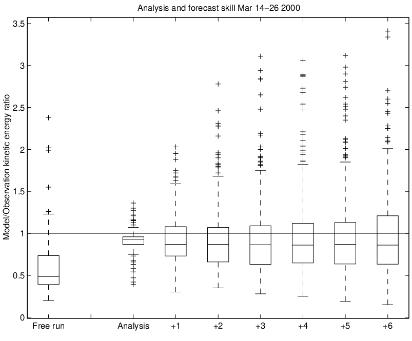
The scatter plot is a more conventional way to compare datasets. Fig 10 shows how the energy level decorrelates as the forecast time increases. At the time of analysis (the assimilation itself), the fields match up almost perfectly. Two hours from analysis, the correlation is still good, but as the boxplots also suggested, there is a lot more spread. Another observation is that the best fit linear regression line dips down compared to the ideal line, which means that the energy level drops off with forecast lead time. Compared to the free run, it seems that forecasts up to three hours correlate better with observations.

The probability distributions of two datasets can be compared with an empirical quantile-quantile plot (EQQ, see Kleiner & Graedel, (1980) or Wilks, (1995)). The cumulative distribution function (CDF) of a dataset is
| (15) |
The CDF is a monotonically increasing function, hence its inverse may be found. The median (mid point) is , the upper quartile is , and so forth. Plotting these values against each other reveal differences in the underlying probability distributions. If a population is a linear transform of , i.e. , the quantiles will fall on a straight line.
Fig 11 shows the QQ-plots of average kinetic energy of the analysis, the +6 hour forecast, and the free run vs radar data. The distribution of the analysis is almost identical to the radar data, with a slope close to unity. The +6 hour forecast has a weaker slope, again suggesting that the forecasts are not able to keep up the coastal current. However, the underlying distribution seems to be of the same form as the radar data. Finally, the free run displays an even weaker energy field and stronger deviations from the radar distribution. All three datasets display some deviations in the upper extreme tail.

Time series of current speed were extracted from the radar data and the model grid point nearest the position . This point was chosen because it is in the central area of interest for the VTS, and always covered by the radar, even in situations with very low radar coverage. Fig 12 shows the correlation between observed and modelled current speed. The freerunning model correlates extremely poorly with observations in this particular point and is clearly not able to capture the intensity of the coastal current.

Finally, the spectral characteristics of the modelled currents were studied. Time series of analysed speed, forecasted speed (at different lead times), and forecasts from the free run were compared to the radar data. The time series were subjected to a coherency analysis. The squared coherency spectrum between two time series is defined as
| (16) |
where and denote the power spectral density (variance spectra) of the observed and modelled time series, and is the complex cross spectral density (see Emery & Thomson, (1997)). Confidence limits based on the number of equivalent degrees of freedom are computed following Thompson ((1979)),
| (17) |
Here, indicates confidence level ( means a 95% confidence interval). The limiting value gives the level up to which squared coherency values may occur by chance Emery & Thomson ((1997)). Fig 13 shows the squared coherency for the analysis, the free run, and forecast lead times +2, +4, and +6 hours. Good coherency is found for the analysis. The coherency then drops regularly with forecast lead time until it becomes barely distinguishable from the free run at six hours from the analysis time. The forecasts cross the confidence limit at approximately five-hourly periods (), hence higher frequencies are not trustworthy. For the free run, a lower sampling frequency was used, leading to a lower cutoff frequency compared to analysis and forecasts in the figure. This lower cutoff also results in a higher (i.e. poorer) confidence level for the free run. For all forecast lead times, we observe a maximum in coherency around the dominant tidal period , indicating that the tidal motion is also improved by the assimilation.
We conclude that lower frequencies corresponding to periods of more than 6 hours are improved by assimilating radar data whereas the higher frequencies are much more difficult to get right. This means that the high frequency features assimilated into the model do not evolve correctly. This seems reasonable, as the low frequencies associated with the slow meandering of the coastal current will be a more persistent feature in the radar data than the swift, smaller scale eddies that move in and out of the radar view.


5 Conclusion
We have demonstrated that it is possible to make real time analyses and forecasts of coastal currents using a suite of nested ocean models and continuous radar coverage. Both analysis and forecasts clearly outperform the free run, indicating that the assimilation has added information to the model, but the +6 hour forecast is only marginally better (if better at all) than the free run. The assimilation scheme also improves the spectral characteristics of the ocean model, especially for frequencies corresponding to periods longer than five hours.
Given the relatively limited coverage of the HF radar, the analyses provide valuable added information through the extrapolation from radar observations to the surrounding waters covered by the model grid.
We were unable to correct the hydrography using the radar currents. This appears to be a fundamental problem with assimilation in nested models. The only way to avoid this will be to do assimilation in both the outer and the inner model. This is a much more time-consuming approach and was not considered feasible in this real time experiment. We also conclude that the relatively weak cross-correlations observed between modelled surface currents and the hydrography discourage this line of approach.
In general, the assimilation scheme is sufficiently sophisticated to allow for long-ranging corrections outside the actual radar coverage (extrapolation), yet fast enough to fit in the tight schedule of a real time framework. The total time from acquisition of data until the presentation of analysis and forecast was ready at the Vessel Traffic Service in Fedje was 45 min. The system was found to be quite robust to bad observations and was able to operate during periods of high and low radar coverage.
Acknowledgements
The authors were funded by the EU MAST-III project “European Radar Ocean Sensing” (EuroROSE), contract no. PL971607. The authors wish to thank Klaus-Werner Gurgel for delivering the radar data and Geir Evensen for discussions on assimilation and diagnosing the results. Thanks also to Heinz Günther for coordinating EuroROSE. The thoughtful reviews by Dr Jun She and one anonymous reviewer are also appreciated.
References
- Barrick ((1978)) Barrick, D.E. (1978). HF Radio Oceanography—A Review. Boundary Layer Meteorol 13 23–43.
- Barrick et al.. ((1977)) Barrick, D.E., Evans, M.W. & Weber, B.L. (1977). Ocean Surface Currents Mapped by Radar. Science 198 138–144.
- Blumberg & Mellor ((1987)) Blumberg, A.F. & Mellor, G.L. (1987). A description of a three-dimensional coastal ocean circulation model. In N.S. Heaps (Ed.), Three-dimensional coastal ocean models. : American Geophysical Union, Washington D C.
- Burgers et al.. ((1998)) Burgers, G., van Leeuwen, P.J. & Evensen, G. (1998). Analysis Scheme in the Ensemble Kalman Filter. Mon Wea Rev 126 1719–1724.
- Chapman et al.. ((1997)) Chapman, R.D., Shay, L.K., Graber, H.C., Edson, J.B., Karachintsev, A., Trump, C.L. et al. (1997). On the accuracy of HF radar surface current measurements: Intercomparisons with ship-based sensors. J Geophys Res 102 C8 18737–18748.
- Daley ((1991)) Daley, R. (1991). Atmospheric Data Analysis ( 2). Cambridge: Cambridge University Press.
- Emery & Thomson ((1997)) Emery, W.J. & Thomson, R.E. (1997). Data analysis methods in physical oceanography. New York: Pergamon Press.
- Engedahl ((1995)) Engedahl, H. (1995). Implementation of the Princeton Ocean Model (POM/ECOM3D) at The Norwegian Meteorological Institute (DNMI) Research Report No. 5. Oslo, Norway: The Norwegian Meteorological Institute.
- Essen et al.. ((2000)) Essen, H-H., Gurgel, K-W. & Schlick, T. (2000). On the accuracy of current measurements by means of HF radar. IEEE J Ocean Eng 25 4 472–480.
- Evensen ((1994)) Evensen, G. (1994). Sequential data assimilation with a nonlinear quasi-geostrophic model using Monte Carlo methods to forecast error statistics. J Geophys Res 99 C5 10143–10162.
- Evensen ((1997)) Evensen, G. (1997). Advanced data assimilation for strongly nonlinear dynamics. Mon Wea Rev 125 1342-1354.
- Fernandez et al.. ((1996)) Fernandez, D.M., Vesecky, J.F. & Teague, C.C. (1996). Measurements of upper ocean surface current shear with high-frequency radar. J Geophys Res 101 C12 28615–28625.
- Gill ((1982)) Gill, A.E. (1982). Atmosphere-Ocean Dynamics ( 30). San Diego, California: Academic Press, Inc.
- Glenn et al.. ((2000)) Glenn, S.M., Boicourt, W., Parker, B. & Dickey, T.D. (2000). Operational Observation Networks for Ports, a Large Estuary and an Open Shelf. Oceanography 13 1 12–23.
- Gurgel & Antonischki ((1997)) Gurgel, K-W. & Antonischki, G. (1997). Measurement of surface current fields with high spatial resolution by the HF radar WERA. In Proceedings of the IGARSS’97 conference ( 1820–1822).
- Gurgel et al.. ((1999)) Gurgel, K-W., Antonischki, G., Essen, H.H. & Schlick, T. (1999). Wellen Radar (WERA): a new ground-wave HF radar for ocean remote sensing. Coastal Engineering 37 3–4 219–234.
- Haltiner & Williams ((1980)) Haltiner, G.J. & Williams, R.T. (1980). Numerical prediction and dynamic meteorology. New York: Wiley and sons.
- Ikeda et al.. ((1989)) Ikeda, M., Johannessen, J.A., Lygre, K. & Sandven, S. (1989). A process study of mesoscale meanders and eddies in the Norwegian Coastal Current. J Phys Oceanogr 19 20–35.
- Johannessen et al.. ((1989)) Johannessen, J.A., Svendsen, E., Sandven, S., Johannessen, O.M. & Lygre, K. (1989). Three-Dimensional Structure of Mesoscale Eddies in the Norwegian Coastal Current. J Phys Oceanogr 19 3–19.
- Kleiner & Graedel ((1980)) Kleiner, B. & Graedel, T.E. (1980). Exploratory Data Analysis in the Geophysical Sciences. Rev Geophys Space Phys 18 699–717.
- Kowalik & Murty ((1993)) Kowalik, Z. & Murty, T.S. (1993). Numerical modeling of ocean dynamics ( 4). New York: World Scientific Publishing.
- Martinsen & Engedahl ((1987)) Martinsen, E.A. & Engedahl, H. (1987). Implementation and Testing of a Lateral Boundary Scheme as an Open Boundary Condition in a Barotropic Ocean Model. Coast Eng 11 603–627.
- Mellor & Yamada ((1982)) Mellor, G.L. & Yamada, T. (1982). Development of a turbulent closure model for geophysical fluid problems. Rev Geophys Space Phys 20 851–875.
- Mesinger & Arakawa ((1976)) Mesinger, F. & Arakawa, A. (1976). Numerical Methods Used in Atmospheric Models GARP Publications Series No. 17. : World Meteorological Organization.
- Oke et al.. ((2002)) Oke, P.R., Allen, J.S., Miller, R.N., Egbert, G.D. & Kosro, P.M. (2002). Assimilation of surface velocity data into a primitive equation coastal ocean model. J Geophys Res 107 C9 3122, 25pp, doi:10.1029/2000JC000511.
- Richardson ((1922)) Richardson, L.F. (1922). Weather Prediction by Numerical Process. Cambridge: Cambridge University Press, reprinted Dover, 1965.
- Shapiro ((1970)) Shapiro, R. (1970). Smoothing, filtering, and boundary effects. Rev Geophys Space Phys 8 359–387.
- Song & Haidvogel ((1994)) Song, Y. & Haidvogel, D.B. (1994). A semi-implicit ocean circulation model using a generalized topography following coordinate system. J Comput Phys 115 228–244.
- Thompson ((1979)) Thompson, R.O.R.Y. (1979). Coherence Significance Levels. J Atmos Sci 36 2020–2021.
- Wilks ((1995)) Wilks, D.S. (1995). Statistical Methods in the Atmospheric Sciences. London: Academic Press.