Computable Carathéodory TheoryThanks: I.B. and M.Y. were partially supported by NSERC Discovery Grants. C.R. was partially supported by project FONDECYT No. 11110226.

Ilia Binder, Cristobal Rojas, Michael Yampolsky

Date: August 24, 2026

Abstract.

Conformal Riemann mapping of the unit disk onto a simply-connected domain $W$ is a central object of study in classical Complex Analysis. The first complete proof of the Riemann Mapping Theorem given by P. Koebe in 1912 is constructive, and theoretical aspects of computing the Riemann map have been extensively studied since. Carathéodory Theory describes the boundary extension of the Riemann map. In this paper we develop its constructive version with explicit complexity bounds.

1. Introduction

Let ${\mathbb{D}}=\{|z|<1\}\subset{\mathbb{C}}$ . The celebrated Riemann Mapping Theorem asserts:

Riemann Mapping Theorem.

Suppose $W\subset{\mathbb{C}}$ is a simply-connected domain in the complex plane, and let $w$ be an arbitrary point in $W$ . Then there exists a unique conformal mapping

f:{\mathbb{D}}\to W,\text{ such that }f(0)=w\text{ and }f^{\prime}(0)>0.

The inverse mapping,

\varphi\equiv f^{-1}:W\to{\mathbb{D}}

is called the Riemann mapping of the domain $W$ with base point $w$ . The first complete proof of Riemann Mapping Theorem, given by P. Koebe in 1912 [12] was constructive. Computation of the mapping $\varphi$ is important for applications, and numerous algorithms have been implemented in practice (see [14, 15]). Theoretical aspects of computing the Riemann mapping were studied exhaustively in [3], where a precise complexity bound on such algorithms was established.

The theory of Carathéodory (see e.g. [18, 19]) deals with the question of extending the map $f$ to the unit circle. It is most widely known in the case when $\partial W$ is a locally connected set. We remind the reader that a Hausdorff topological space $X$ is called locally connected if for every point $x\in X$ and every open set $V\ni x$ there exists a connected set $U\subset V$ such that $x$ lies in the interior of $U$ . Thus, every point $x\in X$ has a basis of connected, but not necessarily open, neighborhoods. This condition is easily shown to be equivalent to the (seemingly stronger) requirement that every point $x\in X$ has a basis of open connected neighborhoods. In its simplest form, Carathéodory Theorem says:

Carathéodory Theorem for locally connected domains.

A conformal mapping $f:{\mathbb{D}}\to W$ continuously extends to the unit circle if and only if $\partial W$ is locally connected.

A natural question from the point of view of Computability Theory is then the following:

Suppose the boundary of the domain $W$ is described in some constructive fashion. Can the Carathéodory extension $f:S^{1}\to\partial W$ be computed?

In this paper we will do a lot more than give an answer to the above question – we will build a constructive Carathéodory theory for a general domain $W$ with explicit complexity bounds. Before we can proceed with it, we need to give a brief introduction to Computability Theory over the reals (§2). We introduce Carathéodory Theory in §3, and provide some necessary background from Complex Analysis in §5.

We note that there have been several previous attempts to formulate a computable Carathéodory Theorem for locally connected domains [17]. We have found them lacking in both the generality of the statements and in mathematical rigour of the proofs; the approach we take is completely independent.

2. Introduction to Computability

2.1. Algorithms and computable functions on integers

The notion of an algorithm was formalized in the 30’s, independently by Post, Markov, Church, and, most famously, Turing. Each of them proposed a model of computation which determines a set of integer functions that can be computed by some mechanical or algorithmic procedure. Later on, all these models were shown to be equivalent, so that they define the same class of integer functions, which are now called computable (or recursive) functions. It is standard in Computer Science to formalize an algorithm as a Turing Machine [22]. We will not define it here, and instead will refer an interested reader to any standard introductory textbook in the subject. It is more intuitively familiar, and provably equivalent, to think of an algorithm as a program written in any standard programming language.

In any programming language there is only a countable number of possible algorithms. Fixing the language, we can enumerate them all (for instance, lexicographically). Given such an ordered list $({\cal A}_{n})_{n=1}^{\infty}$ of all algorithms, the index $n$ is usually called the Gödel number of the algorithm ${\cal A}_{n}$ .

We will call a function $f:{\mathbb{N}}\to{\mathbb{N}}$ computable (or recursive), if there exists an algorithm ${\cal A}$ which, upon input $n$ , outputs $f(n)$ . Computable functions of several integer variables are defined in the same way.

A function $f:W\to{\mathbb{N}}$ , which is defined on a subset $W\subset{\mathbb{N}}$ , is called partial recursive if there exists an algorithm ${\cal A}$ which outputs $f(n)$ on input $n\in W$ , and runs forever if the input $n\notin W$ .

2.2. Time complexity of a problem.

For an algorithm ${\cal A}$ with input $w$ the running time is the number of steps ${\cal A}$ makes before terminating with an output. The size of an input $w$ is the number of dyadic bits required to specify $w$ . Thus for $w\in{\mathbb{N}}$ , the size of $w$ is the integer part of $\log_{2}l(w)$ , where $l(w)$ denotes the length of $w$ . The running time of ${\cal A}$ is the function

T_{\cal A}:{\mathbb{N}}\to{\mathbb{N}}

such that

T_{\cal A}(n)=\max\{\text{the running time of }{\cal A}(w)\text{ for inputs }w\text{ of size }n\}.

In other words, $T_{\cal A}(n)$ is the worst case running time for inputs of size $n$ . For a computable function $f:{\mathbb{N}}\to{\mathbb{N}}$ the time complexity of $f$ is said to have an upper bound $T(n)$ if there exists an algorithm ${\cal A}$ with running time bounded by $T(n)$ that computes $f$ . We say that the time complexity of $f$ has a lower bound $T(n)$ if for every algorithm ${\cal A}$ which computes $f$ , there is a subsequence $n_{k}$ such that the running time

T_{\cal A}(n_{k})>T(n_{k}).

2.3. Computable and semi-computable sets of natural numbers

A set $E\subseteq{\mathbb{N}}$ is said to be computable if its characteristic function $\chi_{E}:{\mathbb{N}}\to\{0,1\}$ is computable. That is, if there is an algorithm ${\cal A}:{\mathbb{N}}\to\{0,1\}$ that, upon input $n$ , halts and outputs $1$ if $n\in E$ or $0$ if $n\notin E$ . Such an algorithm allows to decide whether or not a number $n$ is an element of $E$ . Computable sets are also called recursive or decidable.

Since there are only countably many algorithms, there exist only countably many computable subsets of ${\mathbb{N}}$ . A well known “explicit” example of a non computable set is given by the Halting set

H:=\{i\text{ such that }{\cal A}_{i}\text{ halts}\}.

Turing [22] has shown that there is no algorithmic procedure to decide, for any $i\in{\mathbb{N}}$ , whether or not the algorithm with Gödel number $i$ , ${\cal A}_{i}$ , will eventually halt.

On the other hand, it is easy to describe an algorithmic procedure which, on input $i$ , will halt if $i\in H$ , and will run forever if $i\notin H$ . Such a procedure can informally be described as follows: on input $i$ emulate the algorithm ${\cal A}_{i}$ ; if ${\cal A}_{i}$ halts then halt.

In general, we will say that a set $E\subset{\mathbb{N}}$ is lower-computable (or semi-decidable) if there exists an algorithm ${\cal A}_{E}$ which on an input $n$ halts if $n\in E$ , and never halts otherwise. Thus, the algorithm ${\cal A}_{E}$ can verify the inclusion $n\in E$ , but not the inclusion $n\in E^{c}$ . We say that ${\cal A}_{E}$ semi-decides $n\in E$ (or semi-decides $E$ ). The complement of a lower-computable set is called upper-computable.

It is elementary to verify that lower-computability is equivalent to recursive enumerability:

Proposition 2.1.

A set $E\subset{\mathbb{N}}$ is lower-computable if and only if there exists an algorithm ${\cal A}$ which outputs a sequence of natural numbers $(n_{i})$ such that $E=\cup\{n_{i}\}$ .

We say that ${\cal A}$ enumerates $E$ .

The following is an easy excercise:

Proposition 2.2.

A set is computable if and only if it is simultaneously upper- and lower-computable.

Note that the Halting set $H$ is an example of a lower-computable non-computable set.

2.4. Computability over the reals

Strictly speaking, algorithms only work on natural numbers, but this can be easily extended to the objects of any countable set once a bijection with integers has been established. The operative power of an algorithm on the objects of such a numbered set obviously depends on what can be algorithmically recovered from their numbers. For example, the set $\mathbb{Q}$ of rational numbers can be injectively numbered $\mathbb{Q}=\{q_{0},q_{1},\ldots\}$ in an effective way: the number $i$ of a rational $a/b$ can be computed from $a$ and $b$ , and vice versa. The abilities of algorithms on integers are then transferred to the rationals. For instance, algorithms can perform algebraic operations and decide whether or not $q_{i}>q_{j}$ (in the sense that the set $\{(i,j):q_{i}>q_{j}\}$ is decidable).

Extending algorithmic notions to functions of real numbers was pioneered by Banach and Mazur [1, 16], and is now known under the name of Computable Analysis. Let us begin by giving the modern definition of the notion of computable real number, which goes back to the seminal paper of Turing [22].

Definition 2.1.

A real number $x$ is called computable if there is a computable function $f:{\mathbb{N}}\to{\mathbb{Q}}$ such that

|f(n)-x|<2^{-n};

A point in ${\mathbb{R}}^{n}$ is computable if all its coordinates are computable real numbers. A point $z\in{\mathbb{C}}$ is computable if both $\operatorname{Re}z$ and $\operatorname{Im}z$ are computable.

Algebraic numbers or the familiar constants such as $\pi$ , $e$ , or the Feigembaum constant are all computable. However, the set of all computable numbers ${\mathbb{R}}_{C}$ is necessarily countable, as there are only countably many computable functions.

2.5. Uniform computability

In this paper we will use algorithms to define computability notions on more general objects. Depending on the context, these objects will take particulars names (computable, lower-computable, etc…) but the definition will always follow the scheme:

an object $x$ is computable if there exists an algorithm ${\cal A}$ satisfying the property P( ${\cal A},x$ ).

For example, a real number $x$ is computable if there exists an algorithm ${\cal A}$ which computes a function $f:{\mathbb{N}}\to{\mathbb{Q}}$ satisfying $|f(n)-x|<2^{-n}$ for all $n$ . Each time such definition is made, a uniform version will be implicitly defined:

the objects $\{x_{\gamma}\}_{\gamma\in\Gamma}$ are computable uniformly on a countable set $\Gamma$ if there exists an algorithm ${\cal A}$ with an input $\gamma\in\Gamma$ , such that for all $\gamma\in\Gamma$ , ${\cal A}_{\gamma}:={\cal A}(\gamma,\cdot)$ satisfies the property P( ${\cal A}_{\gamma},x_{\gamma}$ ).

In our example, a sequence of reals $(x_{i})_{i}$ is computable uniformly in $i$ if there exists ${\cal A}$ with two natural inputs $i$ and $n$ which computes a function $f(i,n):{\mathbb{N}}\times{\mathbb{N}}\to{\mathbb{Q}}$ such that for all $i\in{\mathbb{N}}$ , the values of the function $f_{i}(\cdot):=f(i,\cdot)$ satisfy

|f_{i}(n)-x_{i}|<2^{-n}\text{ for all }n\in{\mathbb{N}}.

2.6. Computable metric spaces

The above definitions equip the real numbers with a computability structure. This can be extended to virtually any separable metric space, making them computable metric spaces. We now give a short introduction. For more details, see [24].

Definition 2.2.

A computable metric space is a triple $(X,d,{\cal S})$ where:

(1)

$(X,d)$ is a separable metric space,
(2)

${\cal S}=\{s_{i}:i\in\mathbb{N}\}$ is a dense sequence of points in $X$ ,
(3)

$d(s_{i},s_{j})$ are computable real numbers, uniformly in $(i,j)$ .

The points in ${\cal S}$ are called ideal.

Example 2.1.

A basic example is to take the space $X={\mathbb{R}}^{n}$ with the usual notion of Euclidean distance $d(\cdot,\cdot)$ , and to let the set ${\cal S}$ consist of points $\overline{x}=(x_{1},\ldots,x_{n})$ with rational coordinates. In what follows, we will implicitly make these choices of ${\cal S}$ and $d(\cdot,\cdot)$ when discussing computability in ${\mathbb{R}}^{n}$ .

Definition 2.3.

A point $x$ is computable if there is a computable function $f:{\mathbb{N}}\to{\mathbb{N}}$ such that

|s_{f(n)}-x|<2^{-n}\text{ for all }n.

If $x\in X$ and $r>0$ , the metric ball $B(x,r)$ is defined as

B(x,r)=\{y\in X:d(x,y)<r\}.

Since the set ${\cal B}:=\{B(s,q):s\in{\cal S},q\in\mathbb{Q},q>0\}$ of ideal balls is countable, we can fix an enumeration $\mathcal{B}=\{B_{i}:i\in\mathbb{N}\}$ .

Proposition 2.3.

A point $x$ is computable if and only if the relation $x\in B_{i}$ is semi-decidable, uniformly in $i$ .

Proof.

Assume first that $x$ is computable. We have to show that there is an algorithm ${\cal A}$ which inputs a natural number $i$ and halts if and only if $x\in B_{i}$ . Since $x$ is computable, for any $n$ we can produce an ideal point $s_{n}$ satisfying $|s_{n}-x|<2^{-n}$ . The algorithm ${\cal A}$ work as follows: upon input $i$ , it computes the center and radius of $B_{i}$ , say $s$ and $r$ . It then searches for $n\in{\mathbb{N}}$ such that

d(s_{n},s)+2^{-n}<r.

Evidently, the above inequality will hold for some $n$ if and only if $x\in B_{i}$ .

Conversely, assume that the relation $x\in B_{i}$ , s semi-decidable uniformly in $i$ . To produce an ideal point $s_{n}$ satisfying $|s_{n}-x|<2^{-n}$ , we only need to enumerate all ideal balls of radius $2^{-{n+1}}$ until one containing $x$ is found. We can take $s_{n}$ to be the center of this ball. ∎

Definition 2.4.

An open set $U$ is called lower-computable if there is a computable function $f:{\mathbb{N}}\to{\mathbb{N}}$ such that

U=\bigcup_{n\in{\mathbb{N}}}B_{f(n)}.

Example 2.2.

Let $\epsilon>0$ be a lower-computable real. Then the ball $B(0,\epsilon)$ is a lower-computable open set. Indeed: $B(s_{0},\epsilon)=\bigcup_{n}B(0,q_{n})$ , where $(q_{n})_{n}$ is the computable sequence converging to $\epsilon$ from below.

It is not difficult to see that finite intersections or infinite unions of (uniformly) lower-computable open sets are again lower computable. As in Proposition (2.3), one can show that the relation $x\in U$ is semi-decidable for a computable point $x$ and an open lower-computable set.

We will now introduce computable functions. Let $X^{\prime}$ be another computable metric space with ideal balls ${\cal B}^{\prime}=\{B_{i}^{\prime}\}.$

Definition 2.5.

A function $f:X\to X^{\prime}$ is computable if the sets $f^{-1}(B^{\prime}_{i})$ are lower-computable open, uniformly in $i$ .

An immediate corollary of the definition is:

Proposition 2.4.

Every computable function is continuous.

The above definition of a computable function is concise, yet not very transparent. To give its $\epsilon-\delta$ version, we need another concept. We say that a function $\phi:{\mathbb{N}}\to{\mathbb{N}}$ is an oracle for $x\in X$ if

d(s_{\phi(m)},x)<2^{-m}.

An algorithm may query an oracle by reading the values of the function $\phi$ for an arbitrary $n\in{\mathbb{N}}$ . We have the following:

Proposition 2.5.

A function $f:X\to X^{\prime}$ is computable if and only if there exists an algorithm ${\cal A}$ with an oracle for $x\in X$ and an input $n\in{\mathbb{N}}$ which outputs $s_{n}^{\prime}\in{\cal S}^{\prime}$ such that $d(s_{n}^{\prime},f(x))<2^{-n}.$

In other words, given an arbitrarily good approximation of the input of $f$ it is possible to constructively approximate the value of $f$ with any desired precision.

For a computable function $f:X\to X$ the time complexity of $f$ is said to have an upper bound $T(n)$ if there exists an algorithm ${\cal A}$ with an oracle for $x\in X$ as described in Proposition 2.5 with running time bounded by $T(n)$ for any $x\in X$ and any oracle $\phi$ for $x$ . We say that the time complexity of $f$ has a lower bound $T(n)$ if for every such algorithm ${\cal A}$ , there exists $x\in X$ and an oracle $\phi$ for $x$ such that the running time of ${\cal A}^{\phi}$ on input $n_{k}$ is at least $T(n_{k}).$

For a function $f:X\to Y$ between metric spaces, we say that $h(\epsilon)$ is a modulus of fluctuation if

\operatorname{dist}_{Y}(f(y),f(x))<h(\epsilon)\text{ whenever }\operatorname{dist}_{X}(y,x)<\epsilon.

Note that a continuous function from a compact metric space possesses a minimum modulus of fluctuation:

h(\epsilon):=\sup_{\operatorname{dist}_{X}(x,x^{\prime})\leq\epsilon}\operatorname{dist}_{Y}(f(x),f(x^{\prime}))

which satisfies $h(\epsilon)\searrow 0$ as $\epsilon\searrow 0$ .

In this case, we will say that a function $\mu:{\mathbb{N}}\to{\mathbb{N}}$ is the modulus of continuity of $f$ if it is the smallest non decreasing function satisfying

h(2^{-\mu(k)})\leq 2^{-k}\quad\text{ for all }\,\,k\in{\mathbb{N}}.

We will make use of the following connection between time complexity and modulus of continuity of a function $f$ .

Proposition 2.6.

Let $f:K\subset{\mathbb{R}}^{n}\to{\mathbb{R}}^{m}$ be a computable function from a compact set and let $\mu(k)$ be its modulus of continuity. Then the computational complexity of $f$ is bounded from below by $\mu(k)$ .

Proof.

Let $x\in K$ . Let $\phi(k)$ be an oracle for $x$ which on input $k$ outputs the $k$ -bit binary approximation of $x$ . Suppose the running time is given by $T(k)$ . It takes $T(k)$ computation steps to read $T(k)$ bits. Therefore, when computing the value of $f(x)$ with precision $2^{-k}$ , the algorithm will know $x$ with precision at most $2^{-T(k)}$ . Thus on a disk of diameter $2^{-T(n)}$ the value of $f(x)$ cannot fluctuate by more than $2^{-k}$ . But $\mu(k)$ is the smallest non decreasing function with this property. ∎

2.6.1. Computability of closed sets

Having defined lower-computable open sets, we naturally proceed to the following definition.

Definition 2.6.

A closed set $K$ is upper-computable if its complement is lower-computable.

Definition 2.7.

A closed set $K$ is lower-computable if the relation $K\cap B_{i}\neq\emptyset$ is semi-decidable, uniformly in $i$ .

In other words, a closed set $K$ is lower-computable if there exists an algorithm ${\cal A}$ which enumerates all ideal balls which have non-empty intersection with $K$ .

To see that this definition is a natural extension of lower computability of open sets, we note:

Example 2.3.

(1)

The closure of an ideal ball $\overline{B(s,q)}$ is lower-computable. Indeed, $B(s_{i},q_{i})\cap\overline{B(s,q)}\neq\emptyset$ if and only if $d(s,s_{n})<q+q_{n}$ .
(2)

More generally, the closure $\overline{U}$ of any open lower-computable set $U$ is lower-computable since $B_{i}\cap\overline{U}\neq\emptyset$ if and only if there exists $s\in B_{i}\cap U$ .

The following is a useful characterization of lower-computable sets:

Proposition 2.7.

A closed set $K$ is lower-computable if and only if there exists a sequence of uniformly computable points $x_{i}\in K$ which is dense in $K$ .

Proof.

Observe that, given some ideal ball $B=B(s,q)$ intersecting $K$ , the relations $\overline{B_{i}}\subset B$ , $q_{i}\leq 2^{-k}$ and $B_{i}\cap K\neq\emptyset$ are all semi-decidable and then we can find an exponentially decreasing sequence of ideal balls $(B_{k})$ intersecting $K$ . Hence $\{x\}=\cap_{k}B_{k}$ is a computable point lying in $B\cap K$ .

The other direction is obvious. ∎

Definition 2.8.

A closed set is computable if it is lower and upper computable.

Here is an alternative way to define a computable set. Recall that Hausdorff distance between two compact sets $K_{1}$ , $K_{2}$ is

\operatorname{dist}_{H}(K_{1},K_{2})=\inf_{\epsilon}\{K_{1}\subset U_{\epsilon}(K_{2})\text{ and }K_{2}\subset U_{\epsilon}(K_{1})\},

where $U_{\epsilon}(K)=\bigcup_{z\in K}B(z,\epsilon)$ stands for an $\epsilon$ -neighborhood of a set. The set of all compact subsets of $M$ equipped with Hausdorff distance is a metric space which we will denote by $\text{Comp}(M)$ . If $M$ is a computable metric space, then $\text{Comp}(M)$ inherits this property; the ideal points in $\text{Comp}(M)$ are finite unions of closed ideal balls in $M$ . We then have the following:

Proposition 2.8.

A set $K\Subset M$ is computable if and only if it is a computable point in $\text{Comp}(M)$ .

Proposition 2.9.

Equivalenly, $K$ is computable if there exists an algorithm ${\cal A}$ with a single natural input $n$ , which outputs a finite collection of closed ideal balls $\overline{B_{1}},\ldots,\overline{B_{i_{n}}}$ such that

\operatorname{dist}_{H}(\bigcup_{j=1}^{i_{n}}\overline{B_{j}},K)<2^{-n}.

We recall (see for example, Theorem 5.1 from[9]):

Theorem 2.10.

Let $W\subset{\mathbb{C}}$ be a simply-connected domain. Then, the following are equivalent:

(i)

$W$ is a lower-computable open set, $\partial W$ is a lower-computable closed set, and $w\in W$ be a computable point;
(ii)

The map

$f:{\mathbb{D}}\to W,\,f(0)=w,\;f^{\prime}(0)>0;\,\,\text{and its inverse}\,\,\varphi\equiv f^{-1}:W\to{\mathbb{D}},$

are both computable conformal bijections.

2.6.2. Computably compact sets

Definition 2.9.

A set $K\subseteq X$ is called computably compact if it is compact and there exists an algorithm ${\cal A}$ which on input $(i_{1},\ldots,i_{p})$ halts if and only if $(B_{i_{1}},\ldots,B_{i_{p}})$ is a covering of $K$ .

In other words, a compact set $K$ is computably compact if we can semi-decide the inclusion $K\subset U$ , uniformly from a description of the open set $U$ as a lower computable open set.

As an example, we note that using Proposition 2.3, it is easy to see that a singleton $\{x\}$ is a computably compact set if and only if $x$ is a computable point.

Proposition 2.11.

Assume the space $X$ is computably compact. Then a closed subset $E$ is computably compact if and only if $E$ is upper-computable.

Proof.

We show that for a lower-computable open set $U$ , the relation $E\subset U$ is semi-decidable uniformly from a description of $U$ . Since $E$ is upper computable, its complement $X\setminus E$ is a lower-computable open set. Therefore, the set $U\cup X\setminus E$ is lower computable as well. The relation $E\subset U$ is equivalent to $X\subset U\cup X\setminus E$ , which is semi-decidable since $X$ is computably compact. ∎

The following result will be used in the sequel.

Theorem 2.12.

Let $f:X\to Y$ be a computable bijection between computable metric spaces. If $X$ is computably compact, then $f^{-1}:Y\to X$ is computable.

Proof.

Let $y\in Y$ . We exhibit an algorithm ${\cal A}$ which in presence of an oracle for $y$ , computes arbitrarily good approximations of $x\in X$ such that $f(x)=y$ . Start by computing a description of $Y\setminus\{y\}=\bigcup_{y\in B_{i}}Y\setminus\overline{B_{i}}$ as a lower computable open set. This is possible because from a description of $y$ , one can semi-decide $y\in B_{i}$ , uniformly in $i$ . Since $f$ is computable, one can compute a description of the set $f^{-1}(Y\setminus\{y\})$ as a lower-computable open set. This gives us, in particular, a description of its complement $\{x\}$ as an upper computable closed set. The result now follows from Proposition 2.11 and the fact that a singleton $\{x\}$ is computably compact iff it is a computable point. ∎

We recall computability of suprema over computably compact spaces.

Proposition 2.13.

Let $f:X\to{\mathbb{R}}$ be a computable function. If $X$ is computably compact, then $\bar{x}:=\sup_{x\in X}f(x)$ is computable.

Proof.

The sequence $f(s_{i})$ where the $s_{i}$ ’s are the ideal points of $X$ is computable and $\bar{x}=\limsup f(s_{i})$ , so that $\bar{x}$ is lower-computable. To see that $\bar{x}$ is also upper-computable, note that for $q\in{\mathbb{Q}}$ , the relation $\bar{x}<q$ is equivalent to $X\subset f^{-1}(-\infty,q)$ , and therefore semi-decidable. ∎

2.7. Conditional computability results

For a real number $\alpha$ the computability of the closed Euclidean ball $\overline{B(0,\alpha)}\subset{\mathbb{R}}^{m}$ is clearly equivalent to the computability of $\alpha$ itself. However, we may want to separate the problem of computing the radius of a Euclidean ball (the number $\alpha$ ) from the problem of computing the ball when the radius is given. Intuitively, the latter should always be possible. To formalize this, we can use the concept of oracle, as described above:

Baby Theorem.

There exists an algorithm ${\cal A}$ with an oracle $\phi$ for a real number $\alpha$ which takes a natural number $n$ as an input, and outputs a closed ball $\overline{B_{n}}$ such that

\operatorname{dist}_{H}(\overline{B_{n}},\overline{B(0,\alpha)})<2^{-n}.

Proof.

The algorithm ${\cal A}$ works as follows:
let $r_{n}=\phi(n+1)$ (so that $|r_{n}-\alpha|<2^{-(n+1)}$ ;
output $\overline{B_{n}}=\overline{B(0,r_{n})}.$ ∎

We will say that the ball of radius $\alpha$ is conditionally computable with an oracle for $\alpha$ . Most of the computability results in this paper will be stated as conditional theorems.

3. Carathéodory Theory

3.1. Carathéodory Extension Theorem

We give a very brief account of the principal elements of the theory here, for details see e.g. [18, 19]. In what follows, we fix a simply connected domain $W\subset{\mathbb{C}}$ , and a point $w\in W$ ; we will refer to such a pair as a pointed domain, and use notation $(W,w)$ . A crosscut $\gamma\subset W$ is a homeomorphic image of the open interval $(0,1)$ such that the closure $\overline{\gamma}$ is homeomorphic to the closed inerval $[0,1]$ and the two endpoints of $\overline{\gamma}$ lie in $\partial W$ . It is not difficult to see that a crosscut divides $W$ into two connected components. Let $\gamma$ be a crosscut such that $w\notin\gamma$ . The component of $W\setminus\gamma$ which does not contain $w$ is called the crosscut neighborhood of $\gamma$ in $(W,w)$ . We will denote it $N_{\gamma}$ .

A fundamental chain in $(W,w)$ is a nested infinite sequence

N_{\gamma_{1}}\supset N_{\gamma_{2}}\supset N_{\gamma_{3}}\supset\cdots

of crosscut neighborhoods such that the closures of the crosscuts $\gamma_{j}$ are disjoint, and such that

\operatorname{diam}\gamma_{j}\longrightarrow 0.

Two fundamental chains $(N_{\gamma_{j}})_{j=1}^{\infty}$ and $(N_{\tau_{j}})_{j=1}^{\infty}$ are equivalent if every $N_{\gamma_{j}}$ contains some $N_{\tau_{i}}$ and conversely, every $N_{\tau_{i}}$ contains some $N_{\gamma_{j}}$ . Note that any two fundamental chains $(N_{\gamma_{j}})_{j=1}^{\infty}$ and $(N_{\tau_{j}})_{j=1}^{\infty}$ are either equivalent or eventually disjoint, i.e. $N_{\gamma_{j}}\cap N_{\tau_{i}}=\emptyset$ for $i$ and $j$ sufficiently large.

The key concept of Carathéodory theory is a prime end, which is an equivalence class of fundamental chains. The impression ${\cal I}(p)$ of a prime end $p$ is a compact connected subset of $\partial W$ defined as follows: let $(N_{\gamma_{j}})_{j=1}^{\infty}$ be any fundamental chain in the equivalence class $p$ , then

{\cal I}(p)=\cap\overline{N_{\gamma_{j}}}.

We say that the impression of a prime end is trivial if it consists of a single point. It is easy to see (cf. [18]) that:

Proposition 3.1.

If the boundary $\partial W$ is locally connected then the impression of every prime end is trivial.

Proof.

Assume first that $\partial W$ is locally connected. By compactness of $\partial W$ , for every $\epsilon>0$ , we can select $\delta>0$ so that any two points of distance $<\delta$ are contained in a connected subset of $\partial W$ of diameter $<\epsilon$ .

Let $(N_{\gamma_{j}})_{j=1}^{\infty}$ be a fundamental chain. For $\epsilon$ and $\delta$ as above, choose $j$ large enough so that the crosscut $\gamma_{j}$ has diameter less than $\delta$ . It follows that there is a compact connected subset $Y\subset\partial W$ which contains the endpoints of $\gamma_{j}$ . It is easy to see that the set $Y\cup\gamma_{j}$ separates neighborhood $N_{\gamma_{j}}$ from $W\setminus\overline{N_{\gamma_{j}}}.$ Indeed, otherwise we could select a simple smooth curve $c_{1}$ which is disjoint from $Y\cup\gamma_{j}$ and joins some point $x\in N_{\gamma_{j}}$ to $y\in W\setminus\overline{N_{\gamma_{j}}}.$ Adjoining a suitably chosen smooth arc $c_{2}\subset W$ from $x$ to $y$ which cuts once across $\gamma_{j}$ , we obtain a Jordan curve $c_{1}\cup c_{2}$ which separates the two endpoints of $\gamma_{j}$ . Hence, it separates the set $Y$ which is impossible, since it was assumed to be connected.

The diameter of $Y\cup\gamma_{j}$ is less than $\epsilon+\delta$ . If $\epsilon+\delta$ is small enough, it follows that $N_{j}$ must have diameter less than $\epsilon+\delta$ . Since $\epsilon$ and $\delta$ can be arbitrarily small, it follows that $\cap\overline{N}_{j}$ is a single point.

∎

As an example, consider the simply-connected domain $W$ around the origin, whose boundary is obtained by adjoining to the unit circle $S^{1}$ the radial segments $S_{\theta}=\{re^{2\pi i\theta}|\;0.5\leq r\leq 1\}$ for $\theta=\frac{1}{n},$ $n\in{\mathbb{Z}}$ and $\theta=0$ . It is easy to see that $\partial W$ is not locally connected at every point of the segment $S_{0}$ , which is the accumulation of the “double comb” (see Figure 1). There is a single prime end whose impression is all of $S_{0}$ , and the impressions of all other prime ends are trivial.

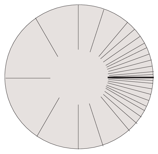
Refer to caption — Figure 1. An example of a domain whose boundary has a non-trivial prime end. Note that if an impression of a fundamental chain contains the point $1\in\partial W$ , then it contains the whole segment $S_{0}$ .

We define the Carathéodory compactification $\widehat{W}$ to be the disjoint union of $W$ and the set of prime ends of $W$ with the following topology. For any crosscut neighborhood $N$ let $\widetilde{N}\subset\widehat{W}$ be the neighborhood $N$ itself, and the collection of all prime ends which can be represented by fundamental chains starting with $N$ . These neighborhoods, together with the open subsets of $W$ , form the basis for the topology of $\widehat{W}$ .

Carathéodory Theorem.

Every conformal isomorphism $\phi:W\to{\mathbb{D}}$ extends uniquely to a homeomorphism

\hat{\phi}:\widehat{W}\to\overline{{\mathbb{D}}}.

Carathéodory Theorem for locally connected domains is a synthesis of the above statement and Proposition 3.1.

Let us note:

Lemma 3.2.

If $f$ is a continuous map from a compact locally connected space $X$ onto a Hausdorff space $Y$ , then $Y$ is also locally connected.

Proof.

We reproduce the proof from [18], p. 184. The image $f(X)=Y$ is compact. For any point $y\in Y$ and any open neighborhood $N=N(y)\subset Y$ the set $f^{-1}(N)$ is an open neighborhood of the compact set $f^{-1}(y)\subset X$ . Consider the family $V_{\alpha}$ of all connected subsets of $f^{-1}(N)$ , which intersect $f^{-1}(y)$ . Then the union $\cup f(V_{\alpha})$ is a connected subset of $N$ . It is also a neighborhood of $y$ , since it contains the open neighborhood $Y\setminus f(X\setminus\cup V_{\alpha})$ of $y$ . ∎

So, in particular, a Jordan curve is a locally connected set. Using Carathéodory Theorem and Lemma 3.2, we see that the converse to Proposition 3.1 also holds:

Proposition 3.3.

If the impression of every prime end of $W$ is trivial then $\partial W$ is locally connected.

We also note:

Theorem 3.4.

In the case when $W$ is Jordan, the identity map $W\to W$ extends to a homeomorphism between the Carathéodory closure $\widehat{W}$ and $\overline{W}$ .

Proof.

Suppose that there is a point $x\in\partial W$ which is in the impression of two different prime ends $p_{1}$ , $p_{2}$ . Let $N_{1}$ , $N_{2}$ be two disjoint crosscut neighborhoods of $p_{1}$ , $p_{2}$ respectively in $\hat{W}$ . By Carathéodory Theorem, there exist continuous paths

\gamma_{i}:[0,1)\to\overset{\circ}{N}_{i}\text{ such that }\lim_{t\to 1-}\gamma_{i}(t)=x.

Let $\gamma$ be a simple curve in $W$ which is disjoint from $\gamma_{i}((0,1))$ and connects $\gamma_{1}(0)$ to $\gamma_{2}(0)$ . Then

\Gamma\equiv\gamma_{1}([0,1))\cup\gamma_{2}([0,1))\cup\gamma\cup\{x\}

is a Jordan curve which is easily seen to disconnect $\partial W$ . Since

\Gamma\cap\partial W=\{x\},

removing a single point $x$ disconnects $\partial W$ . Hence $\partial W$ is not a Jordan curve, which contradicts our assumptions.

We define a map $\iota:\widehat{W}\to\overline{W}$ by

•

$\iota(x)=x$ for $x\in W$ ;
•

$\iota(p)={\cal I}(p)$ for a prime end $p$ .

Continuity and surjectivity of $\iota$ are evident from its definition. Its injectivity was shown above. Since a continuous bijection of a compact set to a Hausdorff topological space is a homeomorphism onto the image, the proof is completed. ∎

In the Jordan case, we will use the notation $\overline{\phi}$ for the extension of a conformal map to the closure of $W$ . Of course,

\overline{\phi}=(\overline{f})^{-1}.

Carathéodory compactification of $(W,w)$ can be seen as its metric completion for the following metric. Let $z_{1}$ , $z_{2}$ be two points in $W$ distinct from $w$ . We will define the crosscut distance $\operatorname{dist}^{W}_{C}(z_{1},z_{2})$ between $z_{1}$ and $z_{2}$ as the infimum of the diameters of curves $\gamma$ in $W$ with the following properties:

•

$\gamma$ is either a crosscut or a simple closed curve;
•

$\gamma$ separates $z_{1}$ , $z_{2}$ from $w$ .

It is easy to verify that:

Theorem 3.5.

The crosscut distance is a metric on $W\setminus\{w\}$ which is locally equal to the Euclidean one. The completion of $W$ equipped with $\operatorname{dist}_{C}$ is homeomorphic to $\widehat{W}$ .

3.2. Computational representation of prime ends

Definition 3.1.

We say that a curve $g:(0,1)\to{\mathbb{C}}$ is a rational polygonal curve if:

•

the image of $g$ is a simple curve;
•

$g$ is piecewise-linear with rational coefficients.

The following is elementary:

Proposition 3.6.

Let $N_{\gamma_{j}}$ be a fundamental chain in a pointed simply-connected domain $(W,w)$ . Then there exists an equivalent fundamental chain $N_{\tau_{j}}$ such that the following holds. For every $j$ there exists a rational polygonal curve $t_{j}:(0,1)\to{\mathbb{C}}$ with

t_{j}(0.5)\in N_{\gamma_{j}}\setminus\overline{N_{\gamma_{j+1}}},

and such that $\tau_{j}\subset t_{j}([0.1,0.99])$ . Furthermore, $t_{j}$ can be chosen so that

\operatorname{diam}t_{j}(0,1)\underset{j\to\infty}{\longrightarrow}0.

We call the sequence of polygonal curves $t_{j}$ as described in the above proposition a representation of the prime end $p$ specified by $N_{\gamma_{j}}$ . Since only a finite amount of information suffices to describe each rational polygonal curve $t_{j}$ , the sequence $t_{j}$ can be specified by an oracle. Namely, there exists an algorithm ${\cal A}$ such that for every representation $(t_{j})$ of a prime end there exists a function $\phi:{\mathbb{N}}\to{\mathbb{N}}$ such that given access to the values of $\phi(i),$ $i=1,\ldots,n$ , the algorithm ${\cal A}$ outputs the coefficients of the rational polygonal curves $t_{j}$ , $j=1,\ldots,m_{n}$ with $m_{n}\underset{n\to\infty}{\longrightarrow}\infty$ . We will refer to such $\phi$ simply as an oracle for $p$ .

3.3. Structure of a computable metric space on $\widehat{W}$ .

Let $K\Subset{\mathbb{C}}$ . We say that $\phi$ is an oracle for $K$ if $\phi$ is a function from the natural numbers to sets of finite sequences of triples $(x_{j},y_{j},r_{j})$ of rational numbers with the following property. Let

\phi(n)=\{(x_{j},y_{j},r_{j})\}_{j=1}^{k_{n}},

and let $B_{j}$ be the ball of radius $r_{j}$ about the point $x_{j}+iy_{j}$ . Then

\operatorname{dist}_{H}(\bigcup_{j=1}^{k_{n}}\overline{B_{j}},K)<2^{-n}.

Let $(W,w)$ be a simply-connected pointed domain. Then the following conditional computability result holds:

Theorem 3.7.

The following is true in the presence of oracles for $w$ and for $\partial W$ . The Carathéodory completion $\widehat{W}$ equipped with the crosscut distance is a computable metric space, whose ideal points are rational points in $W$ . Moreover, this space is computably compact.

Proof.

First observe that from $w$ and $\partial W$ , one can lower compute the open sets $W$ and ${\mathbb{C}}\setminus\overline{W}$ . In particular, we can for example enumerate all the ideal points in $\text{Comp}({\mathbb{C}})$ which are contained in $W$ . Similarly, one can enumerate all the ideal points in $\text{Comp}({\mathbb{C}})$ which are disjoint from $\overline{W}$ . With this in mind, let us describe the algorithm ${\cal A}$ which uniformly computes the crosscut distance between two ideal points $s_{1}$ , $s_{2}$ with precision $2^{-k}$ :

(1)

$n:=1$ ;
(2)

compute a closed domain $L_{n}\subset W$ which is an ideal point in $\text{Comp}({\mathbb{C}})$ such that $\operatorname{dist}_{H}(L_{n},\overline{W})<2^{-n}$ (in order to do this, query the oracle to obtain $S_{n}\supset\partial W$ which is a $2^{-(n+1)}$ -approximation of the boundary $\partial W$ , and let $L_{n}$ be the closure of the union of bounded connected components of the complement ${\mathbb{C}}\setminus S_{n}$ );
(3)

compute a closed domain $U_{n}\supset W$ which is an ideal point in $\text{Comp}({\mathbb{C}})$ such that $\operatorname{dist}_{H}(U_{n},\overline{W})<2^{-n}$ (this is done similarly to the previous step);
(4)

if $s_{1}$ and $s_{2}$ do not lie in $L_{n}$ , then go to step (8), else continue;
(5)

compute a lower bound $l_{n}$ on $\operatorname{dist}_{C}^{U_{n}}(s_{1},s_{2})$ such that $|l_{n}-\operatorname{dist}_{C}^{U_{n}}(s_{1},s_{2})|<2^{-n}$ ;
(6)

compute an upper bound $u_{n}$ on $\operatorname{dist}_{C}^{L_{n}}(s_{1},s_{2})$ such that $|u_{n}-\operatorname{dist}_{C}^{L_{n}}(s_{1},s_{2})|<2^{-n}$ ;
(7)

if $|l_{n}-u_{n}|<2^{-k}$ output $l_{n}$ and exit;
(8)

$n:=n+1$ ;
(9)

go to (2)

The correctness of the argument follows from elementary continuity considerations.

The proof of computable compactness of $\widehat{W}$ is similarly straightforward, and is left to the reader.

∎

3.4. Moduli of locally connected domains

Suppose $\partial W$ is locally connected. The following definition is standard:

Definition 3.2 (Modulus of local connectivity).

Let $X\subset{\mathbb{R}}^{2}$ is a connected set. Any strictly increasing function $m:(0,a)\to{\mathbb{R}}$ is called a modulus of local connectivity of $X$ if

•

for all $x,y\in X$ such that $\operatorname{dist}(x,y)<r<a$ there exists a connected subset $L\subset X$ containing both $x$ and $y$ with the property $\operatorname{diam}(L)<m(r)$ ;
•

$m(r)\searrow 0$ as $r\searrow 0$ .

Of course, the existence of a modulus of local connectivity implies that $X$ is locally connected. Conversely, every compact connected and locally connected set has a modulus of local connectivity.

We note that every modulus of local connectivity is also a modulus of path connectivity:

Proposition 3.8.

Let $m(r)$ be a modulus of local connectivity for a connected set $X\subset{\mathbb{R}}^{2}$ . Let $x,y\in X$ such that $\operatorname{dist}(x,y)<r$ . Then there exists a path $\ell$ between $x$ and $y$ with diameter at most $m(r)$ .

For the proof, see Proposition 2.2 of [6].

Definition 3.3 (Carathéodory modulus).

Let $(W,w)$ be a pointed simply-connected domain. A strictly increasing function $\eta:(0,a)\to{\mathbb{R}}$ is called the Carathéodory modulus if for every crosscut $\gamma$ with $\operatorname{diam}(\gamma)<r<a$ we have $\operatorname{diam}N_{\gamma}<\eta(r)$ .

We note:

Proposition 3.9.

There exists a Carathéodory modulus $\eta(r)$ such that $\eta(r)\searrow 0$ when $r\searrow 0$ if and only if the boundary $\partial W$ is locally connected.

Proof.

Let us begin by assuming that there exists a Carathéodory modulus with $\eta(r)\searrow 0$ . Then the impression of every prime end of $(W,w)$ is a single point. By Carathéodory Theorem, this implies that $\partial W$ is a continuous image of the circle, and hence, is locally connected.

Arguing in the other direction, if $\partial W$ is locally connected, then by Proposition 3.1 every fundamental chain shrinks to a single boundary point. The existence of a desired Carathéodory modulus follows from compactness considerations.

∎

4. Statements of the main results

To simplify the exposition, we present our results for bounded domains only. However, all the theorems we formulate below may be stated for general simply-connected domains on the Riemann sphere ${\widehat{{\mathbb{C}}}}$ . In this case, the spherical metric on ${\widehat{{\mathbb{C}}}}$ would have to be used instead of the Euclidean both in the statements and in the proofs.

Our first result is the following:

Theorem 4.1.

Suppose $(W,w)$ is a bounded simply-connected pointed domain. Suppose the Riemann mapping

\phi:W\to{\mathbb{D}}\text{ with }\phi(w)=0,\;\phi^{\prime}(w)>0

is computable. Then there exists an algorithm ${\cal A}$ which, given a representation of a prime end $p\in\widehat{W}$ computes the value of $\hat{\phi}(p)\in S^{1}.$

In view of Theorem 2.10, we have:

Corollary 4.2.

Suppose we are given oracles for $W$ as a lower-computable open set, and for $\partial W$ as a lower-computable closed set, and an oracle for the value of $w$ as well. Given a representation of a prime end $p\in\widehat{W}$ , the value $\hat{\phi}(p)\in S^{1}$ is uniformly computable.

To state a “global” version of the above computability result, we use the structure of a computable metric space:

Theorem 4.3.

In the presence of oracles for $w$ and for $\partial W$ , both the Carathéodory extension

\hat{\phi}:\widehat{W}\to\overline{{\mathbb{D}}}\text{ and its inverse }\hat{f}\equiv\hat{\phi}^{-1}:\overline{{\mathbb{D}}}\to\widehat{W}

are computable, as functions between computable metric spaces.

Remark 4.1.

Note that the assumptions of Theorem 4.3 are stronger than those of Corollary 4.2: computability of $\partial W$ implies lower computability of $W$ and $\partial W$ , but not vice versa.

Proof.

The assertion that computability of $\partial W$ implies lower computability of $W$ and $\partial W$ is straightforward from the definitions.

To show that the converse statement does not hold consider the following example. Let $B\subset{\mathbb{N}}$ be a lower-computable, non-computable set, and let ${\cal A}$ be an algorithm which enumerates the elements of $B$ . Let $I$ be the boundary of the unit square $I\equiv\partial([0,1]\times[0,1])$ . Set $x_{i}=1-1/{2i}$ . We now modify $I$ about the points $x_{i}$ . If $i\notin B$ , we do nothing. If $i\in B$ and it is enumerated by ${\cal A}$ at step $s$ , then remove the segment from $(x_{i}-s_{i},1)$ to $(x_{i}+s_{i},1)$ where

s_{i}=\min\{2^{-s},1/(3i^{2})\},

and add straight segments connecting $(x_{i}-s_{i},1)$ to $(x_{i}-s_{i},1.5)$ to $(x_{i}+s_{i},1.5)$ to $(x_{i}+s_{i},1)$ (we call such a decoration an $i$ -peninsula of width $s_{i}$ ). Denote $S$ thus obtained set and let $W$ be the bounded connected component of ${\mathbb{C}}\setminus S$ .

Note that computability of $\partial W=S$ would imply computability of $B$ : to check whether $i\in B$ it is sufficient to see whether $S$ has an $i$ -peninsula, which is equivalent to $(x_{i},1.5)\in S$ . Hence, $\partial W$ is not computable.

However, $\partial W$ is lower computable. Indeed, to lower compute $\partial W$ , start by drawing $I$ with the segments $(x_{i}-1/(3i^{2}),x_{i}+1/(3i^{2}))$ removed. Then emulate the algorithm ${\cal A}$ enumerating $B$ and at each step $s$ :

•

if $i$ is enumerated, then draw the corresponding $i$ -fjord about $x_{i}$ .
•

For every $j<s$ that has not been enumerated so far, narrow the removed segment $(x_{j}-1/(3i^{2}),x_{j}+1/(3i^{2}))$ to $(x_{j}-s_{i},x_{j}+s_{i})$ .

Similarly, the domain $W$ is lower computable. The procedure to lower compute it is the following: start by drawing the unit square $[0,1]\times[0,1]$ . Then emulate the algorithm ${\cal A}$ enumerating $B$ and at each step $s$ :

•

if $i$ is enumerated, add the rectangle bounded by straight segments from $(x_{i}-s_{i},1)$ to to $(x_{i}-s_{i},1.5)$ to $(x_{i}+s_{i},1.5)$ to $(x_{i}+s_{i},1)$ to $(x_{i}-s_{i},1)$ .

∎

For a domain $W$ with a locally connected boundary, we may ask when the map $\overline{f}:\overline{{\mathbb{D}}}\to\overline{W}$ is computable. We are able to give a sharp result:

Theorem 4.4.

Suppose $(W,w)$ is a pointed simply-connected bounded domain with a locally connected boundary. Assume that the Riemann map

f:{\mathbb{D}}\to W\text{ with }f(0)=w,\;f^{\prime}(0)>0

is computable.

Then the boundary extension

\overline{f}:\overline{{\mathbb{D}}}\to\overline{W}

is computable if and only if there exists a computable Carathéodory modulus $\eta(r)$ with $\eta(r)\searrow 0$ as $r\searrow 0$ .

Remark 4.5.

With routine modifications, the above result can be made uniform in the sense that there is an algorithm which from a description of $f$ and $\eta$ computes a description of $\overline{f}$ , and there is an algorithm which from a description of $\overline{f}$ computes a Carathéodory modulus $\eta$ . See for example [9] for statements made in this generality.

We note that the seemingly more “exotic” Carathéodory modulus cannot be replaced by the modulus of local connectivity in the above statement:

Theorem 4.6 (Computational Incommensurability of Moduli ).

There exists a simply-connected domain $W$ such that $\partial W$ is locally-connected, $\overline{W}$ is computable, and there exists a computable Carathéodory modulus $\eta(r)$ , however, no computable modulus of local connectivity exists for $\partial W$ .

Finally, we turn to computational complexity questions in the cases when $\hat{\phi}$ or $\overline{f}$ are computable. We show that:

Theorem 4.7.

Let $q:{\mathbb{N}}\to{\mathbb{N}}$ be any computable function. There exist Jordan domains $W_{1}\ni 0$ , $W_{2}\ni 0$ such that the following holds:

•

the closures $\overline{W}_{1}$ , $\overline{W}_{2}$ are computable;
•

the extensions $\overline{\phi}:\overline{W}_{1}\to\overline{{\mathbb{D}}}$ and $\overline{f}:\overline{{\mathbb{D}}}\to\overline{W}_{2}$ are both computable functions;
•

the time complexity of $\overline{f}$ and $\overline{\phi}$ is bounded from below by $q(n)$ for large enough values of $n$ .

5. Preliminaries from Complex Analysis

5.1. Distortion Theorems

We will make use of two standard results in Complex Analysis.

Koebe One-Quarter Theorem.

Let $f:{\mathbb{D}}\to W$ be a conformal isomorphsim, and let $w=f(0)$ . Then the distance from $w$ to the boundary of $U$ is at least $\frac{1}{4}|f^{\prime}(0)|$ .

Koebe Distortion Theorem.

Let $f:{\mathbb{D}}\to{\mathbb{D}}$ be a conformal mapping with the properties $f(0)=0$ and $f^{\prime}(0)=1$ . Then for every $z\in{\mathbb{D}}$ ,

\frac{1-|z|}{(1+|z|^{3})}\leq|f^{\prime}(z)|\leq\frac{1+|z|}{(1-|z|^{3})}.

5.2. Harmonic Measure

A detailed discussion of harmonic measure can be found in [8]. Here we briefly recall some of the relevant facts. We will only define harmonic measure for a finitely-connected domain $W\subset\widehat{\mathbb{C}}$ . Recall that a connected subdomain of ${\widehat{{\mathbb{C}}}}$ is called hyperbolic if its complement contains at least three points. We start with the following well-known fact:

Proposition 5.1.

Let $W$ be a finitely-connected hyperbolic subdomain of $\widehat{\mathbb{C}}$ , and $w\in W$ . Then the Brownian path originating at $w$ hits the boundary of $W$ with probability $1$ .

Let $W$ be a finitely-connected hyperbolic domain in ${\widehat{{\mathbb{C}}}}$ , and $w\in W$ . The harmonic measure $\omega_{W,w}$ is defined on the boundary $\partial W$ . For a set $E\subset\partial W$ it is equal to the probability that the Brownian path originating at $w$ will first hit $\partial W$ within the set $E$ .

By way of an example, consider a simply-connected hyperbolic domain $W\subset{\widehat{{\mathbb{C}}}}$ with locally-connected boundary, let $w$ be an arbitrary point of $W$ . Consider the unique conformal Riemann mapping

\psi:W\to{\mathbb{D}},\text{ with }\psi(w)=0\text{ and }\psi^{\prime}(w)>0.

By Carathéodory Theorem, $\psi^{-1}$ extends continuously to map $\overline{W}\to\bar{\mathbb{D}}$ . By symmetry considerations, the harmonic measure $\omega_{{\mathbb{D}},0}$ coincides with the Lebesgue measure $\mu$ on the unit circle $S^{1}=\partial{\mathbb{D}}$ . Conformal invariance of Brownian motion implies that $\omega_{W,w}$ is obtained by pushing forward $\mu$ by $\psi^{-1}|_{S^{1}}$ .

We will repeatedly use the following estimate on the harmonic measure

Proposition 5.2 (Majoration principle).

Let $W^{\prime}\subset W$ be two finitely-connected hyperbolic domains in ${\widehat{{\mathbb{C}}}}$ . Let $w\in W^{\prime}$ . Let

K_{1}=\partial W\cap\partial W^{\prime},\;K_{2}=\partial W\setminus K_{1},\;K_{3}=\partial W^{\prime}\setminus K_{1}.

Then

\omega_{W,w}(K_{2})\leq\omega_{W^{\prime},w}(K_{3}).

Proof.

Evidently, the Brownian path originating at $w$ which exits $W$ through $K_{2}$ must exit $W^{\prime}$ through $K_{3}$ . The statement now follows from the definition of harmonic measure. ∎

The proof of the following classical result can be found in [8]:

Beurling Projection Theorem.

If $K\subset\bar{\mathbb{D}}\setminus\{0\}$ , and $K^{*}\equiv\{|w|\;:\;w\in K\}$ is the circular projection of $K$ , then for every $z\in{\mathbb{D}}\setminus K$

\omega_{{\mathbb{D}}\setminus K,z}(K)\geq\omega_{{\mathbb{D}}\setminus K^{*},-|z|}(K^{*}).

5.3. Estimating the variation of $f:{\mathbb{D}}\to W$ (Warshawski’s Theorems).

We will quote several results from the beatifully concise paper of S.E. Warshawski [23]. Let us consider a conformal map $f:{\mathbb{D}}\to W$ . Without assuming that $W$ is necessarily Jordan, we can make the following definition.

Definition 5.1.

Let $|z_{0}|=1.$ For $0<r<1$ , define

{\cal O}(r;z_{0})=\underset{|z_{k}-z_{0}|\leq r}{\sup}|f(z_{1})-f(z_{2})|\text{ where }|z_{1}|<1,\;|z_{2}|<1,

and

{\cal O}(r)=\underset{|z_{0}|=1}{\sup}{\cal O}(r;z_{0}).

The quantity ${\cal O}(r)$ is called the oscillation of $f(z)$ at the boundary.

The first theorem in [23] is the following:

Theorem 5.3.

Suppose $W\ni 0$ is a simply-connected bounded region, and $f:{\mathbb{D}}\to W$ is a conformal mapping such that $f(0)=0$ . Assume that $\eta(r)$ is a Carathéodory modulus of $(W,0)$ . If $A$ denotes the area of $W$ , then the oscillation of $f(z)$ at the boundary

{\cal O}(r)\leq\eta\left(\left(\frac{2\pi A}{\log 1/r}\right)^{1/2}\right),\text{ for all }r\in(0,1).

The proof follows easily from Wolff’s Lemma [25]:

Lemma 5.4.

Suppose that $f$ is a conformal mapping of ${\mathbb{D}}$ onto a simply-connected bounded region $W$ . Let $z_{0}\in S^{1}$ , and let $k_{r}$ be the arc of the circle $|z-z_{0}|=r$ which is contained in ${\mathbb{D}}$ . Then for every $r\in(0,1)$ there exists $\rho^{*}\in(r,\sqrt{r})$ such that the image of $k_{\rho^{*}}$ is a crosscut of $W$ of length

\ell_{\rho^{*}}\leq\left(\frac{2\pi A}{\log 1/r}\right)^{1/2}.

(5.1)

Proof.

We introduce polar coordinates about $z_{0}$ and write, for $\rho\in(0,1),$

\ell_{\rho}=\int_{k_{\rho}}|f^{\prime}(z)||dz|=\int_{k_{\rho}}|f^{\prime}(z_{0}+\rho e^{i\theta})|\rho d\theta\leq+\infty.

By Cauchy-Schwarz-Buniakowsky Inequality,

\ell_{\rho}^{2}\leq\int_{k_{\rho}}|f^{\prime}(z_{0}+\rho e^{i\theta})|^{2}\rho d\theta\int_{k_{\rho}}\rho d\theta\leq\pi\rho\int_{k_{\rho}}|f^{\prime}(z+\rho e^{i}\theta)|^{2}\rho d\theta.

Integrating with respect to $\rho$ from $r$ to $\sqrt{r}$ , we obtain

\int_{r}^{\sqrt{r}}\frac{\ell_{\rho}^{2}}{\rho}d\rho<\int_{0}^{\sqrt{r}}\frac{\ell_{\rho}^{2}}{\rho}d\rho\leq\pi\int_{0}^{\sqrt{r}}\int_{k_{\rho}}|f^{\prime}(z_{0}+\rho e^{i\theta})|^{2}\rho d\theta<\pi A.

Hence, there exists $\rho^{*}\in(r,\sqrt{r}),$ such that

\ell_{\rho^{*}}^{2}\int_{r}^{\sqrt{r}}\frac{d\rho}{\rho}=\frac{1}{2}\ell_{\rho^{*}}^{2}\log\frac{1}{r}<\pi A.

Since the image of $k_{\rho^{*}}$ has a finite length, it is a crosscut in $W$ , and the proof is completed.

∎

Proof of Theorem 5.3.

Let

T_{r}\equiv f(\{|z-z_{0}|<r,\;|z|<1\})\subset W.

Select $\rho^{*}\in(r,\sqrt{r})$ so that (5.1) holds. Then $T_{r}\subset T_{\rho^{*}}$ . The image

\gamma\equiv f(k_{\rho^{*}})

is a crosscut of $W$ with $\operatorname{diam}\gamma\leq\ell_{\rho^{*}}.$ Hence, by definition of a Carathéodory modulus,

\operatorname{diam}T_{r}\leq\operatorname{diam}T_{\rho^{*}}\leq\eta\left(\left(\frac{2\pi A}{\log 1/r}\right)^{1/2}\right).

If $z_{1},z_{2}\in{\mathbb{D}}\cap\{|z-z_{0}|<r\},$ then $f(z_{1})$ , $f(z_{2})\in T_{r}$ , and the proof is completed. ∎

We quote another theorem of [23] without a proof. First, we make a definition:

Definition 5.2.

Let $W_{1}$ and $W_{2}$ be two simply-connected regions. Let us define the inner distance between $W_{1}$ , $W_{2}$ as

\operatorname{dist}_{i}(W_{1},W_{2})\equiv\max(d(\partial W_{1}\cap\overline{W}_{2},\partial W_{2}),d(\partial W_{2}\cap\overline{W}_{1},\partial W_{1}),

where, as usual, $d(X,Y)$ denotes the “one-sided” distance

d(X,Y)=\sup_{x\in X}\inf_{y\in Y}\operatorname{dist}(x,y).

Theorem 5.5.

Suppose $W_{i}\ni 0$ for $i=1,2$ are two simply-connected bounded regions. Let $\sigma=\operatorname{dist}(0,\partial W_{1}\cup\partial W_{2}).$ Suppose $\operatorname{dist}_{i}(W_{1},W_{2})<\epsilon$ where $\epsilon\in(0,1)$ and $\epsilon<\sigma/64.$ Let $\eta_{i}(r)$ denote the Carathéodory modulus of $W_{i}$ . Let $A_{i}$ be the area of $W_{i}$ . Denote $f_{i}(z)$ the conformal map ${\mathbb{D}}\to W_{i}$ with $f_{i}(0)=0$ , $f_{i}^{\prime}(0)>0$ . Then for $z\in{\mathbb{D}}$ we have

|f_{1}(z)-f_{2}(z)|\leq\left(1+\frac{k}{\sigma^{1/2}}\epsilon^{1/4}\log\frac{4}{\epsilon}\right)\left[\eta_{1}\left(\left(\frac{8\pi A_{1}}{\log(1/\epsilon)}\right)^{1/2}\right)+\eta_{2}\left(\left(\frac{8\pi A_{2}}{\log(1/\epsilon)}\right)^{1/2}\right)\right],

where $k$ is a constant $k\leq 16e$ .

6. Proofs

6.1. Proof of Theorem 4.1

We will show that from a computable description $\{\gamma_{i}\}$ of a prime end $p$ , we can compute a description of the point $z=\hat{\varphi}(p)\in\partial{D}$ . We will describe an algorithm that, given $\{A_{i}\}$ and $\epsilon$ , will find $z^{\prime}\in D$ such that $|z-z^{\prime}|\leq\epsilon$ . The following proposition will give us the key estimate.

Proposition 6.1.

Let $W$ be a connected domain with $\infty\not\in W$ . Let $\gamma$ be a crosscut of $W$ , $\operatorname{dist}(\gamma,w)\geq M$ , for some $M>0$ and $N_{\gamma}$ be the component of $W\setminus\gamma$ not containing $w$ . Assume that $\epsilon^{2}<M/4$ . Then

\operatorname{diam}(\gamma)\leq\epsilon^{2}\implies\operatorname{diam}(\varphi(N_{\gamma}))\leq\frac{30\epsilon}{\sqrt{M}}.

Similar statements are well-known in the literature, likely beginning with the works of Lavrientieff [13] and Ferrand [7]. As an immediate corollary, we obtain

Corollary 6.2.

Let $h(\delta)$ be a modulus of fluctuation of $f=\varphi^{-1}$ . Then we have the following estimate for Caratheodory modulus:

\eta(\epsilon^{2})\leq h\left(\frac{30\epsilon}{\sqrt{M}}\right).

Proof.

Let two points $w_{1}$ and $w_{2}$ be separated from $w$ by a crosscut of length at most $\epsilon^{2}$ . Let $z_{1,2}=\phi(w_{1,2})$ . By Proposition 6.1, $|z_{1}-z_{2}|\leq\frac{30\epsilon}{\sqrt{M}}$ . Thus

|w_{1}-w_{2}|=|f(z_{1})-f(z_{2})|\leq\frac{30\epsilon}{\sqrt{M}}.

∎

Let us now to turn to the proof of Proposition 6.1. We use the following lemmas.

Lemma 6.3.

If $\operatorname{diam}(\gamma)<\epsilon^{2}$ then for any $z\in\varphi(\gamma)$ ,

|z|>1-\frac{3\epsilon}{\sqrt{M}}.

Proof.

Let $f=\varphi^{-1}$ and let $w=f(0)\in W$ . By Koebe One-Quarter Theorem, $|f^{\prime}(0)|\geq 4M$ . By Koebe Distortion Theorem,

|f^{\prime}(z)|\geq 4M\frac{1-|z|}{(1+|z|)^{3}}\geq M\frac{1-|z|}{2}.

Another application of Koebe One-Quarter Theorem gives

\operatorname{dist}(f(z),\partial W)\geq\frac{1}{4}(1-|z|)|f^{\prime}(z)|\geq M\frac{(1-|z|)^{2}}{8}.

Notice now that since $\gamma$ is a crosscut,

\operatorname{diam}(\gamma)\geq\operatorname{dist}(f(z),\partial W)\geq M\frac{(1-|z|)^{2}}{8}.

The lemma immediately follows from the last inequality.

∎

Lemma 6.4.

Let $\gamma$ be a crosscut of $W$ and let $M=\operatorname{dist}(\gamma,w)$ . Let

\operatorname{diam}(\gamma)\leq\epsilon^{2}<M/4.

Suppose $\varphi(\gamma)\subset\bar{D}$ ends at $z_{1}$ and $z_{2}$ , then

|z_{1}-z_{2}|<\frac{8\epsilon}{\sqrt{M}}.

In addition, if $K$ is the part of $\partial W$ separated by $\gamma$ from $w$ , then

\omega_{W,w}(K)\leq\frac{4\epsilon}{\pi\sqrt{M}}.

Proof.

First observe that by conformal invariance of harmonic measure

\text{length of arc}[z_{1},z_{2}]=2\pi\omega_{W,w}(K).

Thus

|z_{1}-z_{2}|\leq 2\pi\omega_{W,w}(K),

so the second statement of the Lemma implies the first one.

Let $x$ be any point of $\gamma$ , and let $W^{\prime}$ be the component of $W\setminus B(x,\epsilon^{2})$ containing $w$ . Let $K_{1}=\partial W^{\prime}\cap\partial B(x,\epsilon^{2})$ and $K_{2}=\partial W^{\prime}\setminus K_{1}$ . Since $\operatorname{diam}\gamma\leq\epsilon^{2}$ , we see that $W^{\prime}$ is simply-connected. Thus we can apply the Majoration Principle (Proposition 5.2) to show that

\omega_{W,w}(K)\leq\omega_{W^{\prime},w}(K_{1}).

(6.1)

We will use Beurling Projection Theorem to obtain an upper bound on $\omega_{W^{\prime},w}(K_{1})$ . By applying a shift by $-x$ and a rotation, we may assume that $x=0$ and that $w$ lies on the negative real axis.

Let us consider the inversion map $g(w)=\frac{\epsilon^{2}}{w}$ . It maps $W^{\prime}$ to a subdomain $g(W^{\prime})\subset{\mathbb{D}}$ . We set

w^{\prime}=g(w),\;K^{\prime}_{1}=g(K_{1})=\partial g(W^{\prime})\cap S^{1},\;K^{\prime}_{2}=g(K_{2})=\partial g(W^{\prime})\cap{\mathbb{D}}.

Let $K^{*}_{2}$ be the circular projection of $K_{2}^{\prime}$ . Since by our assumptions $w^{\prime}=-|w^{\prime}|$ , Beurling Projection Theorem implies that

\omega_{g(W^{\prime}),w^{\prime}}(K^{\prime}_{2})\geq\omega_{{\mathbb{D}}\setminus K^{*}_{2},w^{\prime}}(K^{*}_{2}),

or, since $\omega_{g(W^{\prime}),w^{\prime}}(K^{\prime}_{2})+\omega_{g(W^{\prime}),w^{\prime}}(K^{\prime}_{1})=1$ and $\omega_{{\mathbb{D}}\setminus K^{*}_{2},w^{\prime}}(K^{*}_{2})+\omega_{{\mathbb{D}}\setminus K^{*}_{2},w^{\prime}}(S^{1})=1$ ,

\omega_{g(W^{\prime}),w^{\prime}}(K^{\prime}_{1})\leq\omega_{{\mathbb{D}}\setminus K^{*}_{2},w^{\prime}}(S^{1})

Now we can use the conformal invariance of harmonic measure to see that

\omega_{W^{\prime},w}(K_{1})\leq\omega_{g^{-1}\left({\mathbb{D}}\setminus K^{*}_{2}\right),w}(\partial B(x,\epsilon^{2}))

Another application of the Majoration Principle (Proposition 5.2) shows that

\omega_{W^{\prime},w}(K_{1})\leq\omega_{w,W_{0}}(\partial B(x,\epsilon^{2})),

where $W_{0}={\widehat{{\mathbb{C}}}}\setminus(B(x,\epsilon^{2})\cup[0,\infty))$ .

The last quantity can be shown to be equal to

\frac{4}{\pi}\tan^{-1}\left(\frac{\epsilon}{\sqrt{M}}\right)\leq\frac{4\epsilon}{\pi\sqrt{M}}

(see [8], page 107). The estimate together with inequality (6.1) immediately implies the second statement of the lemma. ∎

Proof of the Proposition 6.1.

We first show that the radial projection of $\varphi(\gamma)$ onto the unit circle has the length bounded by $\frac{25\epsilon}{\sqrt{M}}$ . Let this projection be the arc $[z^{\prime}_{1},z^{\prime}_{2}]$ .

Let us first estimate $|z^{\prime}_{1}-z_{1}|$ . Without loss of generality we can assume that $z^{\prime}_{1}=1$ . Let

r=\max\left\{x>0\ :\ x\in\varphi(\gamma)\right\},\;w=\varphi^{-1}(r)=f(r)\text{ and }I=[r,1].

Let $\gamma^{\prime}$ be the arc of $\gamma$ joining $w$ to the end of $\gamma$ corresponding to $z_{1}$ . Then $\gamma^{\prime}$ is a crosscut of the domain $W^{\prime}=W\setminus f(I)$ with

\operatorname{dist}(w,\partial W^{\prime})\geq M-\epsilon^{2}\geq M/2.

Let $K^{\prime}$ be the part of the boundary of $W^{\prime}$ separated by $\gamma^{\prime}$ from $w$ . By Lemma 6.4,

\omega_{W^{\prime},w}(K^{\prime})\leq\frac{4\sqrt{2}\epsilon}{\pi\sqrt{M}}.

Notice now that by invariance of harmonic measure and symmetry we have

\omega_{W^{\prime},w}(K^{\prime})=\omega_{{\mathbb{D}}\setminus I,0}(\phi(K))=\frac{1}{2}\omega_{{\mathbb{D}}\setminus I,0}(I\cup[z_{1},\overline{z_{1}}]),

where $[z_{1},\overline{z_{1}}]$ denote here the arc of the unit circle joining $z_{1}$ and $\overline{z_{1}}$ .

Another application of majoration principle shows that

|z_{1}-z^{\prime}_{1}|\leq 1/2\text{ length of }[z_{1},\overline{z_{1}}]=\pi\omega_{{\mathbb{D}},0}(I\cup[z_{1},\overline{z_{1}}])\leq\pi\omega_{{\mathbb{D}}\setminus I,0}(I\cup[z_{1},\overline{z_{1}}])\leq\frac{12\epsilon}{\sqrt{M}}.

Since the same estimate holds for $|z_{1}-z^{\prime}_{2}|$ , we get the desired estimate on the length of the projection.

To obtain the statement of the proposition, we just need to combine this estimate with Lemma 6.3.

∎

We are now ready to prove Theorem 4.1.

Proof of Theorem 4.1.

Consider a computable representation $(t_{j})$ of the crosscut $p$ . To compute $\phi(p)$ with presicion $\delta$ , we compute $j$ such that $\operatorname{diam}t_{j}<10^{-3}M\delta^{2}$ , where $M$ is a lower estimate on the distance from $t_{1}$ to $w$ . Then we compute $\phi(t_{j}(1/2))$ with presicion $10^{-3}\delta$ . By Proposition 6.1, this value is within $\delta$ of $\phi(p)$ . ∎

6.2. Proof of Theorem 4.3

Let us show that $\hat{\phi}$ is computable, computability of $\hat{f}$ will follow from Theorem 2.12.

Note that given oracles for $\partial\Omega$ and $w$ , the Caratheodory distance between two interior points is computable by using, say, computable interior polinomial approximation.

Let now $x_{n}\to x$ be a sequence of ideal points in $\widehat{W}$ with $\operatorname{dist}_{C}^{W}(x_{n},x)<2^{-n}$ . We compute a rational number $M>0$ , which is a lower bound on $\operatorname{dist}(x,w)$ . We set

\epsilon_{k}=\frac{\sqrt{M}2^{-{2k}}}{60},

and let $n_{k}\geq 2k-\log_{2}\frac{\sqrt{M}}{60}$ be a natural number. Set $y_{k}\equiv x_{n_{k}}$ , and compute $z_{k}\in{\mathbb{D}}$ such that

|z_{k}-\phi(y_{k})|<\epsilon_{k}.

By Proposition 6.1,

|z_{k}-\hat{\phi}(x)|<2^{-n}.

$\Box$

6.3. Proof of Theorem 4.4

By Theorem 5.3 of Warshawski, we know that

{\cal O}(r)\leq\eta\left(\left(\frac{2\pi A}{\log 1/r}\right)^{1/2}\right)

where $A$ is an upper bound on the area of the domain $U$ . Assume $f$ and $\eta$ are computable.

Let $z\in\bar{U}$ and $\varepsilon>0$ . We now show how to compute $\bar{f}(z)$ at precision $\varepsilon$ . Start by choosing a computable but not rational number $r$ such that

\eta\left(\left(\frac{2\pi A}{\log 1/(2r)}\right)^{1/2}\right)<\frac{\varepsilon}{2}.

Then take a rational approximation $z^{\prime}$ of $z$ such that $|z-z^{\prime}|<r/10$ . Since $|z^{\prime}|\neq 1-r$ , we can decide whether $|z^{\prime}|>1-r$ or $|z^{\prime}|<1-r$ . If $|z^{\prime}|>1-r$ , then compute $f(z^{\prime})$ at precision $\varepsilon/2$ . By Theorem 5.3, this is an $\varepsilon$ approximation of $\bar{f}(z)$ . If $|z^{\prime}|<1-r$ , then $z\in D$ , and therefore we can just compute $f(z)$ .

For the converse, assume $\bar{f}$ is computable. Since $\bar{D}$ is computably compact, so is the set $\{|z-z^{\prime}|\leq\delta\}\subset\bar{D}\times\bar{D}$ and therefore we can compute, by Proposition 2.13, the modulus of fluctuation of $\bar{f}$ :

h(\delta):=\sup_{|z,z^{\prime}|\leq\delta}|\bar{f}(z)-\bar{f}(z^{\prime})|.

Computability of the rate decay of $\eta(\delta)$ now follows from Corollary 6.2.

$\Box$

Remark 6.1.

An alternative proof of computability of $\bar{f}$ in Theorem 4.4 can be obtained using the second theorem of Warshawski: we can compute a sequence of polygons approximating $\partial W$ with precision $2^{-n}$ in Hausdorff sense and with the same Carathéodory modulus and then apply the estimate from Theorem 5.5.

6.4. Proof of Theorem 4.6

Let $B\subset{\mathbb{N}}$ be a lower-computable, non-computable set. Let $I$ be the square $[0,1]\times[0,1]$ . Set $x_{i}=1-1/{2i}$ . The boundary $\partial W$ is constructed by modifying $I$ as follows. If $i\notin B$ , then we add a straight line to $I$ going from $(x_{i},1)$ to $(x_{i},x_{i})$ . We call these $i$ -lines. If $i\in B$ and it is enumerated in stage $s$ , then remove the segment from $(x_{i}-s_{i},1)$ to $(x_{i}+s_{i},1)$ where

s_{i}=\min\{2^{-s},1/(3i^{2})\}.

To close the domain, we join by straight lines $(x_{i}-s_{i},1)$ to $(x_{i}-s_{i},x_{i})$ to $(x_{i}+s_{i},x_{i})$ to $(x_{i}+s_{i},1)$ . Call these $i$ -fjords. This completes the construction of $\partial W$ (see Figure 3).

We now show how to compute a $2^{-s}$ Hausdorff approximation of the boundary. Start by running an algorithm ${\cal A}$ enumerating $B$ for $s+1$ steps. For all those $i$ ’s that have been enumerated so far, draw the corresponding $i$ -fjords. For all the other $i$ ’s, draw a $i$ -line. This is clearly a $2^{-s}$ approximation of $W$ since for any $i$ enumerated after the $s+1$ steps, the Hausdorff distance between the $i$ -line and the $i$ -fjord is less than $2^{-s}$ . There clearly exists a computable Carathéodory modulus. For example we can take

\eta(r)=2\sqrt{r}\text{ for }r<1.

Assume that the modulus of local connectivity $m(r)$ is also computable. We then arrive at a contradiction by showing that $B$ is a computable set. First, using monotonicity of $m(r)$ , we can, for every value of $i\in{\mathbb{N}}$ , compute $r_{i}\in{\mathbb{Q}}$ such that

m(2\cdot 2^{-r_{i}})<\frac{x_{i}}{2}.

It then follows, that if $i\in B$ then $i$ is enumerated by ${\cal A}$ in fewer than $r_{i}$ steps. Our algorithm to compute $B$ will emulate ${\cal A}$ for $r_{i}$ steps to decide whether $i$ is an element of $B$ or not.

$\Box$

6.5. Proof of Theorem 4.7

To begin constructing the Jordan domain $W_{1}$ , let us choose a sequence of points $w_{n}\in S^{1}$ such that:

•

$w_{n}=\exp(i\theta_{n})$ with $\theta_{n}\searrow 0$ ;
•

$|\theta_{n}-\theta_{n+1}|=2^{-(n+q(n))}$ .

For $w\in S^{1}$ and $r\in(0,0.5)$ let us define a wedge

Q(w,\epsilon,r)\equiv\{(1-s)\exp\left(i\left(1-\frac{s}{r}\right)\theta\right)\text{ where }s\in[0,r],\;|\theta-\operatorname{arg}(w)|\leq\epsilon\}.

Let us also define an auxiliary domain

{\mathbb{D}}_{r}\equiv{\mathbb{D}}\setminus\left\{z=s\exp(i\theta)\text{ where }s>1-r,\ |\theta|<r\right\},

where again $r\in(0,0.5)$ .

Let $z_{n}\in S^{1}$ be the midpoint of the arc $[w_{n},w_{n+1}]$ .

We claim that we can compute a subsequence $z_{n_{k}}$ , and a sequence $r_{k}\searrow 0$ such that denoting

Q_{k}\equiv Q(z_{n_{k}},(\theta_{n_{k}}-\theta_{n_{k+1}})/4,r_{k}),

we have:

•

$r_{k}<\frac{1}{k}$ ;
•

$Q_{k}\subset\overline{{\mathbb{D}}_{r_{k}}}$ ;
•

let $W^{k}$ be the connected component of $0$ in ${\mathbb{D}}_{r_{k}}\setminus(\cup_{j=1}^{k-1}Q_{j})$ (see Figure 4). Then the harmonic measure

$\omega_{W^{k},0}(Q_{j})\geq 2^{-n_{j}}\text{ for all }j\leq k-1$ (6.2)

Let us argue inductively. For the initial step we fix $n_{1}=1$ . By continuity considerations there exists $r_{1}$ such that the harmonic measure

\omega_{{\mathbb{D}}\setminus Q_{1},0}(Q_{1})>2^{-1}.

Again by continuity, there exists $r_{2}$ such that (6.2) holds for $k=2$ . Now such a pair $Q_{1}$ , $r_{2}$ can be computed by Theorem 4.3 using an exhaustive search.

Let us assume that $z_{n_{1}},\ldots,z_{n_{k-1}}$ and $r_{1},\ldots,r_{k}$ have already been constructed. Set

\delta_{k}\equiv\exp\left(-\frac{\pi^{2}}{2r_{k}^{2}}\right).

Suppose, $Q=Q(w,\epsilon,r_{k})\subset{\mathbb{C}}\setminus W^{k}$ . Set $\Omega_{m}\equiv{\mathbb{D}}\setminus(\cup_{j=1}^{m}Q_{j})$ . By Wolff’s Lemma (5.1),

\omega_{\Omega_{k-1}\setminus Q,0}(Q)>\delta_{k}.

(6.3)

Select $n_{k}$ so that

•

$w_{n_{k}}\notin W^{k-1}$ , and
•

$\delta_{k}>2^{-n_{k}}$ .

Then, by (6.3),

\omega_{\Omega_{k},0}(Q_{k})>\delta_{k}>2{-n_{k}}.

By continuity considerations, there exists $r_{k+1}<\frac{1}{k+1}$ such that

\omega_{\Omega_{k}\cap{\mathbb{D}}_{r_{k+1}},0}(Q_{k})>2{-n_{k}}.

By Theorem 4.3, such $r_{k+1}$ can be computed, using an exhaustive search.

By Majoration Principle 5.2,

\omega_{W^{k},0}(Q_{j})\geq 2^{-n_{j}}\text{ for all }j\leq k,

and the induction is completed.

Let

W_{1}\equiv\cup W^{k}={\mathbb{D}}\setminus(\cup_{j=1}^{\infty}Q_{j}).

Denote $\phi$ the normalized conformal map $W_{1}\to{\mathbb{D}}$ with $\phi(0)=0,$ $\phi^{\prime}(0)>0$ . Set $\phi(w_{k})=\exp(2\pi i\zeta_{k})$ . Using Majoration Principle again,

|\phi(w_{k+1})-\phi(w_{k})|>\operatorname{dist}_{{\mathbb{R}}/{\mathbb{Z}}}(\zeta_{n_{k}},\zeta_{n_{k+1}})>2^{-n_{k}}.

Observe that at least $q(n)+1$ bits are needed to separate $w_{n}$ from $w_{n+1}$ , and therefore $q(n)+1$ computer steps. Thus, to compute the function $\phi$ with precision $2^{-n_{k}}$ , we need the time of at least $q(n_{k})+1$ , and the proof of the first half of the theorem is finished.

For the benefit of a reader without prior experience with similar Computability Theory arguments, let us informally summarize the above proof as follows: to estimate the value of the conformal mapping $\phi$ for the domain $W_{1}$ constructed above with precision $2^{-n}$ the computation has to be carried out with a very high precision (with at least $2^{-(q(n)+1)}$ dyadic digits). Both in theory and in computing practice, such computations are costly, and, in particular, would require processing time of at least $O(q(n))$ .

For the second part of the theorem, note that by Corollary 6.2 and Proposition 2.6 it is sufficient to do the following: for every non-decreasing computable function $t:{\mathbb{N}}\to{\mathbb{N}}$ with $t(n)\to\infty$ construct a Jordan domain $W$ with Carathéodory modulus $\eta$ such that

\eta(2^{-t(n)})\geq 2^{-n}.

To this end, let us set $z_{k}=\exp(i2^{-k})$ , $r_{k}=\min(\frac{1}{4},2^{-t(k)})$ , and denote

Q_{k}\equiv Q(z_{k},2^{-k-2},r_{k}).

Then

W\equiv{\mathbb{D}}\setminus(\cup_{j=1}^{\infty}Q_{j})

has the desired property. $\Box$

References

[1] S. Banach and S. Mazur. Sur les fonctions caluclables. Ann. Polon. Math., 16, 1937.
[2] I. Binder and M. Braverman. Derandomization of euclidean random walks. In APPROX-RANDOM, pages 353–365, 2007.
[3] I. Binder, M. Braverman, and M. Yampolsky On computational complexity of Riemann mapping. Arkiv for Matematik, 45(2007), 221-239.
[4] M. Braverman and M. Yampolsky. Non-computable Julia sets. Journ. Amer. Math. Soc., 19(3):551–578, 2006.
[5] M Braverman and M. Yampolsky. Computability of Julia sets. Moscow Math. Journ., 8:185–231, 2008.
[6] A. Douady, J.H. Hubbard. Exploring the Mandelbrot set. The Orsay Notes.
http://www.math.cornell.edu/ $\widetilde{\;}$ hubbard/OrsayEnglish.pdf
[7] J. Ferrand. Étude de la correspondance entre les frontières dans la représentation conforme, Bull. Soc. Math. France vol. 70 (1942) pp. 143-174
[8] J.B. Garnett and D.E. Marshall. Harmonic measure. Cambridge University Press, 2005.
[9] P. Hertling. The Effective Riemann Mapping Theorem. Theor. Comput. Sci. Vol. 219 (1999), No. 1-2, pages 225-265.
[10] S. Kakutani. Two-dimensional Brownian motion and harmonic functions. In Proc. Imp. Acad. Tokyo, volume 20, 1944.
[11] K. Ko. Polynomial-time computability in analysis. Handbook of recursive mathematics, Vol 2. Studies in Logic and the Foundations of Mathematics, vol. 139, Elseveir, Amsterdam, 1998, pp. 1271-1317.
[12] P. Koebe. Über eine neue Methode der konformen Abbildung und Uniformisierung Nachr. Königl. Ges. Wiss. Göttingen, Math. Phys. Kl., 1912, 844-848.
[13] M. Lavrientieff. Sur la continuité des fonctions univalentes, C. R. (Doklady) Acad. Sci. USSR. vol. IV (1936) pp. 215-217.
[14] Marshall, D. E., “Zipper”, Fortran programs for numerical computation of conformal maps, and C programs for X11 graphics display of the maps, Preprint, available from http://www.math.washington.edu/˜marshall
[15] D.E. Marshall, S. Rohde, Convergence of the Zipper algorithm for conformal mapping, Preprint, available from http://www.math.washington.edu/˜rohde
[16] S. Mazur. Computable Analysis, volume 33. Rosprawy Matematyczne, Warsaw, 1963.
[17] T. H. McNicholl An effective Carathéodory Theorem Theory of Computing Systems. vol. 50, no. 4 (2012), pp. 579 - 588
[18] J. Milnor. Dynamics in one complex variable. Introductory lectures. Princeton University Press, 3rd edition, 2006.
[19] Ch. Pommerenke, Univalent functions, Vandenhoeck and Ruprecht, Göttingen, 1975.
[20] Ch. Pommerenke. Uniformly perfect sets and the Poincaré metric. Arch. Math., 32:192–199, 1979.
[21] Thomas Ransford. Potential theory in the complex plane, volume 28 of London Mathematical Society Student Texts. Cambridge University Press, Cambridge, 1995.
[22] A. M. Turing. On computable numbers, with an application to the Entscheidungsproblem. Proceedings, London Mathematical Society, pages 230–265, 1936.
[23] S.E. Warshawski. On the degree of variation in conformal mapping of variable regions. Transactions of the AMS, Vol. 69, No. 2(1950), 335-356.
[24] K. Weihrauch. Computable Analysis. Springer-Verlag, Berlin, 2000.
[25] J. Wolff. Sur la représentation conforme des bandes. Compositio Math. Vol. 1(1934), pp. 217-222

Computable Carathéodory TheoryThanks: I.B. and M.Y. were partially supported by NSERC Discovery Grants. C.R. was partially supported by project FONDECYT No. 11110226.

Abstract.

1. Introduction

Riemann Mapping Theorem.

Carathéodory Theorem for locally connected domains.

2. Introduction to Computability

2.1. Algorithms and computable functions on integers

2.2. Time complexity of a problem.

2.3. Computable and semi-computable sets of natural numbers

Proposition 2.1.

Proposition 2.2.

2.4. Computability over the reals

Definition 2.1.

2.5. Uniform computability

2.6. Computable metric spaces

Definition 2.2.

Example 2.1.

Definition 2.3.

Proposition 2.3.

Proof.

Definition 2.4.

Example 2.2.

Definition 2.5.

Proposition 2.4.

Proposition 2.5.

Proposition 2.6.

Proof.

2.6.1. Computability of closed sets

Definition 2.6.

Definition 2.7.

Example 2.3.

Proposition 2.7.

Proof.

Definition 2.8.

Proposition 2.8.

Proposition 2.9.

Theorem 2.10.

2.6.2. Computably compact sets

Definition 2.9.

Proposition 2.11.

Proof.

Theorem 2.12.

Proof.

Proposition 2.13.

Proof.

2.7. Conditional computability results

Baby Theorem.

Proof.

3. Carathéodory Theory

3.1. Carathéodory Extension Theorem

Proposition 3.1.

Proof.

Carathéodory Theorem.

Lemma 3.2.

Proof.

Proposition 3.3.

Theorem 3.4.

Proof.

Theorem 3.5.

3.2. Computational representation of prime ends

Definition 3.1.

Proposition 3.6.

3.3. Structure of a computable metric space on W^\widehat{W}.

Theorem 3.7.

Proof.

3.4. Moduli of locally connected domains

Definition 3.2 (Modulus of local connectivity).

Proposition 3.8.

Definition 3.3 (Carathéodory modulus).

Proposition 3.9.

Proof.

4. Statements of the main results

Theorem 4.1.

Corollary 4.2.

Theorem 4.3.

Remark 4.1.

Proof.

Theorem 4.4.

Remark 4.5.

Theorem 4.6 (Computational Incommensurability of Moduli ).

3.3. Structure of a computable metric space on $\widehat{W}$ .

5.3. Estimating the variation of $f:{\mathbb{D}}\to W$ (Warshawski’s Theorems).