Minimum Weight Dynamo and Fast Opinion Spreading

Sara Brunetti Gennaro Cordasco Luisa Gargano Elena Lodi Walter Quattrociocchi

Abstract

We consider the following multi–level opinion spreading model on networks. Initially, each node gets a weight from the set $\{0,\ldots,k-1\}$ , where such a weight stands for the individuals conviction of a new idea or product. Then, by proceeding to rounds, each node updates its weight according to the weights of its neighbors. We are interested in the initial assignments of weights leading each node to get the value $k-1$ –e.g. unanimous maximum level acceptance– within a given number of rounds. We determine lower bounds on the sum of the initial weights of the nodes under the irreversible simple majority rules, where a node increases its weight if and only if the majority of its neighbors have a weight that is higher than its own one. Moreover, we provide constructive tight upper bounds for some class of regular topologies: rings, tori, and cliques.

Keywords: multicolored dynamos, information spreading, linear threshold models.

1 Introduction

New opinions and behaviors usually spread gradually through social networks. In 1966 a classical study showed how doctors’ willingness to prescribe a new antibiotic diffused through professional contacts. A similar pattern can be detected in a variety of innovations: Initially a few innovators adopt, then people in contact with the innovators get interested and then adopt, and so forth until eventually the innovation spreads throughout the society. A classical question is then how many innovators are needed, and how they need to be disposed, in order to get a fast unanimous adoption [19].

In the wide set of the information spreading models, the first computational study about information diffusion [11] used the linear threshold model where the threshold triggering the adoption of a new idea to a node is given by the majority of its active neighbors.

Recently, information spreading has been intensively studied also in the context of viral marketing, which uses social networks to achieve marketing objectives through self-replicating viral processes, analogous to the spread of viruses. The goal here is to create a marketing message that can initially convince a selected set of people and then spread to the whole network in a short period of time [8]. One problem in viral marketing is the target set selection problem which asks for identifying the minimal number of nodes which can activate, under some conditions, the whole network [9]. The target set selection problem has been proved to be NP-hard through a reduction to the node cover problem [12]. Recently, inapproximability results of opinion spreading problems have been presented in [7].

In this paper, we consider the following novel opinion spreading model. Initially, each node is assigned a weight from the set $\{0,\ldots,k-1\}$ ; where the weight of a node represents the level of acceptance of the opinion by the actor represented by the node itself. Then, the process proceeds in synchronous rounds where each node updates its weight depending on the weights of its neighbors. We are interested in the initial assignments of weights leading to the all–( $k-1$ ) configuration within a given number of rounds. The goal is to minimize the sum of the initial weights of the nodes.

Essentially, we want everyone to completely accept the new opinion within a given time bound while minimizing the initial convincing effort – i.e, the sum of the initial node weights.

We are interested in the case in which the spreading is essentially a one-way process: once an agent has adopted an opinion (or behavior, innovation, $\ldots$ ), she sticks with it. These are usually referred as irreversible spreading processes.

Dynamic Monopolies and Opinion Spreading.

In a different scenario, spreading processes have been studied under the name of dynamic monopolies. Monopolies were initially introduced to deal with faulty nodes in distributed computing systems. A monopoly in a graph is a subset $M$ of nodes such that each other node of the graph has a prescribed number of neighbors belonging to $M$ . The problem of finding monopolies in graphs has been widely studied, see for example [2], [14], and [15] for connections with minimum dominating set problem.

Dynamic monopolies or shortly dynamo were introduced by Peleg [17]. A strong relationship between opinion spreading problems, such as the target set selection, and dynamic monopolies exists. Indeed, they can be used to model the irreversible spread of opinions in social networks.
Dynamic monopolies have been intensively studied with respect to the bounds of the size of the monopolies, the time needed to converge into a fixed point, and topologies over which the interaction takes place [3], [4], [10], [13], [16], [18].

Our results: Weighted opinion spreading.

We model the opinion spreading process considered in this paper by means of weighted dynamos.

We extend the setting of dynamos from 2 possible weights (denoting whether a node has accepted the opinion or not) to $k$ levels of opinion acceptance (a different extension has been studied in [5]). Initially, each node has a weight (which represents the node initial level of acceptance of the opinion) in the set $\{0,\ldots,k-1\}$ . Then, each node updates its weight by increasing it of one unit if the weights of the simple majority of its neighbors is larger than its own. We call $k$ -dynamos, the initial weight assignments which lead each node in the network to have maximum weight $k-1$ . We are interested in the minimum weight (i.e. the sum of the weight initially assigned to the nodes) of a $k$ -dynamo. We focus on both the weight and the time (e.g., number of rounds needed to reach the final configuration); namely, we study $k$ -dynamos of minimum weight which converge into at most $t$ rounds.

Paper organization.

In Section 2, we formalize the model and fix the notation. In Section 3, we determine lower bounds on the weight of $k$ -dynamos which converge into at most $t$ rounds. Section 4 provides tight constructive upper bounds for rings, tori and cliques. In the last section, we conclude and state a few open problems.

2 The Model

Let $G=(V,E)$ be an undirected connected graph. For each $v\in V$ , we denote by $N(v)=\{u\in V\ |\ \{u,v\}\in E\}$ the neighborhood of $v$ and by $d(v)=|N(v)|$ its cardinality (i.e., the degree of $v$ ).
We assume the nodes of $G$ to be weighted by the set $[k]=\{0,1,\ldots,k-1\}$ of the first $k\geq 2$ integers. For each $v\in V$ we denote by $c_{v}\in[k]$ the weight assigned to a given node $v$ .

Definition 1

A configuration ${\cal C}$ on $G$ is a partition of $V$ into $k$ sets $\{V_{0},V_{1},\ldots,V_{k-1}\}$ , where $V_{j}=\{v\in V\ |\ c_{v}=j\}$ is the set of nodes of weight $j$ . The weight $w({\cal C})$ of ${\cal C}$ is the weighted sum of its nodes

w({\cal C})=\sum_{j=0}^{k-1}j\times|V_{j}|=\sum_{v\in V}c_{v}.

Consider the following node weighting game played on $G$ using the set of weights $[k]$ and a threshold value $\lambda$ (for some $0<\lambda\leq 1$ ):

In the initial configuration, each node has a weight in $[k]$ . Then node weights are updated in synchronous rounds (i.e., round $i$ depends on round $i-1$ only). Let $c_{v}(i)$ denote the weight of node $v$ at the end of round $i\geq 0$ ; during round $i\geq 1$ , each node updates its weight according to the weight of its neighbors at round $i-1$ . Specifically, each node $v$

–

first computes the number $n^{+}(v)=|\{u\in N(v)\ |\ c_{u}(i-1)>c_{v}(i-1)\}|$ of neighbors having a weight larger than its current one $c_{v}(i-1)$ ;

–

then, it applies the following irreversible rule:

c_{v}(i)=\left\{\begin{array}[]{l l}c_{v}(i{-}1)+1&\text{if $n^{+}(v)\geq\left\lceil\lambda d(v)\right\rceil$}\\ c_{v}(i{-}1)&\text{otherwise}\end{array}\right.

We denote the initial configuration by ${\cal C}^{0}$ and the configuration at round $i$ by ${\cal C}^{i}$ .

We are interested into initial configurations that converge to the unanimous all-( $k-1$ )s configuration – i.e., there exists a round $t^{*}$ such that for each $i\geq t^{*}$ and for each node $v,$ it holds $c_{v}(i)=k-1$ . Such configurations are named $k$ -weights dynamic monopoly (henceforth $k$ -dynamo).

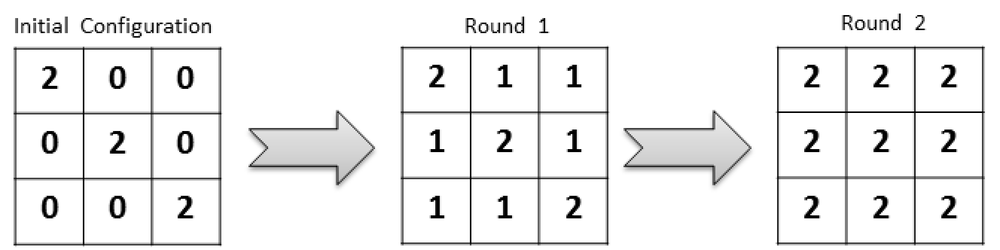
A ( $k,t$ )-dynamo is a $k$ -dynamo which reaches its final configuration within $t$ rounds, that is, $c_{v}(i)=k-1$ for each node $v\in V$ and $i\geq t.$ An example of ( $k,t$ )-dynamo, with $\lambda=1/2$ , is depicted in Figure 1. Given a graph $G$ , a set of weights $[k]$ , a threshold $\lambda$ , and an integer $t>0$ , we aim for a minimum weight ( $k,t$ )-dynamo.

Definition 2

A ( $k,t$ )-dynamo on a graph $G$ with threshold $\lambda$ is optimal if its weight is minimal among all the ( $k,t$ )-dynamos for the graph $G$ with threshold $\lambda$ .

Refer to caption — Figure 1: A ( $3,2$ )-dynamo on a $3\times 3$ Tori ( $\lambda=1/2$ ): Starting from the initial configuration (left), two rounds are needed to reach the final all-( $2$ )s configuration.

3 Time bounded dynamos

In this section we provide a lower bound on the weight of a ( $k,t$ )–dynamo and study the minimum value of $t$ for which an optimal ( $k,t$ )–dynamo coincides with a $k$ –dynamo.

3.1 Preliminary Results

Definition 3

Consider an undirected connected graph $G=(V,E)$ . Let $k\geq 2$ and $t\geq 1$ be integers and $0<\lambda\leq 1$ . An initial configuration ${\cal C}$ for $G$ is called ( $k,t$ )-simple-monotone if $V$ can be partitioned into $t+1$ sets ${X}_{-s},{X}_{-s+1},\ldots{X}_{k-1}$ (here $s=t-k+1$ ) where ${X}_{k-1}\neq\emptyset$ , and for each $v\in{X}_{i}$

(i) $c_{v}(0)=\max(i,0)$ ;

(ii) $v$ has at least $\lceil\lambda d(v)\rceil$ neighbours in $\bigcup_{j=i+1}^{k-1}{X}_{j}.$

Lemma 1

Any ( $k,t$ )-simple-monotone configuration for an undirected connected graph $G$ is a ( $k,t$ )-dynamo for $G$ .

Proof 1

We show that for each $i=-s,-s+1,\ldots,k-1$ (here $s=t-k+1$ ) and $j=0,\ldots,t$ and for each $u\in X_{i}$

c_{u}(j)=\left\{\begin{array}[]{l l}\min(j+i,k-1)&\text{if $j+i>0$}\\ 0&\text{otherwise.}\end{array}\right.

We prove this statement by induction on $i$ from $k-1$ back to $-s$ . For $i=k-1$ the nodes in $X_{k-1}$ have weight $k-1$ from the initial configuration and the statement is trivially true for each round $j$ .
Assume now that the statement is true for any $r>i$ . For each $u\in X_{i}$ , we know that $u$ has at least $\lceil\lambda d(v)\rceil$ neighbours which belong to $\bigcup_{r=i+1}^{k-1}{X}_{r}$ . By induction, each of this neighbor nodes, for each round $j$ has a weight greater or equal to $\min(j+i+1,k-1)$ if $j+(i+1)>0$ .

Hence, $u$ preserves its weight $c_{u}(j)=max(i,0)=0$ until it increases its weight at each round $j$ such that $j+(i+1)>1$ (i.e. $j+i>0$ ) and $c_{u}(j)<k-1$ ; as a result each node in ${X}_{i}$ has weight $\min(j+i,k-1)$ whenever $j+i>0$ , for each $j=0,1,\ldots,t$ .
The Lemma follows since at round $t$ , $i+j=i+t\geq-s+t=k-1>0$ . Hence, all the nodes will have weight $\min(i+t,k-1)=k-1.$ .

Lemma 2

Let $G=(V,E)$ be an undirected connected graph. There exists an optimal ( $k,t$ )-dynamo for $G$ which is a ( $k,t$ )-simple-monotone configuration for $G$ .

Proof 2

Let ${\cal C}$ be an optimal ( $k,t$ )-dynamo. Define a new configuration ${\cal C}^{\prime}$ as follows: Let $s=t-k+1$ , for $i=k-1,k-2,\ldots,-s$ , let ${X}_{i}$ be the set of nodes that, starting with configuration ${\cal C}$ , reaches permanently the weight $k-1$ at round $k-1-i$ , that is,

${X}_{i}=\{u\in V\ |\ c_{u}(k-2-i)\neq k-1,\hbox{ and }c_{u}(j)=k-1\hbox{ for each }j\geq k-1-i\}.$
In ${\cal C}^{\prime}$ , for each $u\in X_{i}$ set $c^{\prime}_{u}(0)=\max(i,0).$
Notice that since ${\cal C}$ is a $k$ -dynamo which converges into $t$ rounds, $\{{X}_{-s},{X}_{-s+1},\ldots,{X}_{k-1}\}$ is a partition of $V$ and ${X}_{k-1}\neq\emptyset$ . We now show that $w({\cal C}^{\prime})\leq w({\cal C})$ and ${\cal C}^{\prime}$ is a ( $k,t$ )-simple-monotone configuration for $G$ . Clearly,

(a)

for each index $i\leq 0,$ and for each $u\in{X}_{i},$ $c_{u}(0)\geq c^{\prime}_{u}(0)=0$ ;
(b)

for each $i>0$ and for each $u\in{X}_{i}$ we have $c_{u}(0)\geq c^{\prime}_{u}(0)=i$ (otherwise $u$ cannot reach the final weight $k-1$ by round $k-1-i$ , since the weight of a node increases by at most $1$ at each round).

By using (a) and (b) above we have that $w({\cal C}^{\prime})\leq w({\cal C})$ . It remains to show that ${\cal C}^{\prime}$ is a ( $k,t$ )-simple-monotone configuration for $G$ . By construction, ${\cal C}^{\prime}$ satisfies point (i) of Definition 3. Moreover, for each $u\in X_{i}$ , we know that $u$ in the configuration ${\cal C}$ reaches the weight $k-1$ at round $k-1-i$ . Hence at least $\lceil\lambda d(v)\rceil$ of its neighbors have weight $k-1$ at round $k-1-i-1=k-1-(i+1)$ , that is at least $\lceil\lambda d(v)\rceil$ of its neighbors belong to $\bigcup_{j=i+1}^{k-1}{X}_{j}$ . Hence, point (ii) of Definition 3 also holds.

3.2 A Lower Bound

Theorem 1

Consider an undirected connected graph $G=(V,E)$ and let $k\geq 2$ and $t\geq 1$ be integers. Any ( $k,t$ )-dynamo ${\cal C}$ , with $\lambda=1/2$ , has weight

w({\cal C})\geq\left\{\begin{array}[]{l l}\frac{|V|}{2\rho(\ell+s+1)+1}\times\left(k{-}1+\rho\ell(\ell{+}1)\right)\\ \ \ \ \ \text{ where }\ell=\left\lfloor\frac{\sqrt{(2\rho s+\rho+1)^{2}+4\rho(k-1)}-(2\rho s+\rho+1)}{2\rho}\right\rfloor&\text{if $t\geq k-1$}\\ \frac{|V|}{2\rho(\ell+s+1)+1}\times\left(k{-}1+\rho(\ell(\ell{+}1)-s(s{+}1))\right)\\ \ \ \ \ \text{ where }\ell=\left\lfloor\frac{\sqrt{4\rho(t+1)+(\rho-1)^{2}}-(2\rho s+\rho+1)}{2\rho}\right\rfloor&\text{otherwise,}\end{array}\right.

where $\rho$ is the ratio between the maximum and the minimum degree of the nodes in $V$ and $s=t-k+1$ .

Proof 3

By Lemma 2 we can restrict our attention to ( $k,t$ )-simple-monotone configurations for $G$ . Therefore, the set $V$ can be partitioned into $t+1$ subsets ${X}_{-s},{X}_{-s+1},\ldots,{X}_{k-1}$ where $s=t-k+1$ and for $i=-s,-s+1,\ldots,k-1$ , ${X}_{i}$ denotes the set of nodes whose weight at round $j$ is $\max(0,\min(j+i,k-1))$ . Henceforth, we denote the size of ${X}_{i}$ by ${x}_{i}$ and the sum of the degree of nodes in $A\subseteq V$ by $d(A)$ .
In order to prove the theorem, we first show that, for each $i=-s,-s+1,\ldots,k-2$ , it holds

{x}_{i}\leq 2\rho{x}_{k-1}.

(1)

Let $E(A,B)=|\{e=(u,v)\in E\ \colon\ u\in A\mbox{ and }v\in B\}|$ denote the number of edges between a node in $A$ and one in $B$ . Each node $v\in{X}_{i}$ must increase its weight for each round $r$ such that $0<r+i<k-1$ ; hence, at round $r=\max(-i+1,0)$ , node $v$ must have at least $\lceil d(v)/2\rceil$ neighbors which belong to $\bigcup_{j=i+1}^{k-1}{X}_{j}$ . Overall the number of edges between ${X}_{i}$ and $\bigcup_{j=i+1}^{k-1}{X}_{j}$ satisfies

E\left({X}_{i},\bigcup_{j=i+1}^{k-1}{X}_{j}\right)\geq\frac{d(X_{i})}{2}\geq\frac{|X_{i}|d_{min}}{2}=\frac{x_{i}d_{min}}{2},

(2)

where $d_{min}$ represents the minimum degree of a node in $G$ . Moreover, for each $i=-s,-s+1,\ldots,k-2$ , the number of edges between ${X}_{i}$ and $\bigcup_{j=i+1}^{k-1}{X}_{j}$ is

$\displaystyle E\left({X}_{i},\bigcup_{j=i+1}^{k-1}{X}_{j}\right)$	$\displaystyle\leq$	$\displaystyle\sum_{j=i+1}^{k-1}d({X}_{j})-2E\left({X}_{i+1},\bigcup_{j=i+1}^{k-1}{X}_{j}\right)-2E\left({X}_{i+2},\bigcup_{j=i+2}^{k-1}{X}_{j}\right)-\ldots$
		$\displaystyle\qquad\qquad\ldots-2E\left({X}_{k-2},{X}_{k-2}\cup{X}_{k-1}\right)-2E\left({X}_{k-1},{X}_{k-1}\right)$
	$\displaystyle\leq$	$\displaystyle\sum_{j=i+1}^{k-1}d({X}_{j})-2\left[E\left({X}_{i+1},\bigcup_{j=i+2}^{k-1}{X}_{j}\right)+E\left({X}_{i+2},\bigcup_{j=i+3}^{k-1}{X}_{j}\right)+\right.$
		$\displaystyle\qquad\qquad\left.\ldots+E({X}_{k-2},{X}_{k-1})\right]$
	$\displaystyle\leq$	$\displaystyle\sum_{j=i+1}^{k-1}d({X}_{j})-2\left[d({X}_{i+1})/2+d({X}_{i+2})/2+\ldots+d({X}_{k-2})/2\right]$
	$\displaystyle=$	$\displaystyle d({X}_{k-1})\leq d_{max}\|X_{k-1}\|=d_{max}x_{k-1},$

where $d_{max}$ is the maximum node degree of a node in $G$ . By this and (2), recalling that $\rho=d_{max}/d_{min}$ , we get (1).

Define now $y_{i}={x}_{i}/{x}_{k-1}$ . By (1), $0\leq y_{i}\leq 2\rho$ . Our goal is to minimize the weight function $w({\cal C})=\sum_{j=1}^{k-1}j{x}_{j}={x}_{k-1}\left((k-1)+\sum_{j=1}^{k-2}jy_{j}\right)$ with $|V|=\sum_{j=-s}^{k-1}{x}_{j}={x}_{k-1}\left(1+\sum_{j=-s}^{k-2}y_{j}\right).$ Hence, ${x}_{k-1}=\frac{|V|}{1+\sum_{j=-s}^{k-2}y_{j}}$ and we can write

w(C)=|V|\times\frac{k-1+\sum_{j=1}^{k-2}jy_{j}}{1+\sum_{j=-s}^{k-2}y_{j}}.

(3)

We distinguish now two cases depending on whether $t\geq k-1$ or $t<k-1$ .

Case I ( $t\geq k-1$ ): In this case, it is possible to show that the rightmost term of (3) is minimized when

y_{i}=\begin{cases}{2\rho}&{\hbox{ if }-s\leq i\leq\ell}\cr{0}&{\hbox{ if }\ell<i\leq k-2,}\end{cases}

(4)

where $\ell{=}\left\lfloor\frac{\sqrt{(2\rho s+\rho+1)^{2}+4\rho(k-1)}-(2\rho s+\rho+1)}{2\rho}\right\rfloor$ is the floor of the positive root of the equation $\rho i^{2}+(2\rho s{+}\rho{+}1)i-(k{+}1).$
Let $f(y_{-s},y_{-s+1},\ldots,y_{k-2})=\frac{k-1+\sum_{j=1}^{k-2}jy_{j}}{1+\sum_{j=-s}^{k-2}y_{j}}.$ This function is decreasing in $y_{i}$ for each $-s\leq i\leq 0$ . Hence, since $0\leq y_{j}\leq 2\rho$ for each $j$ ,

$f(y_{-s},y_{-s+1},\ldots,y_{0},y_{1},\ldots,y_{k-2})\geq f(2\rho,2\rho,\ldots,2\rho,y_{1},\ldots,y_{k-2}).$

Moreover, we show that the following two inequalities hold:

$\displaystyle f(2\rho,2\rho,\ldots,2\rho,y_{1},\ldots,y_{\ell},\ldots,y_{k-2})$	$\displaystyle\geq$	$\displaystyle f(2\rho,2\rho,\ldots,2\rho,y_{2},\ldots,y_{\ell},\ldots,y_{k-2})$	(5)
	$\displaystyle\geq$	$\displaystyle f(2\rho,2\rho,\ldots,2\rho,y_{3},\ldots,y_{\ell},\ldots,y_{k-2})$
	$\displaystyle\geq$	$\displaystyle...$
	$\displaystyle\geq$	$\displaystyle f(2\rho,2\rho,\ldots,2\rho,y_{\ell+1},\ldots y_{k-2})$

$\displaystyle\vskip-11.38092ptf(2\rho,2\rho,\ldots,2\rho,y_{\ell+1},\ldots y_{k-2})$	$\displaystyle\geq$	$\displaystyle f(2\rho,2\rho,\ldots,2\rho,y_{\ell+1},\ldots y_{k-3},0)$	(6)
	$\displaystyle\geq$	$\displaystyle f(2\rho,2\rho,\ldots,2\rho,y_{\ell+1},\ldots y_{k-4},0,0)$
	$\displaystyle\geq$	$\displaystyle\ldots$
	$\displaystyle\geq$	$\displaystyle f(2\rho,2\rho,\ldots,2\rho,0,0,\ldots,0).\vskip-5.69046pt$

We first prove (5). Each inequality in (5) is obtained by considering the following one for some $i\leq\ell$ (recalling that $\ell$ is the floor of the positive root of the equation $\rho i^{2}+(2\rho s{+}\rho{+}1)i-(k{+}1)$ )

\displaystyle f(2\rho,\ldots,2\rho,y_{i},\ldots,y_{k-2}){=}\frac{A{+}iy_{i}}{B{+}y_{i}}{\geq}\frac{A{+}2\rho i}{B{+}2\rho}{=}f(2\rho,\ldots,2\rho,y_{i+1},\ldots,y_{k-2})\vskip-5.69046pt

(7)

where $A=k{-}1+\sum_{j=i+1}^{k-2}jy_{j}+\rho i(i-1)$ and $B=1+\sum_{j=i+1}^{k-2}y_{j}+2\rho(i+s).$

We notice that (7) is satisfied whenever $y_{i}(A-iB)\leq 2\rho(A-iB)$ and that for $i\leq\ell$

$\displaystyle A-iB$	$\displaystyle=$	$\displaystyle k-1+\sum_{j=i+1}^{k-2}jy_{j}+\rho i(i-1)-i\left(1+\sum_{j=i+1}^{k-2}y_{j}+2\rho(i+s)\right)$
	$\displaystyle=$	$\displaystyle k-1+\sum_{j=i+1}^{k-2}(j-i)y_{j}+\rho i^{2}-\rho i-i-2\rho i^{2}-2\rho is$
	$\displaystyle\geq$	$\displaystyle-\rho i^{2}-(2\rho s+\rho+1)i+k-1\geq 0.$

Hence, (7) and consequently (5) are satisfied. In order to get (6), we show that for each $i>\ell$

	$\displaystyle\hskip-14.22636ptf(2\rho,\ldots,2\rho,y_{\ell+1},\ldots,y_{i},0,\ldots,0)$	$\displaystyle{=}$	$\displaystyle\frac{C{+}iy_{i}}{D{+}y_{i}}$		(8)
		$\displaystyle{\geq}$	$\displaystyle\frac{C}{D}{=}f(2\rho,\ldots,2\rho,y_{\ell+1},\ldots,y_{i-1},0,\ldots,0)$		(8)

where $C=k{-}1+\sum_{j=\ell+1}^{i-1}jy_{j}+\rho\ell(\ell+1)$ and $D=1+\sum_{j=\ell+1}^{i-1}y_{j}+2\rho(s{+}\ell{+}1)$ .

Since (8) is satisfied whenever $y_{i}(C-iD)\leq 0$ and since now $i>\ell$ we get

$\displaystyle\vskip-5.69046ptC-iD$	$\displaystyle=$	$\displaystyle k-1+\sum_{j=\ell+1}^{i-1}jy_{j}+\rho\ell(\ell+1)-i\left(1+\sum_{j=\ell+1}^{i-1}y_{j}+2\rho(s+\ell+1)\right)$
	$\displaystyle\leq$	$\displaystyle k-1+\rho\ell^{2}+\rho\ell-(\ell+1)-2\rho(\ell+1)s-2\rho(\ell+1)\ell-2\rho(\ell+1)$
	$\displaystyle=$	$\displaystyle-\rho\ell^{2}-(2\rho s+3\rho+1)\ell+k-2\rho s-2\rho-2\leq 0.$

Hence, (8) and consequently (6) are satisfied. Summarizing, we have that the minimizing values are

{x}_{i}=\left\{\begin{array}[]{l l}\frac{|V|}{1+\sum_{j=-s}^{k-2}y_{j}}=\frac{|V|}{2\rho(\ell+s+1)+1},&\quad\text{for $i=k-1$}\\ 2\rho x_{k-1}=\frac{2\rho|V|}{2\rho(\ell+s+1)+1}&\quad\text{for $i=-s,-s+1,\ldots,\ell$}\\ 0&\quad\text{otherwise.}\end{array}\right.

Therefore,

\displaystyle\sum_{j=1}^{k-1}j{x}_{j}

\displaystyle=

\displaystyle\frac{|V|}{2\rho(\ell{+}s{+}1){+}1}\left(k{-}1{+}2\rho\sum_{j=1}^{\ell}j\right)=\frac{|V|}{2\rho(\ell{+}s{+}1){+}1}\times\left(k{-}1{+}\rho\ell(\ell{+}1)\right),

and we can conclude that $w({\cal C})\geq\frac{|V|}{2\rho(\ell+s+1)+1}\times\left(k-1+\rho\ell(\ell+1)\right)$ , when $t\geq k-1$ .

Case II ( $t<k-1$ ): The proof of this case is left to the reader.

Corollary 1

Consider an undirected connected $d$ -regular graph $G=(V,E)$ . Let $k\geq 2$ and $t\geq 1$ be integers. Any ( $k,t$ )-dynamo ${\cal C}$ , with $\lambda=1/2$ , has weight

w({\cal C})\geq\left\{\begin{array}[]{l l}\frac{|V|}{2\ell+2s+3}\times\left(k{-}1{+}\ell(\ell{+}1)\right)\text{ where }\ell=\lfloor\sqrt{t{+}1{+}s^{2}{+}s}\rfloor{-}(s{+}1)&\text{if $t\geq k-1$}\\ \\ \frac{|V|}{2\ell+2s+3}\times\left(k{-}1{+}\ell(\ell{+}1)-s(s{+}1)\right)\text{ where }\ell=\lfloor\sqrt{t{+}1}\rfloor{-}(s{+}1)&\text{otherwise,}\end{array}\right.

where $s=t-k+1.$

We are now able to answer the question: Which is the smallest value of $t$ such that the optimal dynamo contains only two weights? By analyzing the value of $\ell$ in the case $t\geq k-1$ we have that whenever $t>\frac{k(2\rho+1)-2\rho-4}{2\rho}$ then $\ell=0$ , hence only the weights $0$ and $k-1$ will appear in the optimal configuration. When $\rho=1$ (i.e., on regular graphs) one has $t>\frac{3}{2}k-3$ .

Remark 1

Our result generalizes the one in [10] with $k=2$ . Indeed, when $t\geq k-1=1$ by the above consideration we get $t>\frac{3}{2}k-3=0$ and $\ell=0$ . Hence, $w({\cal C})\geq\frac{|V|}{2s+3}\times(k-1)=\frac{|V|}{2t+1}$ .

Theorem 2

Let $G=(V,E)$ be an undirected connected graph, if $t$ is sufficiently large, then:

(i): any optimal $(k,t)$ -dynamo contains only the weights $0$ and $k-1$ ;
(ii): let $k\geq 2$ be an integer and ${\cal C}_{2}$ a 2–dynamo on $G$ . Let ${\cal C}_{k}$ be obtained from ${\cal C}_{2}$ by replacing the weight $1$ with the weight $k-1$ . If ${\cal C}_{2}$ is an optimal $2$ -dynamo then ${\cal C}_{k}$ is an optimal $k$ -dynamo. Moreover, $w({\cal C}_{k})=w({\cal C}_{2})\times(k-1)$ and $t({\cal C}_{k})=t({\cal C}_{2})+k-2$ (where $t({\cal C})$ is the time needed to reach the final configuration).

Proof omitted.

4 Building ( $k,t$ )-dynamo

In this section we provide several optimal (or almost optimal) ( $k,t$ )-dynamo constructions for Rings and Tori ( $\lambda=1/2$ ) and Cliques (any $\lambda$ ).

4.1 Rings

A $n$ -node ring ${\cal R}_{n}$ consists of $n$ nodes and $n-1$ edges, where for $i=0,1,\ldots,n-1$ each node $v_{i}$ is connected with $v_{(i-1)\bmod n}$ and $v_{(i+1)\bmod n}$ .

A necessary condition for ${\cal C}({\cal R}_{n},k)$ to be a $k$ -dynamo ( $\lambda\leq 1/2$ ) is that at least one node of ${\cal R}_{n}$ is weighted by $k-1$ . This condition is also sufficient.

Theorem 3

An optimal $k$ -dynamo ( $\lambda\leq 1/2$ ) ${\cal C}({\cal R}_{n},k)$ has weight $w({\cal C}({\cal R}_{n},k))=(k-1)$ , and it reaches its final configuration within $t=k-2+\lceil{\frac{n-1}{2}}\rceil$ rounds.

A ( $k,t$ )-dynamo ( $\lambda=1/2$ ) for a ring ${\cal R}_{n}$ is obtained by the following partition of $V$ which defines the initial configuration (see Figure 2) ${\cal C}({\cal R}_{n},k,t)$ : for $i=0,1,\ldots,n$ ,

\forall v_{i}\in{\cal R}_{n},\ \ v_{i}\in\left\{\begin{array}[]{l l}{X}_{k-1}&\quad\text{if $j=0$}\\ {X}_{\ell+1-j}&\quad\text{if $1\leq j\leq\ell+s+1$}\\ {X}_{j-\ell-2s-2}&\quad\text{if $\ell+s+2\leq j\leq 2\ell+2s+2$}\end{array}\right.

where $s=t-k+1,$ $j=i\bmod(2\ell+2s+3)$ and $\ell=\lfloor\sqrt{t+1+s^{2}+s}\rfloor-(s+1)$ if $t\geq k-1$ and $\ell=\lfloor\sqrt{t+1}\rfloor-(s+1)$ otherwise.

Theorem 4

(i) The configuration ${\cal C}({\cal R}_{n},k,t)$ is a ( $k,t$ )-dynamo for any value of $n$ , $\lambda=1/2$ , $k\geq 2$ and $t\geq 1$ . (ii) The weight of ${\cal C}({\cal R}_{n},k,t)$ is

w({\cal C}({\cal R}_{n},k,t))\leq\left\{\begin{array}[]{l l}\left\lceil\frac{n}{2\ell+2s+3}\right\rceil\left(k{-}1+\ell(\ell{+}1)\right)&\text{if $t\geq k-1$}\\ \text{ \ \ \ \ where }\ell=\lfloor\sqrt{t+1+s^{2}+s}\rfloor-(s{+}1)\\ \left\lceil\frac{n}{2\ell+2s+3}\right\rceil\left(k{-}1+\ell(\ell{+}1)-s(s{+}1)\right)&\text{otherwise}\\ \text{ \ \ \ \ where }\ell=\lfloor\sqrt{t+1}\rfloor-(s{+}1)\end{array}\right.

Proof 4

(i) By construction ${\cal C}({\cal R}_{n},k,t)$ is ( $k,t$ )-simple-monotone, hence by Lemma 1, ${\cal C}({\cal R}_{n},k,t)$ is a ( $k,t$ )-dynamo. (ii) There are two cases to consider: if $t\geq k-1$ , then starting from $v_{0}$ each set of $2\ell+2s+3$ nodes weights $k-1+2\sum_{i=1}^{\ell}i=k-1+\ell(\ell+1)$ . Then the weight of ${\cal C}({\cal R}_{n},k,t)$ is smaller than the weight of ${\cal C}({\cal R}_{\overline{n}},k,t)$ where $\overline{n}=\lceil\frac{n}{2\ell+2s+3}\rceil\times(2\ell+2s+3).$ Hence, $w({\cal C}({\cal R}_{n},k,t))\leq w({\cal C}({\cal R}_{\overline{n}},k,t))=\left\lceil\frac{n}{2\ell+2s+3}\right\rceil\left(k{-}1+\ell(\ell{+}1)\right)$ . Similarly for $t<k-1.$

By Corollary 1 and Theorem 4 we have the following Corollary.

Corollary 2

When $n/(2\ell+2s+3)$ is integer, ${\cal C}({\cal R}_{n},k,t)$ is an optimal ( $k,t$ )-dynamo.

4.2 Tori

A $n\times m$ -node tori ${\cal T}_{n,m}$ consists of $n\times m$ nodes and $2(n\times m)$ edges, where for $i=0,1,\ldots,n-1$ and $j=0,1,\ldots,m-1$ , each node $v_{i,j}$ is connected with four nodes: $v_{i,(j-1)\bmod m}$ , $v_{i,(j+1)\bmod m}$ , $v_{(i-1)\bmod n,j}$ and $v_{(i+1)\bmod n,j}$ .

A ( $k,t$ )-dynamo ( $\lambda=1/2$ ) for ${\cal T}_{2\ell+2s+3,2\ell+2s+3}$ is obtained by weighting diagonals with the same order defined for dynamos on rings. Specifically, the configuration
${\cal C}({\cal T}_{2\ell+2s+3,2\ell+2s+3},k,t)$ is defined by the partition of $V$ described as follows, let $D_{i}=\{v_{a,b}\ :\ i=(b-a)\bmod(2\ell+2s+3)\}$ denote the $i$ -th diagonal of ${\cal T}_{2\ell+2s+3,2\ell+2s+3}$ , for $i=0,1,\ldots,2\ell+2s+2,$

\forall v\in D_{i},\ \ v\in\left\{\begin{array}[]{l l}{X}_{k-1}&\quad\text{if $i=0$}\\ {X}_{\ell+1-i}&\quad\text{if $1\leq i\leq\ell+s+1$}\\ {X}_{i-\ell-2s-2}&\quad\text{if $\ell+s+2\leq i\leq 2\ell+2s+2,$}\end{array}\right.

where $s=t-k+1,$ $\ell=\lfloor\sqrt{t+1+s^{2}+s}\rfloor-(s+1)$ if $t\geq k-1$ and $\ell=\lfloor\sqrt{t+1}\rfloor-(s+1)$ otherwise. Some examples are depicted in Figure 3.

Theorem 5

The configuration ${\cal C}({\cal T}_{2\ell+2s+3,2\ell+2s+3},k,t)$ is an optimal ( $k,t$ )-dynamo for any $k\geq 2$ , $t\geq 1$ and $\lambda=1/2$ .

Proof 5

Let ${\cal C}={\cal C}({\cal T}_{2\ell+2s+3,2\ell+2s+3},k,t)$ . By construction ${\cal C}$ is ( $k,t$ )-simple-monotone, hence by Lemma 1, it is a ( $k,t$ )-dynamo. To show its optimality we distinguish two cases. If $t\geq k-1,$ each row (resp. each column) corresponds to ${\cal C}({\cal R}_{2\ell+2s+3},k,t)$ and its weight is $k-1+\ell(\ell+1)$ . Overall, $w({\cal C})=(2\ell+2s+3)\times\left(k-1+\ell(\ell+1)\right)$ that matches the bound in Corollary 1. Similarly for $t<k-1$ .

A ( $k,t$ )-dynamo for ${\cal T}_{n,m}$ is obtained by building a grid $\lceil\frac{n}{2\ell+2s+3}\rceil\times\lceil\frac{m}{2\ell+2s+3}\rceil$ , where each cell is filled with a configuration ${\cal C}({\cal T}_{2\ell+2s+3,2\ell+2s+3},k,t)$ defined above. Then, the exceeding part is removed and the last row and the last column are updated. In particular, for each column (resp. row), if the removed part contains a $k-1$ , then the element in the last row (resp. column) is given the value $k-1$ (see Figure 4). We call this configuration ${\cal C}({\cal T}_{n,m},k,t)$ .

Theorem 6

(i) ${\cal C}({\cal T}_{n,m},k,t)$ is a ( $k,t$ )-dynamo for any value of $n$ , $m$ , $\lambda=1/2$ , $k\geq 2$ and $t\geq 1$ .
(ii) The weight of ${\cal C}({\cal T}_{n,m},k,t)$ is

w({\cal C}({\cal T}_{n,m},k,t))\leq\left\{\begin{array}[]{l l}\lceil\frac{n}{2\ell{+}2s{+}3}\rceil\lceil\frac{m}{2\ell{+}2s{+}3}\rceil(2\ell{+}2s{+}3)\left(k{-}1{+}\ell(\ell{+}1)\right)&\text{if $t\geq k-1$}\\ \ \ \ \text{ where }\ell=\lfloor\sqrt{t{+}1{+}s^{2}{+}s}\rfloor{-}(s{+}1)\\ \lceil\frac{n}{2\ell{+}2s{+}3}\rceil\lceil\frac{m}{2\ell{+}2s{+}3}\rceil(2\ell{+}2s{+}3)\left(k{-}1{+}\ell(\ell{+}1){-}s(s{+}1)\right)&\text{otherwise}\\ \ \ \ \text{ where }\ell=\lfloor\sqrt{t{+}1}\rfloor{-}(s{+}1).\end{array}\right.

Proof 6

(i) By construction ${\cal C}({\cal T}_{n,m},k,t)$ is ( $k,t$ )-simple-monotone (cfr. Figure 4), hence by Lemma 1, ${\cal C}({\cal T}_{n,m},k,t)$ is a ( $k,t$ )-dynamo.
(ii) The grid contains $\lceil\frac{n}{2\ell+2s+3}\rceil\times\lceil\frac{m}{2\ell+2s+3}\rceil$ cells. If $t\geq k-1$ , each cell has weight
$w({\cal C}({\cal T}_{2\ell+2s+3,2\ell+2s+3},k,t))=(2\ell+2s+3)\times\left(k-1+\ell(\ell+1)\right).$
Moreover, the nodes that change their weight take the weight of a removed element. Hence, the weight of ${\cal C}({\cal T}_{n,m},k,t)$ is upper bounded by the weight of the full grid which is $\lceil\frac{n}{2\ell+2s+3}\rceil\times\lceil\frac{m}{2\ell+2s+3}\rceil\times w({\cal C}({\cal T}_{2\ell+2s+3,2\ell+2s+3},k,t))$ . Similarly for $t<k-1$ .

By Corollary 1 and Theorem 6 we have the following Corollary.

Corollary 3

If both $n$ and $m$ are multiples of $2\ell+2s+3$ , ${\cal C}({\cal T}_{n,m},k,t)$ is an optimal ( $k,t$ )-dynamo.

4.3 Cliques

Let $K_{n}$ be the clique on $n$ nodes. A necessary condition for a $k$ -dynamo ${\cal C}(K_{n},k)$ is that $\lceil\lambda(n-1)\rceil$ nodes are weighted by $k-1$ . The condition is also sufficient and if the remaining $\lfloor\lambda(n-1)\rfloor$ nodes are weighted by $0$ , the $k$ -dynamo is optimal and reaches its final configuration within $t=k-1$ rounds. So, when $t\geq k-1$ the optimal configuration is obtained by weighting $\lceil\lambda(n-1)\rceil$ nodes by $k-1$ and the remaining nodes by $0$ . For $t<k-1$ , an optimal ( $k$ , $t$ )-dynamo is obtained by assigning weight $k-t-1$ to all the non- $k-1$ weighted nodes. Clearly this configuration is optimal, if we assign a weight smaller than $k-t-1$ to a node $v$ , then $v$ can not reach the weight $k-1$ within $t$ rounds. Therefore:

Theorem 7

Let $K_{n}$ be the clique on $n$ nodes. An optimal ( $k$ , $t$ )-dynamo ${\cal C}(K_{n},k,t)$ has weight
$w({\cal C}(K_{n},k,t))=(k-1)\times\lceil\lambda(n-1)\rceil+\max(k-t-1,0)\times\lfloor\lambda(n-1)\rfloor$ .

5 Conclusion and Open Problems

In this work we studied multivalued dynamos with respect to both weight and time. We derived lower bounds on the weight of ( $k,t$ )-dynamo and provided constructive tight upper bounds for rings, tori and cliques. Several dimensions of the problem remain unexplored, different updating rules with could be addressed, as for instance the case of reversible rules. Finally, the behavior of this protocol on different topologies such as small world [20], scale-free [1], and time-varying networks [6].

Acknowledgments.

We would like to thank Ugo Vaccaro for many stimulating discussions and the anonymous referees whose helpful comments allowed to significantly improve the presentation of their work.

References

[1] A. L. Barabasi and R. Albert. Emergence of scaling in random networks. Science (New York, N.Y.), 286(5439):509–512, October 1999.
[2] J.C. Bermond, J. Bond, D. Peleg, and S. Perennes. Tight bounds on the size of 2-monopolies. In SIROCCO, pp. 170-179, 1996.
[3] J.C. Bermond, J. Bond, D. Peleg, and S. Perennes. The power of small coalitions in graphs. Discrete Applied Mathematics, 127(3):399–414, 2003.
[4] J.C. Bermond, L. Gargano, A.A. Rescigno, and U. Vaccaro. Fast Gossiping by Short Messages. SIAM J. on Computing, 27(4):917–941, 1998.
[5] S. Brunetti, E. Lodi, and W. Quattrociocchi. Dynamic monopolies in colored tori. In IPDPS Workshops, pp. 626-631, 2011.
[6] A. Casteigts, P. Flocchini, W. Quattrociocchi, and N. Santoro. Time-varying graphs and dynamic networks. International Journal of Parallel, Emergent and Distributed Systems, 0(0):1–22, 2012.
[7] N. Chen. On the approximability of influence in social networks. SIAM J. Discret. Math., 23:1400–1415, September 2009.
[8] P. Domingos and M. Richardson. Mining the network value of customers. In KDD ’01: Proceedings of the seventh ACM SIGKDD international conference on Knowledge discovery and data mining, pp. 57–66, New York, NY, USA, 2001.
[9] D. Easley and J. Kleinberg. Networks, Crowds, and Markets: Reasoning About a Highly Connected World. Cambridge University Press, 2010.
[10] P. Flocchini, R. Královič, P. Ružička, A. Roncato, and N. Santoro. On time versus size for monotone dynamic monopolies in regular topologies. J. of Discrete Algorithms, 1(2):129–150, 2003.
[11] M. Granovetter. Economic action and social structure: the problem of embeddedness. American Journal of Sociology, 91, 1985.
[12] D. Kempe, J. Kleinberg, and E. Tardos. Maximizing the spread of influence through a social network. In KDD ’03: Proceedings of the ninth ACM SIGKDD international conference on Knowledge discovery and data mining, pp. 137–146, New York, NY, USA, 2003. ACM.
[13] T. Kulich. Dynamic monopolies with randomized starting configuration. Theor. Comput. Sci., 412(45):6371–6381, 2011.
[14] N. Linial, D. Peleg, Y. Rabinovich, and M. Saks. Sphere packing and local majorities in graphs. In ISTCS IEEE Computer Soc. Press, pp. 141-149, 1993.
[15] S. Mishra and S.B. Rao. Minimum monopoly in regular and tree graphs. Electronic Notes in Discrete Mathematics, 15(0):126, 2003.
[16] A. Nayak, L. Pagli, and N. Santoro. Efficient construction of catastrophic patterns for vlsi reconfigurable arrays with bidirectional links. In ICCI, pp. 79-83, 1992.
[17] D. Peleg. Size bounds for dynamic monopolies. Discrete Applied Mathematics, 86(2–3):263–273, 1998.
[18] D. Peleg. Local majorities, coalitions and monopolies in graphs: a review. Theor. Comput. Sci., Volume 282, Issue 2:231�257, 2002.
[19] T. W. Valente. Network models of the diffusion of innovations. Hampton Press, 1995.
[20] D.J. Watts. Small Worlds: The Dynamics of Networks Between Order and Randomness. Princeton University Press, 1999.