Gluon- and Quark-Jet Multiplicities with NNNLO and NNLL Accuracy
Abstract
We present a new approach to consider and include both the perturbative and the non-perturbative contributions to the multiplicities of gluon and quark jets. Thanks to this new method, we have included for the first time new contributions to these quantities obtaining next-to-next-to-leading-logarithmic resummed formulas. Our analytic expressions depend on two non-perturbative parameters with a clear and simple physical interpretation. A global fit of these two quantities shows how our results solve a longstanding discrepancy in the theoretical description of the data.
pacs
12.38.Cy,12.39.St,13.66.Bc,13.87.FhCollisions of particles and nuclei at high energies usually produce many hadrons. In quantum chromodynamics (QCD) their production is due to the interactions of quarks and gluons and to test it as a theory of strong interactions, the transition from a description based in terms of quarks and gluons to the hadrons observed in experiments is always needed. The production of hadrons is a typical process where non-perturbative phenomena are involved. However, the hypothesis of local parton-hadron duality assumes that parton distributions are simply renormalized in the hadronization process without changing their shape [1], allowing perturbative QCD to make predictions. The simplest observables of this kind are gluon and quark multiplicities and which represent the number of hadrons produced in a gluon and a quark jet respectively. In the framework of the generating-functional approach in the modified leading logarithmic approximation [2], several studies of the multiplicities have been performed [3, 4, 5]. In such studies, the ratio is at least 10% higher than the data or it has a slope too small. Good agreement with the data has been achieved in Ref. [6] where recoil effects are included. Nevertheless in Ref. [6] a constant offset to be fitted to the quark and gluon multiplicities has been introduced, while the authors of Ref. [7] suggested that other, better motivated possibilities should be studied.
In this Letter, we study such a possibility inspired by the new formalism that has recently been proposed in Ref. [8]. Thanks to very recent new results in small- timelike resummation obtained in Ref. [9], we are able to reach the next-to-next-to-leading-logarithmic (NNLL) accuracy level. A purely perturbative and analytic prediction has been already attempted in Ref. [7] up to the third order in the expansion parameter i.e. , where paradoxically the quark multiplicity and the ratio are not well described even if the behavior of the perturbative expansion is very good. Our new resummed results that we present here are a generalization of what was obtained in Ref. [7] and represent also a solution to this apparent paradox.
We consider the standard Mellin-space moments of the coupled gluon-singlet system whose evolution in the scale is governed in QCD by the Dokshitzer-Gribov-Lipatov-Altarelli-Parisi equations:
| (1) |
The timelike splitting functions can be computed perturbatively in the strong coupling constant:
| (2) |
where with being the usual Mellin conjugate variable to the fraction of longitudinal momentum . The functions with appearing in Eq.(2) in the scheme can be found in Refs. [10, 11, 12] through next-to-next-to-leading order (NNLO) and in Refs. [13, 14, 9] through the NNLL.
In general it is not possible to diagonalize Eq.(1) because the contributions to the splitting function matrix do not commute at different orders. It is, therefore, convenient (see e.g. Ref. [15]) to introduce a new basis, called plus-minus basis where the LO splitting matrix is diagonal with eigenvalues and . We define such a change of basis according to the following transformation of the gluon and the singlet fragmentation functions in Mellin space:
| (3) |
where
| (4) |
The general solution to Eq.(1) can be formally written as
| (5) |
where denotes the path ordering with respect to and
| (6) |
Now making the following ansatz:
| (7) |
where
| (8) |
is the all-order diagonal part of the splitting matrix in the plus-minus basis and is a matrix in the same basis with a perturbative expansion of the form:
| (9) |
we obtain that
| (10) |
where evolves like a “plus” component, evolves like a “minus” component, and
| (11) |
Here is a renoramlization group exponent which is given by
| (12) |
with
| (13) | |||||
We recall that
| (14) |
where , and in QCD and is the number of active flavors. In Eq.(11) are perturbative functions containing off-diagonal terms of beyond the LO and the normalization factors satisfy the following conditions:
| (15) |
We note that differ from starting at higher orders [15]. In the following, we collect the resummed formulas. Details of the calculation will be presented elsewhere [16].
After the resummation is perfomed for in Eq.(8) thanks to the results obtained in Refs. [17, 18, 9], we find for the first Mellin moment () at NNLL:
| (16) |
where
| (17) |
and
| (18) | |||||
with . Now we can perform the integration in Eq.(12) up to the NNLL to obtain that
| (19) | |||
| (20) | |||
| (21) |
where
| (22) |
We are now ready to define the avarage multiplicities in our formalism:
| (23) |
with for the gluon and quark multiplicities, respectively. From Eqs.(11) and (15) we have that
| (24) |
and
| (25) |
Using these definitions, it is convenient to write for the gluon and quark multiplicities in general:
| (26) |
For the coefficients of the renormalization group exponents, we clearly have the following simple relations at the lowest order in
| (27) |
with . One would like to include higher-order corrections to Eq.(27). However, this is highly non-trivial because the general perturbative structures of the functions and , whose knowledge is required for the resummation, are not known. Fortunatly, general assumptions and approximations can be made to improve them. Firstly, it is a well known fact that the plus components by themselves represent the dominant contributions for both the gluon and the quark multiplicities (see e.g. Refs. [19, 20]). Secondly, Eq.(25) tells us that is suppressed with respect to , because . These two facts suggest us that to keep even at higher orders should still represent a good approximation. Then we notice that higher-order corrections to and just represent a redefinition of apart from running coupling effects starting at order . Therefore we assume that these corrections can be neglected. Now we can finally discuss higher-order corrections to , which represents the ratio of the pure plus components. Accordingly, we can intepret the result in Eq.(5) of Ref. [7] as higher-order corrections to Eq.(24). This interpretation is explicitly confirmed up to order in Chapter 7 of Ref. [2], where also the same set of equations used in the computation of Ref. [7] are obtained. Further arguments to support it and its scheme dependence will be discussed in Ref. [16]. We denote the approximation in which Eqs.(19,27) are used as and the one in which in Eq.(27) is replaced by the result of Eq.(5) in Ref. [7] up to order as . That this last one is actually a good approximation will be shown below.
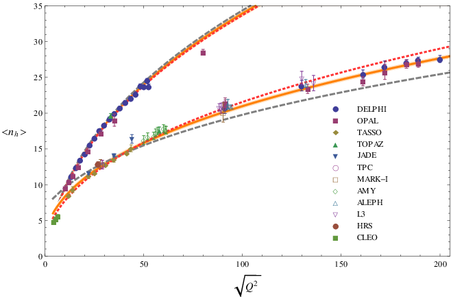

In both approximations considered we can summarize the main theoretical result of this Letter in the following way
| (28) | |||
| (29) |
for the multiplicities, and
| (30) | |||
for the gluon-quark multiplicity ratio. Equations (28,29) depend only on two parameters, and , with a simple physical interpretation: they are just the gluon and the quark multiplicities at the arbitrary scale .
We have performed a global fit of our resummed formulas, Eqs.(28,29), to the experimental data to extract the values of and . With , the result of the fit is given by
| (31) |
in the case and by
| (32) |
in the case in agreement with the experimental values within the errors. However, the C.L. error in the case is much smaller reflecting a much better fit to the data at all energies. Indeed, per degree of freedom we obtain in the case, while we have in the case. In our analysis, we have used the next-to-leading order solution for the running coupling according to Eq.(13) with and . We have checked that varying the arbitrary scale does not change the resulting value of as expected and that moving from LL to NNLL the renormalization scale dependence is strongly reduced.
In Fig.1 we plot the gluon and quark multiplicities according to Eqs.(26,28,29) using the fitted parameters given in Eqs.(31,32). Using the data selection of Ref. [21], the measurements are taken from Refs. [21, 22, 23, 24] for the gluon multiplicity and from Refs. [25, 26] and references therein for the quark multiplicity. The result of a fit where the normalization coefficients are assumed constant without any additional constraint is also plotted showing that is indeed a good approximation. To check the consistency of the data sets, we have used Eq.(30) together with the result of the fit from the gluon and quark multiplicities in Eqs.(31) and (32) to predict the gluon-quark multiplicity ratio. The result together with the corresponding data are shown in Fig.2. The data are taken from Refs. [27, 28, 26, 22, 29, 30, 21, 25] and references therein, covering essentially all available measurements. One can see that the data do not agree very well at small scales, an isssue that will be discussed elsewhere [16].
As concluding remarks we remind here that the main problem in describing the data was that the theory failed badly in the description of the data for the gluon and the quark jets simultaneously (or equivalently for the ratio ) even if the perturbative series seems to converge very well. We have shown in this Letter that our result solves this problem explaining the discrepancy of the results with the data obtained in Ref. [7] as due to the absence of the singlet “minus” component governed by in Eqs.(29) and (30). This component is included here for the first time. The most natural possible future improvement consists in including corrections of next-to-leading order or beyond to . Our generalized result depends on two parameters, which represent our initial condition. They have been fixed performing a fit and have a simple physical meaning because they just represent the gluon and the quark multiplicity at a certain arbitrary scale . We hope that additional measurements of these observables will come from the LHC to test our results on a much wider energy range.
We kindly thank A. Vogt and G. Kramer for valuable discussions. The work of A.V.K. was supported in part by the Heisenberg-Landau program and the Russian Foundation for Basic Research RFBR through Grant No. 11–02–01454–a. This work was supported in part by the German Federal Ministry for Education and Research BMBF through Grant No. 05H12GUE, by the German Research Foundation DFG through Grant No. KN 365/5-3, and by the Helmholtz Association HGF through the Helmholtz Alliance Ha 101 Physics at the Terascale.
References
- [1] Y. I. Azimov, Y. L. Dokshitzer, V. A. Khoze, and S. I. Troyan, Z. Phys. C27, 65 (1985).
- [2] Y. L. Dokshitzer, V. A. Khoze, A. H. Mueller, and S. I. Troian , Basics of Perturbative QCD(Frontiers, Gif-sur-Yvette, France, 1991), p.274.
- [3] E. D. Malaza and B. R. Webber, Nucl. Phys. B267, 702 (1986).
- [4] S. Catani, Y. L. Dokshitzer, F. Fiorani, and B. R. Webber, Nucl. Phys. B377, 445 (1992).
- [5] S. Lupia and W. Ochs, Phys. Lett. B418, 214 (1998), eprint hep-ph/9707393.
- [6] P. Eden and G. Gustafson, JHEP 09, 015 (1998), eprint hep-ph/9805228.
- [7] A. Capella, I. M. Dremin, J. W. Gary, V. A. Nechitailo, and J. Tran Thanh Van, Phys. Rev. D61, 074009 (2000), eprint hep-ph/9910226.
- [8] P. Bolzoni (2012), eprint 1206.3039.
- [9] C.-H. Kom, A. Vogt, and K. Yeats (2012), eprint 1207.5631.
- [10] M. Gluck, E. Reya, and A. Vogt, Phys. Rev. D48, 116 (1993).
- [11] S. Moch and A. Vogt, Phys. Lett. B659, 290 (2008), eprint 0709.3899.
- [12] A. A. Almasy, A. Vogt, and S. Moch (2011), eprint 1107.2263.
- [13] A. Vogt, JHEP 10, 025 (2011), eprint 1108.2993.
- [14] S. Albino, P. Bolzoni, B. A. Kniehl, and A. V. Kotikov, Nucl. Phys. B855, 801 (2012), eprint 1108.3948.
- [15] A. J. Buras, Rev. Mod. Phys. 52, 199 (1980).
- [16] P. Bolzoni, B. A. Kniehl, and A. Kotikov (to be published).
- [17] A. H. Mueller, Phys. Lett. B104, 161 (1981).
- [18] J. B. Gaffney and A. H. Mueller, Nucl. Phys. B250, 109 (1985).
- [19] M. Schmelling, Phys.Scripta 51, 683 (1995).
- [20] I. M. Dremin and J. W. Gary, Phys. Rept. 349, 301 (2001), eprint hep-ph/0004215.
- [21] J. Abdallah et al. (DELPHI Collaboration), Eur.Phys.J. C44, 311 (2005), eprint hep-ex/0510025.
- [22] G. Abbiendi et al. (OPAL Collaboration), Eur. Phys. J. C11, 217 (1999), eprint hep-ex/9903027.
- [23] K. Nakabayashi et al. (TOPAZ Collaboration), Phys.Lett. B413, 447 (1997).
- [24] G. Abbiendi et al. (OPAL Collaboration), Eur.Phys.J. C37, 25 (2004), eprint hep-ex/0404026.
- [25] M. Siebel (2003), PHD thesis,Bergische Universita¨t Wuppertal [Report No. wU-B-DIS-2003-11], http://elpub.bib .uni-wuppertal.de/servlets/DerivateServlet/Derivate-973/ dc0301.pdf..
- [26] M. S. Alam et al. (CLEO Collaboration), Phys. Rev. D56, 17 (1997), eprint hep-ex/9701006.
- [27] H. Albrecht et al. (ARGUS Collaboration), Z. Phys. C54, 13 (1992).
- [28] M. S. Alam et al. (CLEO Collaboration), Phys. Rev. D46, 4822 (1992).
- [29] P. Abreu et al. (DELPHI Collaboration), Phys.Lett. B449, 383 (1999), eprint hep-ex/9903073.
- [30] D. Acosta et al. (CDF Collaboration), Phys.Rev.Lett. 94, 171802 (2005).