1029-4937 \issnp1055-6788 \jvol00 \jnum00 2012 \jmonthNovember
Fast Algorithms for the Maximum Clique Problem on
Massive Sparse Graphs
Abstract
The maximum clique problem is a well known NP-Hard problem with applications in data mining, network analysis, informatics, and many other areas. Although there exist several algorithms with acceptable runtimes for certain classes of graphs, many of them are infeasible for massive graphs. We present a new exact algorithm that employs novel pruning techniques to very quickly find maximum cliques in large sparse graphs. Extensive experiments on several types of synthetic and real-world graphs show that our new algorithm is up to several orders of magnitude faster than existing algorithms for most instances. We also present a heuristic variant that runs orders of magnitude faster than the exact algorithm, while providing optimal or near-optimal solutions.
keywords
maximum clique problem, branch-and-bound algorithms, pruning, sparse graphs.Subject categories: 05C85, 05C80, 05C82.
1 Introduction
A clique in an undirected graph is a subset of vertices in which every two vertices are adjacent to each other. The maximum clique problem seeks to find a clique of the largest possible size in a given graph.
The maximum clique problem, and the related maximal clique and clique enumeration problems, find applications in diverse areas. Some examples include data mining [13, 38, 35], information retrieval [2], social networks [15], bioinformatics [24], computer vision [18], coding [8], and economics [5]. An example of its application can be given using data mining or information retrieval, where one needs to retrieve data that are considered similar based on some given metric. A graph is constructed with vertices corresponding to data items and edges connecting similar items. Finding a clique in such a graph gives a cluster of similar data. Such problems also arise in various other areas including identification and classification of new diseases based on symptom correlation [7], pattern recognition [30], and bioinformatics [24]. More recently, the maximum clique problem has seen important applications in social network analysis, primarily in community detection [15, 28, 32]. More examples of application areas for clique problems can be found in [29, 17].
The maximum clique problem is NP-Hard [16]. Most exact algorithms for solving it employ some form of branch-and-bound approach. While branching systematically searches for all candidate solutions, bounding (also known as pruning) discards fruitless candidates based on a previously computed bound. An early example of a simple and effective branch-and-bound algorithm for the maximum clique problem is one by Carraghan and Pardalos [9]. More recently, Östergȧrd [27] introduced an improved algorithm and demonstrated its relative advantages via computational experiments. Tomita and Seki [34], and later, Konc and Janezic [20] use upper bounds computed using vertex coloring to enhance the branch-and-bound approach. Other examples of branch-and-bound algorithms for the clique problem include [6, 33, 3]. Prosser [31] has in a recent work compared various exact algorithms for the maximum clique problem.
An attractive feature of the algorithms of [9] and [27] is their simplicity in terms of ease of implementation. However, their runtimes could be infeasible for very large graphs. Furthermore, both algorithms as well as the algorithms from [34] and [20] are inherently sequential or otherwise difficult to parallelize. The ease with which an algorithm can be parallelized is important for handling large-scale graphs in emerging applications, where graphs with millions (or more) vertices are quite common [21].
In this paper, we present a new exact branch-and-bound algorithm for the maximum clique problem that employs several new pruning strategies in addition to those in [9], [27], [34] and [20], making it suitable for massive graphs. We also present a heuristic that is based on similar pruning techniques as the exact algorithm but runs much much faster—the heuristic follows just one of the “paths” in the search space, and as a result its complexity is nearly linear-time in the size of the graph, in contrast to the exact algorithm whose worst-case complexity is exponential. Both the exact algorithm and the heuristic are well-suited for parallelization. The algorithms are discussed in detail in Section 3.
In Section 4 we present an extensive experimental analysis comparing the performance of our algorithms with the algorithm of Carraghan and Pardalos [9], the algorithm of Östergȧrd [27] and the algorithm of Konc and Janezic [20]. The workings of the latter three algorithms is reviewed in Section 2. Our testbed includes large-scale real-world graphs drawn from various application domains, large-scale synthetic graphs representing various structures, and DIMACS benchmark graphs. The new exact algorithm is found to be up to orders of magnitude faster on large, sparse graphs and of comparable runtime on denser graphs. The heuristic in turn is found to run several orders of magnitude faster than the exact algorithm, while delivering solutions that are optimal or near-optimal for most cases. We have made our implementations publicly available at http://cucis.ece.northwestern.edu/projects/MAXCLIQUE/.
2 Related Previous Algorithms
Given a simple undirected graph , the maximum clique can clearly be obtained by enumerating all of the cliques present in it and picking the largest of them. Carraghan and Pardalos [9] introduced a simple-to-implement algorithm that avoids enumerating all cliques and instead works with a significantly reduced partial enumeration. The reduction in enumeration is achieved via a pruning strategy which reduces the search space tremendously. The algorithm works by performing at each step , a depth first search from vertex , where the goal is to find the largest clique containing the vertex . At each depth of the search, the algorithm compares the number of remaining vertices that could potentially constitute a clique containing vertex against the size of the largest clique encountered thus far. If that number is found to be smaller, the algorithm backtracks (search is pruned).
Östergȧrd [27] devised an algorithm that incorporated an additional pruning strategy to the one by Carraghan and Pardalos. The opportunity for the new pruning strategy is created by reversing the order in which the search is done by the Carraghan-Pardalos algorithm. This allows for an additional pruning with the help of some auxiliary bookkeeping. Experimental results in [27] showed that the Östergȧrd algorithm is faster than the one by Carraghan-Pardalos on random and DIMACS benchmark graphs [19]. However, the new pruning strategy used in this algorithm is intimately tied to the order in which vertices are processed, introducing an inherent sequentiality into the algorithm.
A number of existing branch-and-bound algorithms for maximum clique use a vertex-coloring of the graph to obtain an upper bound on the maximum clique. A vertex-coloring of a graph is an assignment of colors to vertices such that a pair of adjacent vertices receive different colors. Clearly, the number of colors used gives an upper bound on the maximum clique of the graph, which can be used to reduce the search space. A popular and recent algorithm based on this idea is the algorithm of Tomita and Seiku [34] (known as MCQ). More recently, Konc and Janezic [20] presented an improved version of MCQ, known as MaxCliqueDyn (MCQD and MCQD+CS), that involves the use of tighter, computationally more expensive upper bounds applied on a fraction of the search space.
3 The New Algorithms
We describe in this section new algorithms that overcome the aforementioned shortcomings—the new algorithms use additional pruning strategies, maintain simplicity, and avoid sequential computational order. Before going into the details of the algorithms, we introduce a few notations used throughout the paper. We identify the vertices of the input graph as . The set of vertices adjacent to a vertex , the set of its neighbors, is denoted by . And the cardinality of , its degree, is denoted by .
3.1 The Exact Algorithm
The maximum clique in a graph can be found by computing the largest clique containing each vertex and picking the largest among these. A key element of our exact algorithm is that during the search for the largest clique containing a given vertex, vertices that cannot form cliques larger than the current maximum clique are pruned, in a hierarchical fashion. The method is outlined in detail in Algorithm 1. Throughout the algorithm, the variable stores the size of the maximum clique found thus far. Initially it is set to be equal to the lower bound provided as an input parameter, and it gives the maximum clique size when the algorithm terminates.
To obtain the largest clique containing a vertex , it is sufficient to consider only the neighbors of . The main routine MaxClique thus generates for each vertex a set (neighbors of that survive pruning) and calls the subroutine Clique on . The subroutine Clique goes through every relevant clique containing in a recursive fashion and returns the largest. The subroutine is similar to the Carraghan-Pardalos algorithm [9]. We use to maintain the size of the clique found at any point through the recursion. Since we start with a clique of just one vertex, the value of is set to be one initially when the subroutine Clique is called (Line 10 of Algorithm 1).
– Subroutine
Our algorithm consists of several pruning steps. The pruning in Line 4 of Max- Clique (Pruning 1) filters vertices having strictly fewer neighbors than the size of the maximum clique already computed. These vertices can be safely ignored, since even if a clique were to be found, its size would not be larger than . While forming the neighbor list for a vertex , we include only those of ’s neighbors for which the largest clique containing them has not been found (Line 7, Pruning 2), to avoid recomputing previously found cliques. Furthermore, the pruning in Line 8 (Pruning 3) excludes vertices that have degree less than the current value of , since any such vertex could not form a clique of size larger than . The pruning strategy in Line 7 of subroutine Clique (Pruning 4) checks for the case where even if all vertices of were added to get a clique, its size would not exceed that of the largest clique encountered so far in the search, . The pruning in Line 11 of Clique (Pruning 5) reduces the number of comparisons needed to generate the intersection set in Line 12. Pruning 4 is used in most existing algorithms, whereas pruning steps 1, 2, 3 and 5 are new.
3.2 The Heuristic
The exact algorithm examines for every vertex all relevant cliques containing the vertex in order to determine the clique of maximum size among them. Our heuristic speeds up this process by instead examining only a subset of the relevant cliques.
The heuristic is presented in Algorithm 2. The main routine is very similar to the main routine in Algorithm 1. The subroutine CliqueHeu considers only the maximum degree neighbor at each step instead of recursively considering all neighbors from the set . Since we are looking for the largest clique containing each vertex, the maximum degree vertex is more likely to be a member of the largest clique compared to the other vertices. The effect of choosing the maximum degree vertex as opposed to any random vertex will be analyzed in Section 4.2.2. We note that Turner [36] uses an algorithm similar in spirit to the subroutine of Algorithm 2 in his coloring algorithm.
– Subroutine
3.3 Complexity
The exact algorithm, Algorithm 1, examines for every vertex all candidate cliques containing the vertex in its search for the largest clique. Its time complexity is exponential in the worst case. The heuristic, Algorithm 2, loops over the vertices, each time possibly calling the subroutine CliqueHeu, which effectively is a loop that runs until the set is empty. Clearly, is bounded by the max degree in the graph. The subroutine also includes the computation of a neighbor list, whose runtime is bounded by . Thus, the time complexity of the heuristic is bounded by .
4 Experiments and Results
We present in this section experimental results comparing the performance of our algorithm with the algorithms of Carraghan-Pardalos [9], Östergȧrd algorithm [27], and Konc and Janezik [20].
We implemented the algorithm of [9] ourselves, whereas for the algorithm of [27], we used the publicly available cliquer source code [26], and similarly, for the algorithm of [20] we used the code MaxCliqueDyn (MCQD, available at http://www.sicmm.org/~konc/maxclique/). Among the variants available in MCQD, we report results on the best-performing variant, the variant called MCQD+CS (that uses improved coloring and dynamic sorting).
All our experiments are performed on a Linux workstation running 64-bit version Red Hat Enterprise Linux Server release 6.2, with a 2.00 GHz Intel Xeon E7540 processor. Our implementations are all in C++, and the codes are compiled using gcc version 4.4.6 with -O3 optimization.
4.1 Test Graphs
Our testbed is grouped in three categories.
4.1.1 Real-world graphs
Under this category, we consider 10 graphs (downloaded from the University of Florida Sparse Matrix Collection [11]) that originate from various real-world applications. Table 1 gives a quick overview of the graphs and their origins.
| Graph | Description |
|---|---|
| cond-mat-2003 [25] | A collaboration network of scientists posting preprints on |
| the condensed matter archive at www.arxiv.org in the period | |
| between January 1, 1995 and June 30, 2003. | |
| email-Enron [22] | A communication network representing email exchanges. |
| Nodes are email addresses and there is a directed edge from | |
| node to node if at least one email is sent from to . | |
| dictionary28 [4] | Pajek network of words. |
| Fault_639 [1] | A structural problem discretizing a faulted gas reservoir with |
| tetrahedral Finite Elements and triangular Interface Elements. | |
| audikw_1 [11] | An automotive crankshaft model of TETRA elements. |
| bone010 [37] | A detailed micro-finite element (micro-FE) model of bones |
| representing the porous bone micro-architecture. | |
| af_shell [11] | A sheet metal forming simulation network. |
| as-Skitter [22] | An Internet topology graph from trace routes run daily in 2005. |
| roadNet-CA [22] | A road network of California. Nodes represent intersections |
| and endpoints and edges represent the roads connecting the | |
| intersections or endpoints. | |
| kkt_power [11] | An Optimal Power Flow (nonlinear optimization) network. |
4.1.2 Synthetic Graphs
In this category we consider 15 graphs generated using the R-MAT algorithm [10]. The graphs are subdivided in three categories depending on the structures they represent.
- •
Random graphs (5 graphs) – Erdős-Renyi random graphs generated using R-MAT with the parameters (0.25, 0.25, 0.25, 0.25). The graphs are denoted with prefix rmat_er.
- •
Skewed Degree, Type 1 graphs (5 graphs) – graphs generated using R-MAT with the parameters (0.45, 0.15, 0.15, 0.25). Denoted with prefix rmat_sd1.
- •
Skewed Degree, Type 2 graphs (5 graphs) – graphs generated using R-MAT with the parameters (0.55, 0.15, 0.15, 0.15). Denoted with prefix rmat_sd2.
4.1.3 DIMACS graphs
This last category consists of 5 graphs selected from the Second DIMACS Implementation Challenge [19].
The DIMACS graphs are an established benchmark for the maximum clique problem, but they are of rather limited size and variation. In contrast, the real-work networks included in category 1 of the testset and the synthetic (RMAT) graphs in category 2 represent a wide spectrum of large graphs posing varying degrees of difficulty for testing the algorithms. The rmat_er graphs have normal degree distribution, whereas the rmat_sd1 and rmat_sd2 graphs have skewed degree distributions and contain many dense local subgraphs. The rmat_sd1 and rmat_sd2 graphs differ primarily in the magnitude of maximum vertex degree they contain; the rmat_sd2 graphs have much higher maximum degree. Table 2 lists basic structural information (the number of vertices, number of edges and the maximum degree) about all 30 of the test graphs.
| cond-mat-2003 | 31,163 | 120,029 | 202 | rmat_sd1_1 | 131,072 | 1,046,384 | 407 |
|---|---|---|---|---|---|---|---|
| email-Enron | 36,692 | 183,831 | 1,383 | rmat_sd1_2 | 262,144 | 2,093,552 | 558 |
| dictionary28 | 52,652 | 89,038 | 38 | rmat_sd1_3 | 524,288 | 4,190,376 | 618 |
| Fault_639 | 638,802 | 13,987,881 | 317 | rmat_sd1_4 | 1,048,576 | 8,382,821 | 802 |
| audikw_1 | 943,695 | 38,354,076 | 344 | rmat_sd1_5 | 2,097,152 | 16,767,728 | 1,069 |
| bone010 | 986,703 | 35,339,811 | 80 | rmat_sd2_1 | 131,072 | 1,032,634 | 2,980 |
| af_shell10 | 1,508,065 | 25,582,130 | 34 | rmat_sd2_2 | 262,144 | 2,067,860 | 4,493 |
| as-Skitter | 1,696,415 | 11,095,298 | 35,455 | rmat_sd2_3 | 524,288 | 4,153,043 | 6,342 |
| roadNet-CA | 1,971,281 | 2,766,607 | 12 | rmat_sd2_4 | 1,048,576 | 8,318,004 | 9,453 |
| kkt_power | 2,063,494 | 6,482,320 | 95 | rmat_sd2_5 | 2,097,152 | 16,645,183 | 14,066 |
| rmat_er_1 | 131,072 | 1,048,515 | 82 | hamming6-4 | 64 | 704 | 22 |
| rmat_er_2 | 262,144 | 2,097,104 | 98 | johnson8-4-4 | 70 | 1,855 | 53 |
| rmat_er_3 | 524,288 | 4,194,254 | 94 | keller4 | 171 | 9,435 | 124 |
| rmat_er_4 | 1,048,576 | 8,388,540 | 97 | c-fat200-5 | 200 | 8,473 | 86 |
| rmat_er_5 | 2,097,152 | 16,777,139 | 102 | brock200_2 | 200 | 9,876 | 114 |
4.2 Results
| Graph | exact | heuristic | heuristic | ||||
|---|---|---|---|---|---|---|---|
| cond-mat-2003 | 25 | 4.875 | 11.17 | 2.41 | 0.011 | 25 | 0.01 |
| email-Enron | 20 | 7.005 | 15.08 | 3.70 | 0.998 | 18 | 0.261 |
| dictionary28 | 26 | 7.700 | 32.74 | 7.69 | 0.01 | 26 | 0.01 |
| Fault_639 | 18 | 14571.20 | 4437.14 | - | 20.03 | 18 | 5.80 |
| audikw_1 | 36 | * | 9282.49 | - | 190.17 | 36 | 58.38 |
| bone010 | 24 | * | 10002.67 | - | 393.11 | 24 | 24.39 |
| af_shell10 | 15 | * | 21669.96 | - | 50.99 | 15 | 10.67 |
| as-Skitter | 67 | 24385.73 | * | - | 3838.36 | 66 | 27.08 |
| roadNet-CA | 4 | * | * | - | 0.44 | 4 | 0.08 |
| kkt_power | 11 | * | * | - | 2.26 | 11 | 1.83 |
| rmat_er_1 | 3 | 256.37 | 215.18 | 49.79 | 0.38 | 3 | 0.12 |
| rmat_er_2 | 3 | 1016.70 | 865.18 | - | 0.78 | 3 | 0.24 |
| rmat_er_3 | 3 | 4117.35 | 3456.39 | - | 1.87 | 3 | 0.49 |
| rmat_er_4 | 3 | 16419.80 | 13894.52 | - | 4.16 | 3 | 1.44 |
| rmat_er_5 | 3 | * | * | - | 9.87 | 3 | 2.57 |
| rmat_sd1_1 | 6 | 225.93 | 214.99 | 50.08 | 1.39 | 6 | 0.45 |
| rmat_sd1_2 | 6 | 912.44 | 858.80 | - | 3.79 | 6 | 0.98 |
| rmat_sd1_3 | 6 | 3676.14 | 3446.02 | - | 8.17 | 6 | 1.78 |
| rmat_sd1_4 | 6 | 14650.40 | 13923.93 | - | 25.61 | 6 | 4.05 |
| rmat_sd1_5 | 6 | * | * | - | 46.89 | 6 | 9.39 |
| rmat_sd2_1 | 26 | 427.41 | 213.23 | 48.17 | 242.20 | 26 | 32.83 |
| rmat_sd2_2 | 35 | 4663.62 | 851.84 | - | 3936.55 | 35 | 95.89 |
| rmat_sd2_3 | 39 | 13626.23 | 3411.14 | - | 10647.84 | 37 | 245.51 |
| rmat_sd2_4 | 43 | * | 13709.52 | - | * | 42 | 700.05 |
| rmat_sd2_5 | N | * | * | - | * | 51 | 1983.21 |
| hamming6-4 | 4 | 0.01 | 0.01 | 0.01 | 0.01 | 4 | 0.01 |
| johnson8-4-4 | 14 | 0.19 | 0.01 | 0.01 | 0.23 | 14 | 0.01 |
| keller4 | 11 | 22.19 | 0.15 | 0.02 | 23.35 | 11 | 0.01 |
| c-fat200-5 | 58 | 0.60 | 0.33 | 0.01 | 0.93 | 58 | 0.04 |
| brock200_2 | 12 | 0.98 | 0.02 | 0.01 | 1.10 | 10 | 0.01 |
Table 3 shows the size of the maximum clique () and the runtimes of our exact algorithm and the algorithms of Caraghan and Pardalos [9] (CP), Östergȧrd [27] (cliquer) and Konc and Janezic [20] (MCQD+CS) for all the graphs in the testbed. The last two columns show the results of our heuristic—the size of the maximum clique returned and its runtime.
In Section 4.2.1 and Section 4.2.2, we discuss our observations from this table for the exact algorithm and the heuristic, respectively, but before that we briefly comment on our experience in using the MaxCliqueDyn code. Unfortunately, the code failed to execute most of the large instances in our testbed, including the majority of the RMAT and real-world instances, due to memory management issues in the code. The entries in Table 3 marked with hyphen (-) show instances for which the code was aborted due to excessive memory usage. Even for the instances it eventually run successfully, we had to first make modifications to the graph reader to make it able to handle graphs with multiple connected components.
4.2.1 Exact algorithms
As expected, our exact algorithm gave the same size of maximum clique as the other three algorithms for all test cases. In terms of runtime, its relative performance compared to the other three varied in accordance with the advantages afforded by the various pruning steps.

Analysis of pruning steps. Vertices that are discarded by Pruning 1 are skipped in the main loop of the algorithm, and the largest cliques containing them are not computed. Pruning 2 avoids re-comuting previously computed cliques in the neighborhood of a vertex. In the absence of Pruning 1, the number of vertices pruned by Pruning 2 would be bounded by the number of edges in the graph (note that this is more than the total number of vertices in the graph). While Pruning 3 reduces the size of the input set on which the maximum clique is to be computed, Pruning 5 brings down the time taken to generate the intersection set in Line 12 of the subroutine. Pruning 4 corresponds to back tracking. Unlike Pruning steps 1, 2, 3 and 5, Pruning 4 is used by all three of the other algorithms in our comparison.
One of the strengths of our algorithm is its ability to take advantage of pruning in multiple steps in a hierarchical fashion, allowing for opportunities for one or more of the steps to kick in and impact performance. In Figure 1 we show the number of vertices discarded by all the pruning steps of the exact algorithm normalized by the total number of edges in a graph for the real-world graphs (category 1) in the testbed. We cut few bars reachining 140% as their correspnding values are much higher. It can be seen for these graphs pruning steps 2 and 5 in particular discard a large percentage of vertices, potentially resulting in large runtime savings. The general behavior of the pruning steps Pruning 1, 2, 3 and 5 for the synthetic graphs rmat_er and rmat_sd1 was observed to be somewhat similar to that depicted in Figure 1 for the real-world graphs. In contrast, for the DIAMCS graphs, the number of vertices pruned in steps Pruning 1, 3 and 5 were observed to be zero; the numbers in the step Pruning 2 were nonzero, but relatively modest. In the Appendix, we provide a complete tabulation of the raw numbers for the pruned vertices in all the steps for all the graphs in the testbed.
As a result of the differences seen in the effects of the pruning steps, as discussed below, the runtime performance of our algorithm (seen in Table 3) compared to the other three algorithms varied in accordance with the difference in the structures represented by the different categories of graphs in the testbed.
Real-world Graphs. For most of the graphs in this category, it can be seen that our algorithm runs several orders of magnitude faster than the other three, mainly due to the large amount of pruning the algorithm enforced. For the graphs Fault_639, audikw_1 and af_shell10, Prunings 1, 3 and 5 had relatively small impact, whereas, Pruning 2 makes a huge impact. The number of vertices pruned in steps Pruning 1 and 3 varied among the graph within the category, ranging from 0.001% for af_shell to a staggering 97% for as-Skitter for the step Pruning 1 (see the table in the Appendix for details).
Synthetic Graphs. For the synthetic graph types rmat_er and rmat_sd1, our algorithm clearly outperforms the other three by a few orders of magnitude in all cases. This is also primary due to the high number of vertices discarded by the new pruning steps. In particular, for rmat_sd1 graphs, between 30 to 37% of the vertices are pruned just in the step Pruning 1. For the rmat_sd2 graphs, which have relatively larger maximum clique and higher maximum degree than the rmat_sd1 graphs, our algorithm is observed to be faster than CP but slower than cliquer.
DIMACS Graphs. The runtime of our exact algorithm for the DIMACS graphs is in most cases comparable to that of CP and higher than that of cliquer and MCQD+CS. For these graphs, only Pruning 2 was found to be effective (see the table in the Appendix for details), and thus the performance results agree with one’s expectation. We include in the Appendix timing results on a larger collection of DIMACS graphs.
It is to be noted that the DIMACS graphs are intended to serve as challenging test cases for the maximum clique problem, and graphs with such high edge densities and low vertex count are rather rare in practice. For example, most of them have between 20 to 1024 vertices with an average edge density of roughly 0.6. However, most real world graphs are often very large and sparse. Good examples are Internet topology graphs [14], the web graph [21], social network graphs [12], and the real-world graphs in our testbed.
4.2.2 The Heuristic
It can be seen that our heuristic runs several orders of magnitude faster than our exact algorithm, while delivering either optimal or very close to optimal solution. It gave the optimal solution on 25 out of the 30 test cases. On the remaining 5 cases where it was suboptimal, it’s accuracy ranges from 83% to 99% (on average 93%). Additionally, we run the heuristic by choosing a vertex randomly in Line 6 of Algorithm 2 instead of the one with the maximum degree. We observe that on average, the solution is optimal only for less than of the test cases compared to 83% when selecting the maximum degree vertex.
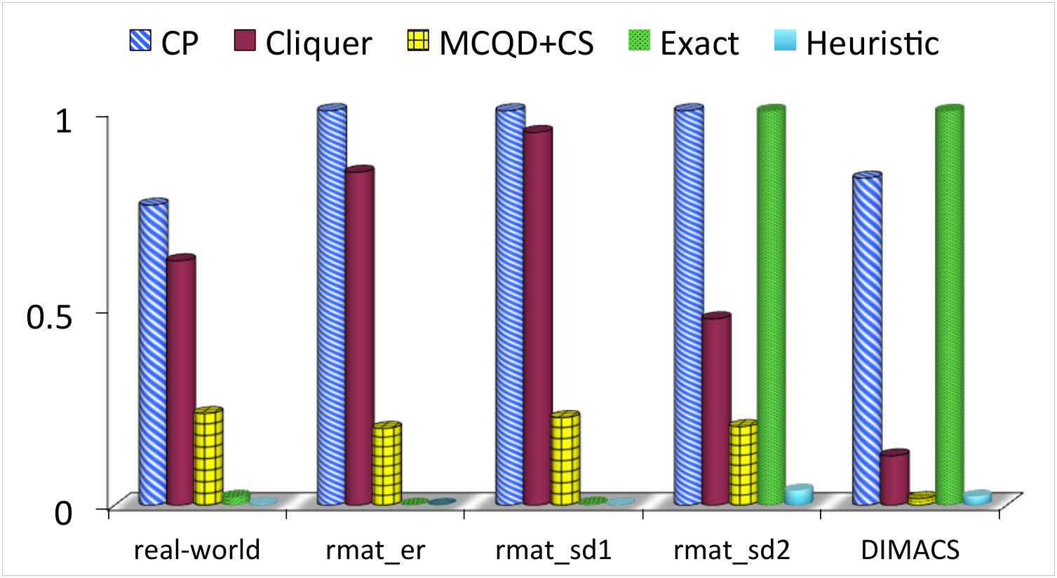
Figure 2 provides an aggregated visual summary of the runtime trends of the various algorithms across the five categories of graphs in the testbed.
To give a sense of runtime growth rates, we provide in Figure 3 plots of the runtime of the new exact algorithm and the heuristic for the synthetic and real-world graphs in the testbed. Besides the curves corresponding to the runtimes of the exact algorithm and the heuristic, the figures also include a curve corresponding to the number of edges in the graph divided by the clock frequency of the computing platform used in the experiment. This curve is added to facilitate comparison between the growth rate of the algorithms with that of a linear-time (in the size of the graph) growth rate. It can be seen that the runtime of the heuristic by and large grows somewhat linearly with the size of a graph. The exact algorithm’s runtime, which is orders of magnitude larger than the heuristic, exhibited a similar growth behavior for these test-cases (although its worst-case complexity suggests exponential growth).


4.3 Example of an application in social network analysis
We conclude this section on experiments with a small example demonstrating the application of the clique algorithms for detecting overlapping communities in social networks. In many real networks vertices may belong to more than one group, and such groups form overlapping communities. Classical examples are social networks, where an individual usually belongs to different circles at the same time, from that of work colleagues to family, sport associations, etc. Finding overlapping communities is a challenging problem [15]. Clique algorithms are one way in which a solution can be found.
For our small experiment, we use data collected from Facebook11 1 http://www.facebook.com. Every user on Facebook has a wall, which is a the user’s profile space that allows the posting of messages, often short or temporal notes by other users. The user comments and user information from specific walls are publicly available and we collected them using Facebook API. We constructed a graph with the walls as vertices. Any two users who have commented on the same wall indicate a connection between the walls, and we form an edge between them. There could be many common users for each wall, and so we assigned edge weights by Jacard index or similarity coefficient [23]. Once this is done for all walls, we retained only those edges which have weights above a chosen threshold, indicating a strong correlation. The threshold is a user’s choice and decides both the size and the number of communities found.
We modified our heuristic to retain the largest maximum clique containing each node. The exact algorithm could have also been used instead of the heuristic for this purpose. We choose the heuristic since it is much faster and for this particular problem of community detection the accuracy of the size of cliques formed is not critical.
Figure 4 shows some of the cliques/communities detected. We see two isolated communities, one for popular singers, and another for retail chains and products. We also see a community for news channels and politics, and a community of MSNBC and popular TV shows. The highlight of this experiment is that the clique algorithm allows a node to be a member of more than one community giving an overlapping community structure. Although the news channels and politics and MSNBC and tv shows communities are not directly related and have different members, they share a common member.
5 Conclusion
We presented a new exact and a new heuristic algorithm for the maximum clique problem. We performed extensive experiments on three broad categories of graphs comparing the performance of our algorithms to the algorithms due to Carraghan and Pardalos (CP) [9], Östergȧrd (cliquer) [27] and Konc and Janezic (MCQD+CS) [20]. For DIMACS benchmark graphs and certain dense synthetic graphs (rmat_sd2), our new exact algorithm performs comparably with the CP algorithm, but slower than cliquer and MCQD+CS. For large sparse graphs, both synthetic and real-world, our new algorithm runs several orders of magnitude faster than the other three. The heuristic, which runs many orders of magnitude faster than our exact algorithm and the others, gave optimal solution for 83% of the test cases, and when it is sub-optimal, its accuracy ranged between 0.83 and 0.99.
The exact algorithm was in general found to be less successful on relatively dense graphs. An interesting line of investigation would be to study ways to overcome this. Another line for future work would be to characterize the class(es) of graphs for which the heuristic is expected to return near-optimal solution.
Acknowledgements
This work is supported in part by NSF award numbers CCF-0621443, OCI-0724599, CCF-0833131, CNS-0830927, IIS-0905205, OCI-0956311, CCF-0938000, CCF-1043085, CCF-1029166, and OCI-1144061, and in part by DOE grants DE-FG02-08ER25848, DE-SC0001283, DE-SC0005309, DE-SC0005340, and DE-SC0007456. The work of Assefaw Gebremedhin is supported by the US National Science Foundation grant CCF-1218916.
References
- [1] M. Ferronato, C. Janna, G. Gambolati, Mixed constraint preconditioning in computational contact mechanics, Computer Methods in Applied Mechanics and Engineering 197 (2008), pp. 3922 – 3931.
- [2] J.G. Augustson and J. Minker, An analysis of some graph theoretical cluster techniques, J. ACM 17 (1970), pp. 571–588.
- [3] L. Babel and G. Tinhofer, A branch and bound algorithm for the maximum clique problem, Mathematical Methods of Operations Research 34 (1990), pp. 207–217.
- [4] V. Batagelj and A. Mrvar, Pajek datasets (2006), URL http://vlado.fmf.uni-lj.si/pub/networks/data/.
- [5] V. Boginski, S. Butenko, and P.M. Pardalos, Statistical analysis of financial networks, Computational Statistics & Data Analysis 48 (2005), pp. 431–443.
- [6] I.M. Bomze, M. Budinich, P.M. Pardalos, and M. Pelillo, The Maximum Clique Problem, in Handbook of Combinatorial Optimization, Kluwer Academic Publishers, 1999, pp. 1–74.
- [7] R.E. Bonner, On some clustering techniques, IBM J. Res. Dev. 8 (1964), pp. 22–32.
- [8] A.E. Brouwer, J.B. Shearer, N.J.A. Sloane, and W.D. Smith, A new table of constant weight codes., IEEE Transactions on Information Theory (1990), pp. 1334–1380.
- [9] R. Carraghan and P. Pardalos, An exact algorithm for the maximum clique problem, Oper. Res. Lett. 9 (1990), pp. 375–382.
- [10] D. Chakrabarti and C. Faloutsos, Graph mining: Laws, generators, and algorithms, ACM Comput. Surv. 38 (2006).
- [11] T.A. Davis and Y. Hu, The university of florida sparse matrix collection, ACM Transactions on Mathematical Software (TOMS) 38 (2011), pp. 1:1–1:25.
- [12] P. Domingos and M. Richardson, Mining the network value of customers, in Proc. of the 7th ACM SIGKDD KDD’01, KDD ’01, San Francisco, California, ACM, New York, NY, USA, 2001, pp. 57–66.
- [13] J. Edachery, A. Sen, F.J. Brandenburg, F.J. Br, and L.F. Informatik, Graph Clustering Using Distance-k Cliques, in Proc. of Graph Drawing, Springer-Verlag, 1999, pp. 98–106.
- [14] M. Faloutsos, P. Faloutsos, and C. Faloutsos, On power-law relationships of the Internet topology, in Proc. of the conference on Applications, technologies, architectures, and protocols for computer communication, SIGCOMM ’99, Cambridge, Massachusetts, United States, ACM, 1999, pp. 251–262.
- [15] S. Fortunato, Community detection in graphs, Physics Reports 486 (2010), pp. 75–174.
- [16] M.R. Garey and D.S. Johnson, W. H. Freeman & Co., New York, NY, USA 1979.
- [17] G. Gutin, Gross, J. L.; Yellen, J., Handbook of graph theory, Discrete Mathematics & Its Applications, CRC Press 2004.
- [18] R. Horaud and T. Skordas, Stereo correspondence through feature grouping and maximal cliques, IEEE Trans. Pattern Anal. Mach. Intell. 11 (1989), pp. 1168–1180.
- [19] D. Johnson and e. M.A. Trick, Cliques, coloring and satisfiability: Second dimacs implementation challenge, DIMACS Series on Discrete Mathematics and Theoretical Computer Science 26 (1996).
- [20] J. Konc and D. Janezic, An improved branch and bound algorithm for the maximum clique problem, proteins 4 (2007), p. 5.
- [21] R. Kumar, P. Raghavan, S. Rajagopalan, and A. Tomkins, Extracting Large-Scale Knowledge Bases from the Web., in VLDB’99, 1999, pp. 639–650.
- [22] J. Leskovec, J. Kleinberg, and C. Faloutsos, Graphs over time: densification laws, shrinking diameters and possible explanations, in Proceedings of the eleventh ACM SIGKDD international conference on Knowledge discovery in data mining, KDD ’05, Chicago, Illinois, USA, ACM, New York, NY, USA, 2005, pp. 177–187.
- [23] L. Leydesdorff, On the normalization and visualization of author co-citation data: Salton’s cosine versus the jaccard index, J. Am. Soc. Inf. Sci. Technol. 59 (2008), pp. 77–85.
- [24] T. Matsunaga, C. Yonemori, E. Tomita, and M. Muramatsu, Clique-based data mining for related genes in a biomedical database, BMC Bioinformatics 10 (2009), p. 205.
- [25] M.E.J. Newman, Coauthorship networks and patterns of scientific collaboration, Proceedings of the National Academy of Sciences of the United States of America 101 (2004), pp. 5200–5205.
- [26] S. Niskanen and P.R.J. Östergård, Cliquer user’s guide, version 1.0, Tech. Rep. T48, Communications Laboratory, Helsinki University of Technology, Espoo, Finland, 2003.
- [27] P.R.J. Östergård, A fast algorithm for the maximum clique problem, Discrete Appl. Math. 120 (2002), pp. 197–207.
- [28] G. Palla, I. Derenyi, I. Farkas, and T. Vicsek, Uncovering the overlapping community structure of complex networks in nature and society, Nature 435 (2005), pp. 814–818.
- [29] P.M. Pardalos and J. Xue, The maximum clique problem, Journal of Global Optimization 4 (1994), pp. 301–328.
- [30] M. Pavan and M. Pelillo, A new graph-theoretic approach to clustering and segmentation, in Proc. of the 2003 IEEE computer society conference on Computer vision and pattern recognition, CVPR’03, Madison, Wisconsin, IEEE Computer Society, Washington, DC, USA, 2003, pp. 145–152.
- [31] P. Prosser, Exact algorithms for maximum clique: A computational study, arXiv preprint arXiv:1207.4616v1 (2012).
- [32] S. Sadi, S. Öğüdücü, and A.S. Uyar, An efficient community detection method using parallel clique-finding ants, in Proc. of IEEE Congress on Evol. Comp, July, 2010, pp. 1–7.
- [33] P. San Segundo, D. Rodríguez-Losada, and A. Jiménez, An exact bit-parallel algorithm for the maximum clique problem, Comput. Oper. Res. 38 (2011), pp. 571–581.
- [34] E. Tomita and T. Seki, An efficient branch-and-bound algorithm for finding a maximum clique, in Proc. of the 4th international conference on Discrete mathematics and theoretical computer science, Dijon, France, Springer-Verlag, Berlin, Heidelberg, 2003, pp. 278–289.
- [35] M. Tsutomu, Y. Chikara, T. Etsuji, and M. Masaaki, Clique-based data mining for related genes in a biomedical database, BMC Bioinformatics 10 (2009).
- [36] J. Turner, Almost all k-colorable graphs are easy to color, Journal of Algorithms 9 (1988), pp. 63–82.
- [37] B. van Rietbergen, H. Weinans, R. Huiskes, and A. Odgaard, A new method to determine trabecular bone elastic properties and loading using micromechanical finite-element models, Journal of Biomechanics 28 (1995), pp. 69 – 81.
- [38] L. Wang, L. Zhou, J. Lu, and J. Yip, An order-clique-based approach for mining maximal co-locations, Information Sciences 179 (2009), pp. 3370–3382.
Appendix
| cond-mat-2003 | 25 | 29,407 | 48,096 | 6,527 | 2,600 | 17,576 |
|---|---|---|---|---|---|---|
| email-Enron | 20 | 32,462 | 155,344 | 4,060 | 110,168 | 8,835,739 |
| dictionary28 | 26 | 52,139 | 4,353 | 2,114 | 542 | 107 |
| Fault_639 | 18 | 36 | 13,987,719 | 126 | 10,767,992 | 1,116 |
| audikw_1 | 36 | 4,101 | 38,287,830 | 59,985 | 32,987,342 | 721,938 |
| bone010 | 24 | 37,887 | 34,934,616 | 361,170 | 96,622,580 | 43,991,787 |
| af_shell10 | 15 | 19 | 25,582,015 | 75 | 40,629,688 | 2,105 |
| as-Skitter | 67 | 1,656,570 | 6,880,534 | 981,810 | 26,809,527 | 737,899,486 |
| roadNet-CA | 4 | 1,487,640 | 1,079,025 | 370,206 | 320,118 | 4,302 |
| kkt_power | 11 | 1,166,311 | 4,510,661 | 401,129 | 1,067,824 | 1,978,595 |
| rmat_er_1 | 3 | 780 | 1,047,599 | 915 | 118,461 | 8,722 |
| rmat_er_2 | 3 | 2,019 | 2,094,751 | 2,351 | 235,037 | 23,908 |
| rmat_er_3 | 3 | 4,349 | 4,189,290 | 4,960 | 468,086 | 50,741 |
| rmat_er_4 | 3 | 9,032 | 8,378,261 | 10,271 | 933,750 | 106,200 |
| rmat_er_5 | 3 | 18,155 | 16,756,493 | 20,622 | 1,865,415 | 212,838 |
| rmat_sd1_1 | 6 | 39,281 | 1,004,660 | 23,898 | 151,838 | 542,245 |
| rmat_sd1_2 | 6 | 90,010 | 2,004,059 | 56,665 | 284,577 | 1,399,314 |
| rmat_sd1_3 | 6 | 176,583 | 4,013,151 | 106,543 | 483,436 | 2,677,437 |
| rmat_sd1_4 | 6 | 369,818 | 8,023,358 | 214,981 | 889,165 | 5,566,602 |
| rmat_sd1_5 | 6 | 777,052 | 16,025,729 | 455,473 | 1,679,109 | 12,168,698 |
| rmat_sd2_1 | 26 | 110,951 | 853,116 | 88,424 | 1,067,824 | 614,813,037 |
| rmat_sd2_2 | 35 | 232,352 | 1,645,086 | 195,427 | 81,886,879 | 1,044,068,886 |
| rmat_sd2_3 | 39 | 470,302 | 3,257,233 | 405,856 | 45,841,352 | 1,343,563,239 |
| rmat_sd2_4 | 43 | * | * | * | * | * |
| rmat_sd2_5 | N | * | * | * | * | * |
| hamming6-4 | 4 | 0 | 704 | 0 | 583 | 0 |
| johnson8-4-4 | 14 | 0 | 1855 | 0 | 136,007 | 0 |
| keller4 | 11 | 0 | 9435 | 0 | 8,834,190 | 0 |
| c-fat200-5 | 58 | 0 | 8473 | 0 | 70449 | 0 |
| brock200_2 | 12 | 0 | 9876 | 0 | 349,427 | 0 |
| +CS | exact | heuristic | |||||||
|---|---|---|---|---|---|---|---|---|---|
| brock200_1 | 200 | 14,834 | 21 | * | 10.37 | 0.75 | * | 18 | 0.02 |
| brock200_2 | 200 | 9,876 | 12 | 0.98 | 0.02 | 0.01 | 1.1 | 10 | 0.01 |
| brock200_3 | 200 | 12,048 | 15 | 14.09 | 0.16 | 0.03 | 14.86 | 12 | 0.01 |
| brock200_4 | 200 | 13,089 | 17 | 60.25 | 0.7 | 0.12 | 65.78 | 14 | 0.01 |
| c-fat200-1 | 200 | 1,534 | 12 | 0.01 | 0.01 | 0.01 | 0.01 | 12 | 0.01 |
| c-fat200-2 | 200 | 3,235 | 24 | 0.01 | 0.01 | 0.01 | 0.01 | 24 | 0.01 |
| c-fat200-5 | 200 | 8,473 | 58 | 0.6 | 0.33 | 0.01 | 0.93 | 58 | 0.04 |
| c-fat500-1 | 500 | 4,459 | 14 | 0.01 | 0.01 | 0.01 | 0.01 | 14 | 0.01 |
| c-fat500-2 | 500 | 9,139 | 26 | 0.02 | 0.01 | 0.01 | 0.01 | 26 | 0.01 |
| c-fat500-5 | 500 | 23,191 | 64 | 3.07 | 0.01 | 0.01 | * | 64 | 0.11 |
| hamming6-2 | 64 | 1,824 | 32 | 0.68 | 0.01 | 0.01 | 0.33 | 32 | 0.01 |
| hamming6-4 | 64 | 704 | 4 | 0.01 | 0.01 | 0.01 | 0.01 | 4 | 0.01 |
| hamming8-2 | 256 | 31,616 | 128 | * | 0.01 | 0.01 | * | 128 | 0.67 |
| hamming8-4 | 256 | 20,864 | 16 | * | 0.01 | 0.1 | * | 16 | 0.03 |
| hamming10-2 | 1,024 | 518,656 | 512 | * | 0.31 | - | * | 512 | 95.24 |
| johnson8-2-4 | 28 | 210 | 4 | 0.01 | 0.01 | 0.01 | 0.01 | 4 | 0.01 |
| johnson8-4-4 | 70 | 1,855 | 14 | 0.19 | 0.01 | 0.01 | 0.23 | 14 | 0.01 |
| johnson16-2-4 | 120 | 5,460 | 8 | 20.95 | 0.04 | 0.42 | 22.07 | 8 | 0.01 |
| keller4 | 171 | 9,435 | 11 | 22.19 | 0.15 | 0.02 | 23.35 | 11 | 0.01 |
| MANN_a9 | 45 | 918 | 16 | 1.73 | 0.01 | 0.01 | 2.5 | 16 | 0.01 |
| MANN_a27 | 378 | 70,551 | 126 | * | * | 3.3 | * | 125 | 1.74 |
| p_hat300-1 | 300 | 10,933 | 8 | 0.14 | 0.01 | 0.01 | 0.14 | 8 | 0.01 |
| p_hat300-2 | 300 | 21,928 | 25 | 831.52 | 0.32 | 0.03 | 854.59 | 24 | 0.03 |
| p_hat500-1 | 500 | 31,569 | 9 | 2.38 | 0.07 | 0.04 | 2.44 | 9 | 0.02 |
| p_hat500-2 | 500 | 62,946 | 36 | * | 159.96 | 1.2 | * | 34 | 0.14 |
| p_hat700-1 | 700 | 60,999 | 11 | 12.7 | 0.12 | 0.13 | 12.73 | 9 | 0.04 |
| p_hat1000-1 | 1,000 | 122,253 | 10 | 97.39 | 1.33 | 0.41 | 98.48 | 10 | 0.11 |
| san200_0.7_1 | 200 | 13,930 | 30 | * | 0.99 | 0.01 | * | 16 | 0.01 |