Charm Meson Mixing: An Experimental Review

Carlos A. Chavez Address: PH Department, CERN
1211 Geneva 23
Switzerland
carlos.chavez.barajas@cern.ch Ray F. Cowan Address: Lepton Quark Studies Group, Laboratory for Nuclear Science, M.I.T., 77 Massachusetts Avenue
Cambridge, Massachusetts 02139, USA
rcowan@mit.edu W.S. Lockman Address: University of California at Santa Cruz, Institute for Particle Physics
Santa Cruz, California 95064, USA
lockman@slac.stanford.edu

Abstract

We review current experimental results on charm mixing and $C\!P$ violation. We survey experimental techniques, including time-dependent, time-independent, and quantum-correlated measurements. We review techniques that use a slow pion tag from $D^{*+}\rightarrow\pi^{+}D^{0}$ + c.c. decays and those that do not, and cover two-body and multi-body $D^{0}$ decay modes. We provide a summary of $D$ -mixing results to date and comment on future experimental prospects at the LHC and other new or planned facilities.

keywords

Charm; mixing;

C\!P

violation.

PACS

PACS numbers: 13.25Ft, 11.30Er, 12.15Ff, 14.40Lb

^†^†catchline: Vol. , No. () –^†^†history: Received Day Month YearRevised Day Month Year

1 Introduction

Quantum-mechanical mixing between neutral meson particle and anti-particle flavor eigenstates provides important information about electroweak interactions and the Cabibbo-Kobayashi-Maskawa (CKM) matrix, as well as the virtual particles that are exchanged in the mixing process itself. The two parameters characterizing $D^{0}{\kern-1.60004pt\hbox{-}\kern 1.99997pt\overline{\kern-1.99997ptD}{}^{0}}$ mixing are

	$\displaystyle{x\equiv\frac{\Delta M}{\Gamma}},$		$\displaystyle\Delta M\equiv M_{1}-M_{2}$		(1)
	$\displaystyle{y\equiv\frac{\Delta\Gamma}{2\Gamma}},$		$\displaystyle\Delta\Gamma\equiv\Gamma_{1}-\Gamma_{2}$		(2)

where $M_{1,2}$ are the masses of $D_{1,2}$ , $\Gamma_{1,2}$ are the decay widths, and $\Gamma\equiv(\Gamma_{1}+\Gamma_{2})/2$ is the mean decay width.

Mixing between the states $K^{0}$ and $\kern 1.99997pt\overline{\kern-1.99997ptK}{}^{0}$ , $B^{0}$ and $\kern 1.79993pt\overline{\kern-1.79993ptB}{}^{0}$ , and $B_{s}$ and $\kern 1.79993pt\overline{\kern-1.79993ptB}{}_{s}$ is well established. Mixing in these systems is well described by standard model (SM) box diagrams containing up-type ( $u$ , $c$ , $t$ ) quarks. In contrast, the $D^{0}{\kern-1.60004pt\hbox{-}\kern 1.99997pt\overline{\kern-1.99997ptD}{}^{0}}$ SM mixing amplitude at short distances involves loops containing down-type $(d,\,s,\,b)$ quarks. The $s$ and $d$ box amplitudes[1] together are suppressed by by a factor $(m_{s}^{2}-m_{d}^{2})^{2}/(m_{W}^{2}m_{c}^{2})$ due to the Glashow-Iliopoulos-Maiani (GIM) mechanism, while the contribution from loops involving $b$ quarks is further suppressed by the Cabibbo-Kobayashi-Maskawa (CKM) factor $|V_{ub}V_{cb}^{*}|^{2}/|V_{us}V_{cs}^{*}|^{2}={\cal O}(10^{-6})$ . The contribution of the box diagrams shown in Fig. 1(a–b) to $x$ is $x^{box}\approx 5\times 10^{-6}\left[m_{s}/0.2{\mathrm{\,Ge\kern-1.00006ptV\!/}c^{2}}\right]^{4}$ .[2] The di-penguin diagram shown in Fig. 1(c) contributes at a similar level, but with opposite sign.[2]. Such diagrams contribute only to $x$ . A perturbative QCD next-to-leading order (NLO) analysis of $D^{0}{\kern-1.60004pt\hbox{-}\kern 1.99997pt\overline{\kern-1.99997ptD}{}^{0}}$ mixing[3] using an operator product expansion[4, 5, 6] to evaluate $\Delta\Gamma$ in terms of local $|\Delta C|=1$ operators, followed by a dispersion relation to evaluate $\Delta M$ ,[7] obtains: $x,y\simeq 6\times 10^{-7}$ . Taken together, the short-distance SM predictions are $x\sim{\cal O}(10^{-5})$ , $y\sim{\cal O}(10^{-7})$ , far below the current measurements, $x,y\sim{\cal O}(10^{-2})$ .

The long-distance contributions to $D^{0}{\kern-1.60004pt\hbox{-}\kern 1.99997pt\overline{\kern-1.99997ptD}{}^{0}}$ mixing are inherently nonperturbative and thus difficult to estimate. There are two approaches to estimating $D^{0}{\kern-1.60004pt\hbox{-}\kern 1.99997pt\overline{\kern-1.99997ptD}{}^{0}}$ mixing in the SM: An inclusive approach uses the Operator Product Expansion and quark-hadron duality to expand $x$ and $y$ in terms of local operators.[4, 5, 6] If the charm quark mass $m_{c}$ is large compared to the scale of strong interactions, the series can be truncated after a few terms. Such calculations typically yield $x,y\leq 10^{-3}$ . The exclusive approach sums over intermediate hadronic states to which both $D^{0}$ and $\kern 1.99997pt\overline{\kern-1.99997ptD}{}^{0}$ can decay, as shown schematically in Fig. 2. Here, non-vanishing $y$ arises from $SU(3)_{F}$ breaking in decay rates when summing over intermediate states within an $SU(3)_{F}$ multiplet. Ref. [8] found that $SU(3)_{F}$ violation in the final state phase space could provide enough $SU(3)_{F}$ breaking to generate $y\sim 10^{-2}$ . Ref. [7] used a dispersion relation to relate $x$ to $y$ and found $x$ to be in the range $(-1.0,-0.1)\times y$ .

New physics (NP) processes, some examples of which are shown in Figs. 1(d–f), could enhance the $D^{0}{\kern-1.60004pt\hbox{-}\kern 1.99997pt\overline{\kern-1.99997ptD}{}^{0}}$ mixing rate to the level of experimental detection, but the predictions for these rates also span many orders of magnitude.[9, 10, 11]. Given the uncertainties in both the SM and NP calculations, observation of $D^{0}{\kern-1.60004pt\hbox{-}\kern 1.99997pt\overline{\kern-1.99997ptD}{}^{0}}$ mixing at ${\cal O}(10^{-2)}$ does not unambiguously indicate the presence of new physics. See Refs. [9] and [10] for a summary of $D^{0}{\kern-1.60004pt\hbox{-}\kern 1.99997pt\overline{\kern-1.99997ptD}{}^{0}}$ mixing parameter predictions.

Evidence for $D^{0}{\kern-1.60004pt\hbox{-}\kern 1.99997pt\overline{\kern-1.99997ptD}{}^{0}}$ mixing was reported in 2007 using high-luminosity data sets acquired at the $B$ factories[12, 13] and Tevatron collider.[14] While the significance of the current world average for $D^{0}{\kern-1.60004pt\hbox{-}\kern 1.99997pt\overline{\kern-1.99997ptD}{}^{0}}$ mixing is greater than ten standard deviations ( $10\sigma$ ),[15] to date no one single $D^{0}{\kern-1.60004pt\hbox{-}\kern 1.99997pt\overline{\kern-1.99997ptD}{}^{0}}$ mixing measurement exceeds $5\sigma$ , the commonly accepted criterion for observation.

Refer to caption — Figure 1: Possible short-distance amplitudes contributing to $D^{0}{\kern-1.60004pt\hbox{-}\kern 1.99997pt\overline{\kern-1.99997ptD}{}^{0}}$ mixing. (a–b) SM boxes; (c) SM di-penguin; (d): new physics flavor-changing neutral current process mediated by a heavy $Z^{\prime 0}$ ; (e–f): charged Higgs in the mixing loop.

1.1 $D^{0}{\kern-1.60004pt\hbox{-}\kern 1.99997pt\overline{\kern-1.99997ptD}{}^{0}}$ Mixing Formalism

The $D^{0}$ and $\kern 1.99997pt\overline{\kern-1.99997ptD}{}^{0}$ mesons are produced as flavor eigenstate with charm quantum numbers $C=+1$ and $-1$ , respectively. They propagate and decay according to the Schrödinger equation:

i\frac{\partial}{\partial t}\left(\begin{array}[]{c}D^{0}(t)\\ \kern 1.99997pt\overline{\kern-1.99997ptD}{}^{0}(t)\end{array}\right)=\left({\bf M}-\frac{i}{2}{\bf\Gamma}\right)\left(\begin{array}[]{c}D^{0}(t)\\ \kern 1.99997pt\overline{\kern-1.99997ptD}{}^{0}(t)\end{array}\right).

(3)

Mixing between $D^{0}$ and $\kern 1.99997pt\overline{\kern-1.99997ptD}{}^{0}$ occurs because these flavor states are not the eigenstates $D_{1}$ and $D_{2}$ of the $D^{0}{\kern-1.60004pt\hbox{-}\kern 1.99997pt\overline{\kern-1.99997ptD}{}^{0}}$ mass matrix ${\bf M}-i{\bf\Gamma}/2$ , but linear combinations of them. Assuming that the product of charge conjugation, parity and time reversal (CPT) is conserved,[17] the eigenstates of Eq. 3, $|D_{1,2}\rangle$ are given by:[17, 18]

\displaystyle\begin{array}[]{rcc}|D_{1}\rangle&=&\ p|D^{0}\rangle+q|\kern 1.99997pt\overline{\kern-1.99997ptD}{}^{0}\rangle,\\ |D_{2}\rangle&=&\ p|D^{0}\rangle-q|\kern 1.99997pt\overline{\kern-1.99997ptD}{}^{0}\rangle,\end{array}

and inversely

\displaystyle\begin{array}[]{rcc}|D^{0}\rangle&=&\ \frac{1}{2p}\left(|D_{1}\rangle+|D_{2}\rangle\right),\\ |\kern 1.99997pt\overline{\kern-1.99997ptD}{}^{0}\rangle&=&\ \frac{1}{2q}\left(|D_{1}\rangle-|D_{2}\rangle\right),\end{array}

where the complex quantities $p$ and $q$ satisfy

\left(\frac{q}{p}\right)^{2}=\frac{M^{*}_{12}-\frac{i}{2}\Gamma^{*}_{12}}{M_{12}-\frac{i}{2}\Gamma_{12}},\quad\left|p\right|^{2}+\left|q\right|^{2}=1,

(10)

where $M_{12}$ and $\Gamma_{12}$ are the complex off-diagonal elements of the $2\times 2$ matrices ${\bf M}$ and ${\bf\Gamma}$ , respectively. In the limit of $C\!P$ conservation, $D_{1}$ is $C\!P$ -even and $D_{2}$ is $C\!P$ -odd.¹¹ 1 We use the $C\!P$ phase convention: $C\!P|{D^{0}}\rangle=+|{\kern 1.99997pt\overline{\kern-1.99997ptD}{}^{0}}\rangle$ and $C\!P|{\kern 1.99997pt\overline{\kern-1.99997ptD}{}^{0}}\rangle=+|{D^{0}}\rangle$ . The eigenvalues of Eq. 3 are:

\gamma_{1,2}\equiv M_{1,2}-\frac{i}{2}\Gamma_{1,2}=M_{11}-\frac{i}{2}\Gamma_{11}\pm\frac{q}{p}\left(M_{12}-\frac{i}{2}\Gamma_{12}\right)

(11)

The eigenstates of Eq. 3 develop in time as follows:[17, 18]

|D_{1,2}(t)\rangle=e_{1,2}(t)|D_{1,2}(0)\rangle,\qquad e_{1,2}(t)\equiv\exp\left[-i\left(M_{1,2}-\frac{i}{2}\Gamma_{1,2}\right)t\right],

(12)

Using Eq. 1.1, Eq. 1.1 and Eq. 12, the proper time evolution of a state which is initially a pure $D^{0}$ ( $\kern 1.99997pt\overline{\kern-1.99997ptD}{}^{0}$ ) is given by:

	$\displaystyle\|{D^{0}(t)}\rangle$	$\displaystyle=$	$\displaystyle g_{+}(t)\|{D^{0}}\rangle+\frac{q}{p}g_{-}(t)\|{\kern 1.99997pt\overline{\kern-1.99997ptD}{}^{0}}\rangle,$		(13)
	$\displaystyle\|{\kern 1.99997pt\overline{\kern-1.99997ptD}{}^{0}(t)}\rangle$	$\displaystyle=$	$\displaystyle g_{+}(t)\|{\kern 1.99997pt\overline{\kern-1.99997ptD}{}^{0}}\rangle+\frac{p}{q}g_{-}(t)\|{D^{0}}\rangle.$		(14)

where:

g_{\pm}(t)=\left[e_{1}(t)\pm e_{2}(t)\right]/2.

(15)

The probabilities for obtaining a $D^{0}$ or $\kern 1.99997pt\overline{\kern-1.99997ptD}{}^{0}$ at proper time $t$ , starting from an initially pure $D^{0}$ or $\kern 1.99997pt\overline{\kern-1.99997ptD}{}^{0}$ are:

$\displaystyle\|\langle D^{0}\|D^{0}(t)\rangle\|^{2}$	$\displaystyle=$	$\displaystyle\|\langle\kern 1.99997pt\overline{\kern-1.99997ptD}{}^{0}\|\kern 1.99997pt\overline{\kern-1.99997ptD}{}^{0}(t)\rangle\|^{2}$	(16)
	$\displaystyle=$	$\displaystyle\left\|g_{+}(t)\right\|^{2}=\frac{1}{2}e^{-\Gamma t}\left[\cosh(y\Gamma t)+\cos(x\Gamma t)\right],$	(16)
$\displaystyle\|\langle\kern 1.99997pt\overline{\kern-1.99997ptD}{}^{0}\|D^{0}(t)\rangle\|^{2}$	$\displaystyle=$	$\displaystyle\left\|\frac{q}{p}\right\|^{2}\|g_{-}(t)\|^{2}=\frac{1}{2}\left\|\frac{q}{p}\right\|^{2}e^{-\Gamma t}\left[\cosh(y\Gamma t)-\cos(x\Gamma t)\right],$	(17)
$\displaystyle\|\langle D^{0}\|\kern 1.99997pt\overline{\kern-1.99997ptD}{}^{0}(t)\rangle\|^{2}$	$\displaystyle=$	$\displaystyle\left\|\frac{p}{q}\right\|^{2}\|g_{-}(t)\|^{2}=\frac{1}{2}\left\|\frac{p}{q}\right\|^{2}e^{-\Gamma t}\left[\cosh(y\Gamma t)-\cos(x\Gamma t)\right],$	(18)

If both $x$ and $y$ are zero, then the probability for a $D^{0}$ to mix to a $\kern 1.99997pt\overline{\kern-1.99997ptD}{}^{0}$ or for a $\kern 1.99997pt\overline{\kern-1.99997ptD}{}^{0}$ to mix to a $D^{0}$ will be identically zero for all proper times. If either $x$ or $y$ is non-zero, then $D^{0}{\kern-1.60004pt\hbox{-}\kern 1.99997pt\overline{\kern-1.99997ptD}{}^{0}}$ mixing will occur.

$M_{12}$ and $\Gamma_{12}$ determine the mass and width splittings $\Delta M$ and $\Delta\Gamma$ , respectively:

	$\displaystyle\Delta M$	$\displaystyle\equiv$	$\displaystyle M_{1}-M_{2}=2{\rm Re}\left[\frac{q}{p}(M_{12}-\frac{i}{2}\Gamma_{12})\right]$		(19)
	$\displaystyle\Delta\Gamma$	$\displaystyle\equiv$	$\displaystyle\Gamma_{1}-\Gamma_{2}=-4{\rm Im}\left[\frac{q}{p}(M_{12}-\frac{i}{2}\Gamma_{12})\right],$		(20)

and therefore the characteristics of $D^{0}{\kern-1.60004pt\hbox{-}\kern 1.99997pt\overline{\kern-1.99997ptD}{}^{0}}$ mixing. We show the unmixed and mixed intensities as a function of the dimensionless variable, $\Gamma t$ , for initially pure states of $K^{0}$ , $D^{0}$ , $B^{0}$ and $B_{s}$ , in Figs. 3(a–d), respectively. Of the four lowest-lying neutral pseudoscalar meson systems, the $D^{0}{\kern-1.60004pt\hbox{-}\kern 1.99997pt\overline{\kern-1.99997ptD}{}^{0}}$ system shows the smallest mixing, as noted earlier. In the $K^{0}$ system, both $\left|x\right|$ and $\left|y\right|$ are both of order 1; in the $D^{0}$ system, $\left|x\right|$ and $\left|y\right|$ are both of order 1%; in the $B^{0}$ and $B_{s}$ systems, $\left|x\right|\gg\left|y\right|$ .

From Eq. 13 (Eq. 14), the amplitude that a $D^{0}$ ( $\kern 1.99997pt\overline{\kern-1.99997ptD}{}^{0}$ ) produced at $t=0$ will develop into a linear combination of $D^{0}$ and $\kern 1.99997pt\overline{\kern-1.99997ptD}{}^{0}$ and decay into $f$ ( $\bar{f}$ ) at time $t$ is:

	$\displaystyle\langle{f}\|{{\cal H}}\|{D^{0}(t)}\rangle$	$\displaystyle=$	$\displaystyle A_{f}g_{+}(t)+\bar{A}_{f}\frac{q}{p}g_{-}(t),$		(21)
	$\displaystyle\langle{\bar{f}}\|{{\cal H}}\|{\kern 1.99997pt\overline{\kern-1.99997ptD}{}^{0}(t)}\rangle$	$\displaystyle=$	$\displaystyle\bar{A}_{\bar{f}}g_{+}(t)+A_{\bar{f}}\frac{p}{q}g_{-}(t),$		(22)

where $A_{f}$ and $\bar{A}_{f}$ are the $D^{0}$ and $\kern 1.99997pt\overline{\kern-1.99997ptD}{}^{0}$ decay amplitudes to a final state $f$ ; $A_{\bar{f}}$ and $\bar{A}_{\bar{f}}$ are the $D^{0}$ and $\kern 1.99997pt\overline{\kern-1.99997ptD}{}^{0}$ decay amplitudes to a final state $\bar{f}$ :

$\displaystyle A_{f}$	$\displaystyle\equiv$	$\displaystyle\langle{f}\|{{\cal H}}\|{D^{0}}\rangle,$	(23)
$\displaystyle\bar{A}_{f}$	$\displaystyle\equiv$	$\displaystyle\langle{f}\|{{\cal H}}\|{\kern 1.99997pt\overline{\kern-1.99997ptD}{}^{0}}\rangle,$	(24)
$\displaystyle A_{\bar{f}}$	$\displaystyle\equiv$	$\displaystyle\langle{\bar{f}}\|{{\cal H}}\|{D^{0}}\rangle,$	(25)
$\displaystyle\bar{A}_{\bar{f}}$	$\displaystyle\equiv$	$\displaystyle\langle{\bar{f}}\|{{\cal H}}\|{\kern 1.99997pt\overline{\kern-1.99997ptD}{}^{0}}\rangle.$	(26)

where ${\cal H}$ is the Hamiltonian governing weak decays. Written in terms of the decay amplitudes, the general expressions for the time-dependent decay rates $\Gamma(D^{0}(t)\rightarrow f)$ and $\Gamma(\kern 1.99997pt\overline{\kern-1.99997ptD}{}^{0}(t)\rightarrow\bar{f})$ are:

$\displaystyle\Gamma(D^{0}(t)\rightarrow f)=$		(27)
	$\displaystyle\frac{e^{-\Gamma t}}{2}\left[\|A_{f}\|^{2}[\cosh(y\Gamma t)+\cos(x\Gamma t)]+\left\|\frac{q}{p}\right\|^{2}\|\bar{A}_{f}\|^{2}[\cosh(y\Gamma t)-\cos(x\Gamma t)]\right.$
	$\displaystyle\qquad\left.-2{\rm Re}\left(A^{}_{f}\bar{A}_{f}\frac{q}{p}\right)\sinh(y\Gamma t)+2{\rm Im}\left(A^{}_{f}\bar{A}_{f}\frac{q}{p}\right)\sin(x\Gamma t)\right],$
$\displaystyle\Gamma(\kern 1.99997pt\overline{\kern-1.99997ptD}{}^{0}(t)\rightarrow\bar{f})=$		(28)
	$\displaystyle\frac{e^{-\Gamma t}}{2}\left[\|\bar{A}_{\bar{f}}\|^{2}[\cosh(y\Gamma t)+\cos(x\Gamma t)]+\left\|\frac{p}{q}\right\|^{2}\|A_{\bar{f}}\|^{2}[\cosh(y\Gamma t)-\cos(x\Gamma t)]\right.$
	$\displaystyle\qquad\left.-2{\rm Re}\left({\bar{A}}^{}_{\bar{f}}A_{\bar{f}}\frac{p}{q}\right)\sinh(y\Gamma t)+2{\rm Im}\left({\bar{A}}^{}_{\bar{f}}A_{\bar{f}}\frac{p}{q}\right)\sin(x\Gamma t)\right].$

To describe the time dependence for the “wrong-sign” (WS) decay such as $D^{0}\rightarrow K^{+}\pi^{-}$ ( $\kern 1.99997pt\overline{\kern-1.99997ptD}{}^{0}\rightarrow K^{-}\pi^{+}$ ), we rewrite Eq. 27 (Eq. 28) in terms of of the Cabibbo-favored (CF) amplitude $\bar{A}_{f}$ ( $A_{\bar{f}}$ ) and the parameter $\lambda_{f}^{-1}$ ( $\lambda_{\bar{f}}$ ), where

\lambda_{f}\equiv\frac{q}{p}\frac{\bar{A}_{f}}{A_{f}}.

(29)

For decay times $t$ satisfying $|x\Gamma t|,|y\Gamma t|\ll 1$ , the decay rates are given by:

$\displaystyle\Gamma(D^{0}(t)\rightarrow f)=$		(30)
	$\displaystyle e^{-\Gamma t}\left\|\bar{A}_{f}\right\|^{2}\left\|\frac{q}{p}\right\|^{2}\left[\left\|\lambda_{f}^{-1}\right\|^{2}-{\rm Re}\left(\lambda_{f}^{-1}\right)y\Gamma t-{\rm Im}\left(\lambda_{f}^{-1}\right)x\Gamma t+\frac{x^{2}+y^{2}}{4}(\Gamma t)^{2}\right],\qquad$	(30)
$\displaystyle\Gamma(\kern 1.99997pt\overline{\kern-1.99997ptD}{}^{0}(t)\rightarrow\bar{f})=$		(31)
	$\displaystyle e^{-\Gamma t}\left\|A_{\bar{f}}\right\|^{2}\left\|\frac{p}{q}\right\|^{2}\left[\left\|\lambda_{\bar{f}}\right\|^{2}-{\rm Re}\left(\lambda_{\bar{f}}\right)y\Gamma t-{\rm Im}\left(\lambda_{\bar{f}}\right)x\Gamma t+\frac{x^{2}+y^{2}}{4}(\Gamma t)^{2}\right].\qquad\qquad$	(31)

Under similar conditions, the time-dependent rates for $D^{0}$ and $\kern 1.99997pt\overline{\kern-1.99997ptD}{}^{0}$ decaying to a $C\!P$ -eigenstate $f=\bar{f}=f_{C\!P}$ can be written as:

$\displaystyle\Gamma(D^{0}(t)\rightarrow f_{C\!P})=$		(32)
	$\displaystyle e^{-\Gamma t}\left\|A_{f_{C\!P}}\right\|^{2}\left[1-{\rm Re}\left(\lambda_{f_{C\!P}}\right)y\Gamma t+{\rm Im}\left(\lambda_{f_{C\!P}}\right)x\Gamma t+\left\|\lambda_{f_{C\!P}}\right\|^{2}\frac{x^{2}+y^{2}}{4}(\Gamma t)^{2}\right],\qquad$	(32)
$\displaystyle\Gamma(\kern 1.99997pt\overline{\kern-1.99997ptD}{}^{0}(t)\rightarrow f_{C\!P})=$		(33)
	$\displaystyle e^{-\Gamma t}\left\|{\bar{A}}_{f_{C\!P}}\right\|^{2}\left[1-{\rm Re}\left(\lambda^{-1}_{f_{C\!P}}\right)y\Gamma t+{\rm Im}\left(\lambda^{-1}_{f_{C\!P}}\right)x\Gamma t+\left\|\lambda^{-1}_{f_{C\!P}}\right\|^{2}\frac{x^{2}+y^{2}}{4}(\Gamma t)^{2}\right],\qquad$	(33)

where the terms proportional to $e^{-\Gamma t}(\Gamma t)^{2}$ are due to mixing, those proportional to $e^{-\Gamma t}\Gamma t$ are due to the interference between mixing and decay, while those proportional to $e^{-\Gamma t}$ are due to direct decay. Fig. 4 illustrates the two interfering decay paths from an initial $D^{0}$ to to a final state $f$ .

1.2 $C\!P$ violation

There are three different types of $C\!P$ -violating effects in meson decays:²² 2 For a complete review, see Refs. [17, 20, 21].

1.

$C\!P$ violation ( $CPV$ ) in mixing;
2.

$CPV$ in decay, also known as direct $CPV$ ;
3.

$CPV$ in the interference between a direct decay, $D^{0}\rightarrow f$ , and a decay involving mixing, $D^{0}\rightarrow\kern 1.99997pt\overline{\kern-1.99997ptD}{}^{0}\rightarrow f$ .

$CPV$ in mixing and in the interference between mixing and decay is referred to as indirect $CPV$ .

$CPV$ in mixing occurs when the mixing probability of $D^{0}$ to $\kern 1.99997pt\overline{\kern-1.99997ptD}{}^{0}$ is different than the mixing probability of $\kern 1.99997pt\overline{\kern-1.99997ptD}{}^{0}$ to $D^{0}$ . As can be seen from Eqs. 17 and 18, this happens if and only if $\left|q/p\right|\neq 1$ . This type of $CP$ -violating effect depends only on the mixing parameters and not the final state of the decay.

As an example, consider the decay $D^{0}\rightarrow K^{(*)+}l^{-}{\bar{\nu}}_{l}$ . The diagram for this decay is illustrated in Fig. 5. Within the SM, the $D^{0}$ must first mix to $\kern 1.99997pt\overline{\kern-1.99997ptD}{}^{0}$ , followed by the direct decay $\kern 1.99997pt\overline{\kern-1.99997ptD}{}^{0}\rightarrow K^{(*)+}l^{-}{\bar{\nu}}_{l}$ . There is no direct decay of $D^{0}$ to the final state $K^{(*)+}l^{-}{\bar{\nu}}_{l}$ in the SM. Therefore, the time-dependent $C\!P$ asymmetry:

\displaystyle{\cal A}_{SL}

\displaystyle=

\displaystyle\frac{d\Gamma/dt(D^{0}\rightarrow K^{(*)+}l^{-}{\bar{\nu}}_{l})-d\Gamma/dt(\kern 1.99997pt\overline{\kern-1.99997ptD}{}^{0}\rightarrow K^{(*)-}l^{+}{\nu}_{l})}{d\Gamma/dt(D^{0}\rightarrow K^{(*)+}l^{-}{\bar{\nu}}_{l})+d\Gamma/dt(\kern 1.99997pt\overline{\kern-1.99997ptD}{}^{0}\rightarrow K^{(*)-}l^{+}{\nu}_{l})}

(34)

is equal to the mode-independent quantity:

\displaystyle{A_{M}}

\displaystyle=

\displaystyle\frac{|q/p|^{2}-|p/q|^{2}}{|q/p|^{2}+|p/q|^{2}}

(35)

which is used to characterize $CPV$ in mixing. The techniques used to analyze the decay $D^{0}\rightarrow K^{(*)+}l^{-}{\bar{\nu}}_{l}$ for $D^{0}{\kern-1.60004pt\hbox{-}\kern 1.99997pt\overline{\kern-1.99997ptD}{}^{0}}$ mixing are discussed in Sec. 2.3.4; the results are presented in Sec. 3.3.4.

$CPV$ in decay occurs when the amplitude for a decay and its $CP$ conjugate process have different magnitudes: $\left|\bar{A}_{\bar{f}}/A_{f}\right|\neq 1$ . In charged $D$ modes where no mixing can occur, $CPV$ in decay is characterized by non-zero values for the time-integrated asymmetry:

{\cal A}_{f^{\pm}}\equiv\frac{\Gamma(D^{-}\rightarrow f^{-})-\Gamma(D^{+}\rightarrow f^{+})}{\Gamma(D^{-}\rightarrow f^{-})+\Gamma(D^{+}\rightarrow f^{+})}=\frac{\left|\bar{A}_{f^{-}}/A_{f^{+}}\right|^{2}-1}{\left|\bar{A}_{f^{-}}/A_{f^{+}}\right|^{2}+1}

(36)

Consider the case where two amplitudes:

\begin{array}[]{rcl}A_{f}&=&|a_{1}|e^{i(\delta_{1}+\phi_{1})}+|a_{2}|e^{i(\delta_{2}+\phi_{2})}\\ \bar{A}_{\bar{f}}&=&|a_{1}|e^{i(\delta_{1}-\phi_{1})}+|a_{2}|e^{i(\delta_{2}-\phi_{2})}\end{array}

(37)

mediate the decay, where $\delta_{1,2}$ and $\phi_{1,2}$ are the strong and weak phases, respectively, of amplitude $A_{1,2}$ . The weak phase changes sign under $C\!P$ , whereas the strong phase does not. The $C\!P$ asymmetry ${\cal A}_{f^{\pm}}$ can then be written as:

{\cal A}_{f^{\pm}}=-\frac{2|a_{1}||a_{2}|\sin(\delta_{2}-\delta_{1})\sin(\phi_{2}-\phi_{1})}{|a_{1}|^{2}+|a_{2}|^{2}+2|a_{1}||a_{2}|\cos(\delta_{2}-\delta_{1})\cos(\phi_{2}-\phi_{1})}.

(38)

Thus, direct $CPV$ will occur ( ${\cal A}_{f^{\pm}}\neq 0$ ) only if the differences between the $C\!P$ -conserving strong phases and the differences between the $C\!P$ -violating weak phases of the two contributing amplitudes are not zero or multiples of $\pi$ . In neutral $D$ decays, direct $CPV$ is characterized by the mode-dependent parameter $A_{D}$ :[19]

\displaystyle A_{D}

\displaystyle\equiv

\displaystyle\frac{\left|A_{f}/\bar{A}_{f}\right|^{2}-\left|\bar{A}_{\bar{f}}/A_{\bar{f}}\right|^{2}}{\left|A_{f}/\bar{A}_{f}\right|^{2}+\left|\bar{A}_{\bar{f}}/A_{\bar{f}}\right|^{2}}.

(39)

$CPV$ in the interference between a decay without mixing, $D^{0}\rightarrow f$ , and a decay with mixing, $D^{0}\rightarrow\kern 1.99997pt\overline{\kern-1.99997ptD}{}^{0}\rightarrow f$ , where $f$ can be reached from both $D^{0}$ and $\kern 1.99997pt\overline{\kern-1.99997ptD}{}^{0}$ decays, can also occur. Consider the time-dependent rate asymmetry of neutral meson decays to a final $C\!P$ eigenstate:

{A}_{CP}(t)=\frac{\Gamma(D^{0}(t)\rightarrow f_{C\!P})-\Gamma(\kern 1.99997pt\overline{\kern-1.99997ptD}{}^{0}(t)\rightarrow f_{C\!P})}{\Gamma(D^{0}(t)\rightarrow f_{C\!P})+\Gamma(\kern 1.99997pt\overline{\kern-1.99997ptD}{}^{0}(t)\rightarrow f_{C\!P})}

(40)

If both $CPV$ in mixing and decay are absent, then $|q/p|=1$ , $|{\bar{A}}_{f_{C\!P}}/A_{f_{C\!P}}|=1$ and therefore, $|\lambda_{f_{C\!P}}|=1$ . As can be seen by comparing Eqs. 32 and 33, ${A}_{CP}(t)$ will be nonzero when ${\lambda^{-1}_{f_{C\!P}}}\neq\lambda_{f_{C\!P}}$ , Therefore, $CPV$ in the interference between mixing and decay will be present if ${\rm Im}\lambda_{f_{C\!P}}\neq 0$ , which implies $\sin\phi_{f_{C\!P}}\neq 0$ , where $\lambda_{f_{C\!P}}\equiv|\lambda_{f_{C\!P}}|\exp({i\phi_{f_{C\!P}}})$ . The phase $\phi_{f_{C\!P}}$ is the sum of the phase difference between $q$ and $p$ ,

\varphi\equiv\arg\left(q/p\right)

(41)

and the (weak) phase difference between $\bar{A}_{f}$ and $A_{f}$ . In general, the weak phase component of $\arg(\lambda_{f})$ is said to characterize $CPV$ in the interference between mixing and decay.

The quantities $\lambda_{f}^{-1}$ and $\lambda_{\bar{f}}$ can be evaluated for the modes $f=K^{+}\pi^{-}$ and $f=K^{+}K^{-}$ in terms of $A_{M}$ and the mode-dependent quantities $R_{D}$ , $A_{D}$ , $A_{D}^{KK}$ , $\phi_{K\pi}$ and $\phi_{KK}$ :[19]

$\displaystyle\lambda^{-1}_{K^{+}\pi^{-}}$	$\displaystyle=$	$\displaystyle-\sqrt{R_{D}}\sqrt[4]{\frac{(1+A_{D})(1-A_{M})}{(1-A_{D})(1+A_{M})}}e^{-i({\delta_{K\pi}}+\phi_{K\pi})},$	(42)
$\displaystyle\lambda_{K^{-}\pi^{+}}$	$\displaystyle=$	$\displaystyle-\sqrt{R_{D}}\sqrt[4]{\frac{(1-A_{D})(1+A_{M})}{(1+A_{D})(1-A_{M})}}e^{-i({\delta_{K\pi}}-\phi_{K\pi})},$	(43)
$\displaystyle\lambda_{K^{+}K^{-}}$	$\displaystyle=$	$\displaystyle\sqrt[4]{\frac{(1-A_{D}^{KK})(1+A_{M})}{(1+A_{D}^{KK})(1-A_{M})}}e^{i\phi_{KK}}.$	(44)

For $f=K^{+}\pi^{-}$ the quantity $R_{D}$ is defined to be

\begin{array}[]{ccc}R_{D}\equiv\sqrt{R_{D}^{+}R_{D}^{-}},&R_{D}^{+}\equiv|A_{K^{+}\pi^{-}}/{\bar{A}}_{K^{+}\pi^{-}}|^{2},&R_{D}^{-}\equiv|{\bar{A}}_{K^{-}\pi^{+}}/A_{K^{-}\pi^{+}}|^{2}.\end{array}

(45)

In the absence of direct $CPV$ ,

\begin{array}[]{cc}R_{D}^{+}=|A_{K^{+}\pi^{-}}/A_{K^{-}\pi^{+}}|^{2},&R_{D}^{-}\equiv|{\bar{A}}_{K^{-}\pi^{+}}/{\bar{A}}_{K^{+}\pi^{-}}|^{2},\end{array}

(46)

are the ratios of the doubly-Cabibbo-suppressed (DCS) to Cabibbo-favored (CF) decay widths for $D^{0}$ and $\kern 1.99997pt\overline{\kern-1.99997ptD}{}^{0}$ decays, respectively. These ratios are ${\cal O}(\tan^{4}(\theta_{c}))\approx 0.3\%$ , where $\theta_{c}$ is the Cabibbo angle. Additionally, ${\delta_{K\pi}}$ is the relative strong phase between $A_{K^{+}\pi^{-}}$ and ${\bar{A}}_{K^{+}\pi^{-}}$ . The quantities $A_{D}$ and $\phi$ are in general mode-dependent. However, assuming that SM tree-level amplitudes dominate the decays, $\phi$ appearing in Eqs. 42, 43 and 44 will be the same for the $K\pi$ and $KK$ modes.[21, 22]

Traditional SM estimates for $C\!P$ asymmetries in $D$ -meson decays are small, less than ${\cal O}(0.01\%)$ .[23, 24, 25] This is because, to a very good approximation, only two generations of quarks are involved in charm mixing and decay, while the CKM mechanism[26] requires three quark generations to produce $CPV$ .[27] Present experimental uncertainties on time-integrated $C\!P$ asymmetries in $D$ decays are ${\cal O}(0.1\%)$ .[15] Through 2010, all measured $C\!P$ asymmetries in $D$ decays were consistent with zero within experimental errors.[15, 19]

In 2011, the LHCb Collaboration presented evidence for direct $CPV$ by measuring the difference in time-integrated $C\!P$ asymmetries between two singly Cabibbo suppressed $D$ decay modes: $\Delta{A}_{CP}\equiv{A}_{CP}(D\rightarrow K^{+}K^{-})-{A}_{CP}(D\rightarrow\pi^{+}\pi^{-})=(-0.82\pm 0.21({\rm stat})\pm 0.11({\rm syst}))\%$ .[28] In this difference, the mode-independent indirect contribution cancels. A new standard model calculation[29] of this difference, while uncertain to a factor of a few, may accommodate this intriguingly large experimental result. New physics, such as supersymmetric gluino-squark loops, could also yield direct $C\!P$ asymmetries as large as ${\cal O}(1\%)$ .[30]

1.3 Outline

This paper discusses the experimental status of $D^{0}{\kern-1.60004pt\hbox{-}\kern 1.99997pt\overline{\kern-1.99997ptD}{}^{0}}$ mixing and $CPV$ as of the end of the 2011 calendar year. We review the current results from recent colliding-beam and fixed-target experiments and discuss in some detail the techniques involved. We survey the primary analysis methods used to study two-body and multi-body hadronic and semileptonic $D^{0}$ decays. Then we present results from experimental measurements of mixing and searches for $CPV$ from time-independent analyses (those that do not use the proper decay time of the $D^{0}$ to search for mixing) and time-dependent analyses (which do use the proper $D^{0}$ decay time) as well as quantum-correlated decays. Finally we review future prospects for measurements in the near- and longer-term future and summarize the overall status of $D^{0}$ - $\kern 1.99997pt\overline{\kern-1.99997ptD}{}^{0}$ mixing experiments.

2 Analysis Techniques for Measuring Charm Mixing and CP Violation

2.1 Time-independent Methods

Time-independent methods provide an important technique for measuring $D^{0}$ - $\kern 1.99997pt\overline{\kern-1.99997ptD}{}^{0}$ mixing and searching for $C\!P$ violation in charm decays. They also yield information on relative strong phases between mixed and direct decays for several different hadronic modes of interest to mixing studies. Knowledge of the strong phase ${\delta_{K\pi}}$ between $D^{0}$ $\rightarrow$ $K^{+}$ $\pi^{-}$ and $\kern 1.99997pt\overline{\kern-1.99997ptD}{}^{0}$ $\rightarrow$ $K^{+}$ $\pi^{-}$ allows conversion of the observable $y^{\prime}$ to mixing parameter $y$ (see Sec. 2.2.1).

As the name implies, these methods do not make use of decay-time information. Instead, they count the numbers of $D^{0}$ and $\kern 1.99997pt\overline{\kern-1.99997ptD}{}^{0}$ decays to specific modes when the $D^{0}{\kern-1.60004pt\hbox{-}\kern 1.99997pt\overline{\kern-1.99997ptD}{}^{0}}$ pair has been produced in a quantum-coherent, charge conjugation ( $C$ ) eigenstate. Relative numbers of decay modes of both singly-tagged (ST) events, where one $D^{0}$ or $\kern 1.99997pt\overline{\kern-1.99997ptD}{}^{0}$ is fully reconstructed, and doubly-tagged (DT) events, where both the $D^{0}$ and the $\kern 1.99997pt\overline{\kern-1.99997ptD}{}^{0}$ mesons are fully reconstructed, provide information on the mixing parameters $x$ and $y$ , the strong phase differences $\delta_{i}$ for each decay mode $i$ , and their DCS decay rates. This method is especially useful when separating the individual $D^{0}$ and $\kern 1.99997pt\overline{\kern-1.99997ptD}{}^{0}$ decay vertices is difficult, as in the case of non-asymmetric energy $e^{+}e^{-}$ colliders.

At present, these methods have been performed[31, 32] only at the 3.770 $\mathrm{\,Ge\kern-1.00006ptV}$ resonance, but could also be done at higher center-of-mass energies through initial-state radiation, if the number of ISR photons can be determined (so that the $C\!P$ state of the coherent $D^{0}{\kern-1.60004pt\hbox{-}\kern 1.99997pt\overline{\kern-1.99997ptD}{}^{0}}$ pair is known).

2.1.1 Correlated Decays at 3.770 $\mathrm{\,Ge\kern-1.00006ptV}$

In $e^{+}e^{-}$ collisions at or above 3.770 $\mathrm{\,Ge\kern-1.00006ptV}$ that produce a $D^{0}{\kern-1.60004pt\hbox{-}\kern 1.99997pt\overline{\kern-1.99997ptD}{}^{0}}$ pair, the production of the pair may be assumed to proceed through a single virtual photon with $J^{PC}=1^{--}$ . At 3.770 $\mathrm{\,Ge\kern-1.00006ptV}$ , the final state will have $C=-1$ . At higher energies, additional pions and photons may be produced:[33]

e^{+}e^{-}\rightarrow D^{0}\kern 1.99997pt\overline{\kern-1.99997ptD}{}^{0}+m(\pi^{0})+n(\gamma)

(47)

where $m$ , $n\geq 0$ . Therefore the $D^{0}$ - $\kern 1.99997pt\overline{\kern-1.99997ptD}{}^{0}$ pair will be produced with $C(D^{0}\kern 1.99997pt\overline{\kern-1.99997ptD}{}^{0})=-1^{n+1}$ . When $n=0$ , $C(D^{0}\kern 1.99997pt\overline{\kern-1.99997ptD}{}^{0})$ will be $-1$ . The value of $m$ is not a factor since $C(\pi^{0})=+1$ .

Additionally, if the $D^{0}{\kern-1.60004pt\hbox{-}\kern 1.99997pt\overline{\kern-1.99997ptD}{}^{0}}$ pair has relative angular momentum $l$ , then $C(D^{0}\kern 1.99997pt\overline{\kern-1.99997ptD}{}^{0})=P(D^{0}\kern 1.99997pt\overline{\kern-1.99997ptD}{}^{0})=-1^{l}$ where $P$ is the parity operator. Assuming $C\!P$ is conserved, we can write the wavefunction of the $D^{0}{\kern-1.60004pt\hbox{-}\kern 1.99997pt\overline{\kern-1.99997ptD}{}^{0}}$ state in the center of mass system (where the mesons have momentum $\vec{p}$ and $-\vec{p}$ , respectively) in terms of either the flavor eigenstates $D^{0}$ and $\kern 1.99997pt\overline{\kern-1.99997ptD}{}^{0}$ or the $CP$ eigenstates $D_{1}$ , $D_{2}$ (with $CP=+1$ , $-1$ respectively). If $n$ is even (0, 2, $\dots$ ), the produced $D^{0}\kern 1.99997pt\overline{\kern-1.99997ptD}{}^{0}$ state is

|D^{0}(\vec{p})\rangle|\kern 1.99997pt\overline{\kern-1.99997ptD}{}^{0}(-\vec{p})\rangle-|\kern 1.99997pt\overline{\kern-1.99997ptD}{}^{0}(\vec{p})\rangle|D^{0}(-\vec{p})\rangle=|D_{2}(\vec{p})\rangle|D_{1}(-\vec{p})\rangle-|D_{1}(\vec{p})\rangle|D_{2}(-\vec{p})\rangle

(48)

which has $C=P=-1$ . If $n$ is odd, the produced state is

|D^{0}(\vec{p})\rangle|\kern 1.99997pt\overline{\kern-1.99997ptD}{}^{0}(-\vec{p})\rangle+|\kern 1.99997pt\overline{\kern-1.99997ptD}{}^{0}(\vec{p})\rangle|D^{0}(-\vec{p})\rangle=|D_{1}(\vec{p})\rangle|D_{1}(-\vec{p})\rangle-|D_{2}(\vec{p})\rangle|D_{2}(-\vec{p})\rangle

(49)

with $C=P=+1$ . Therefore at 3.770 $\mathrm{\,Ge\kern-1.00006ptV}$ when both the $D^{0}$ and $\kern 1.99997pt\overline{\kern-1.99997ptD}{}^{0}$ decay to $C\!P$ -eigenstates, they will have opposite $C\!P$ . If any same- $C\!P$ decays occur, the number produced will be a measure of the rate of charm mixing.

To connect the number of like- $C\!P$ and opposite- $C\!P$ events to the mixing rate and strong phase $\delta_{i}$ for a given decay mode $i$ , expressions for time-integrated rates for ST or DT events can be calculated from decay amplitudes. Observed rates for one or more modes can be investigated simultaneously, with mixing parameters and strong phases obtained from a simultaneous fit to all decay modes under consideration.

As an example, consider the DT decay to ( $K^{-}$ $\pi^{+}$ , $K^{-}$ $\pi^{+}$ ). From a $C\!P=-1$ $D^{0}\kern 1.99997pt\overline{\kern-1.99997ptD}{}^{0}$ coherent state, this rate should be zero in the absence of mixing. A short calculation[34] yields

	$\displaystyle\Gamma^{(C\!P=-1)}(K^{-}\pi^{+},K^{-}\pi^{+})$	$\displaystyle=$	$\displaystyle\frac{1}{2}\|A_{K^{-}\pi^{+}}\|^{4}\left\|1-r_{K\pi}^{2}e^{-2i\delta_{K\pi}^{\prime}}\right\|^{2}(x^{2}+y^{2})$		(50)
		$\displaystyle\approx$	$\displaystyle\frac{1}{2}\|A_{K^{-}\pi^{+}}\|^{4}(x^{2}+y^{2}),$		(51)

where $A_{K\pi}=\langle K^{-}\pi^{+}|D^{0}\rangle$ , $\overline{A}_{K\pi}=\langle K^{-}\pi^{+}|\kern 1.99997pt\overline{\kern-1.99997ptD}{}^{0}\rangle$ , $r_{K\pi}\equiv|\overline{A}_{K\pi}/A_{K\pi}|$ , and $\delta_{K\pi}^{\prime}$ is the strong phase difference between $\overline{A}_{K\pi}$ and $A_{K\pi}$ :

\overline{A}_{K\pi}/A_{K\pi}\equiv r_{K\pi}e^{-i\delta_{K\pi}^{\prime}}=-r_{K\pi}e^{-i({\delta_{K\pi}}+\pi)},

(52)

where we have incorporated the phase convention used by CLEO in the definition of $\delta_{K\pi}^{\prime}$ . Note that if the mixing rate $R_{M}\equiv(x^{2}+y^{2})/2$ vanishes, then $\Gamma^{(C\!P=-1)}(K^{-}\pi^{+},K^{-}\pi^{+})$ will vanish. A non-zero rate will be an indication of the presence of mixing. This rate can be contrasted with the DT $(K^{-}\pi^{+},K^{+}\pi^{-})$ decay rate

	$\displaystyle\Gamma^{(C\!P=-1)}(K^{-}\pi^{+},K^{+}\pi^{-})$	$\displaystyle=$	$\displaystyle\|A_{K^{-}\pi^{+}}\|^{4}\left\|1-r_{K\pi}^{2}e^{-2i\delta_{K\pi}^{\prime}}\right\|^{2}\left[1-\frac{1}{2}(x^{2}-y^{2})\right]$		(53)
		$\displaystyle\approx$	$\displaystyle\|A_{K^{-}\pi^{+}}\|^{4}\left[1-2r_{K\pi}^{2}\cos 2\delta_{K\pi}^{\prime}-\frac{1}{2}(x^{2}-y^{2})\right]\,.$		(54)

Comparison of these rates yields information on $R_{M}\equiv(x^{2}+y^{2})/2$ . Inclusion of other DT decay mode pairs permits measurement of $x$ , $y$ , $\delta_{i}$ , and $D^{0}$ branching fractions. See Table 1.

Table 1: Correlated and uncorrelated decay rates for ST and DT events used in analysis of coherent

D^{0}\kern 1.99997pt\overline{\kern-1.99997ptD}{}^{0}

decays by CLEO-c.[31, 35] Rates are normalized to the branching fraction(s) of reconstructed mode(s) (note that a normalization is used where

A_{j}^{2}

is the

D^{0}

branching fraction to mode

j

when no mixing is present).

S_{+}(S_{-})

denotes a decay to a

C\!P=+1(-1)

eigenstate;

e^{-}

denotes a semileptonic decay containing

e^{-}

. Rates are given to leading order in

x

y

, and

R_{WS}

, the WS-to-RS decay rate ratio. Effects of

C\!P

violation are negligible. Charge-conjugate modes are implied.

\topruleST mode	Uncorrelated rate	Correlated rate
\colrule $K^{-}\pi^{+}$	$1+R_{WS}$	$1+R_{WS}$
$S_{\pm}$	$2$	$2$
\colruleDT mode	Uncorrelated rate	Correlated rate
\colrule $K^{-}\pi^{+},K^{-}\pi^{+}$	$R_{WS}$	$R_{M}$
$K^{-}\pi^{+},K^{+}\pi^{-}$	$1+R_{WS}^{2}$	$(1+R_{WS})^{2}-4r\cos{\delta_{K\pi}}(r\cos{\delta_{K\pi}}+y)$
$K^{-}\pi^{+},S_{\pm}$	$1+R_{WS}$	$1+R_{WS}\pm 2r\cos{\delta_{K\pi}}\pm y$
$K^{-}\pi^{+},e^{-}$	$1$	$1-ry\cos{\delta_{K\pi}}-rx\sin{\delta_{K\pi}}$
$S_{\pm},S_{\pm}$	$1$	$0$
$S_{+},S_{-}$	$2$	$4$
$S_{\pm},e^{-}$	$1$	$1\pm y$
\botrule

$D^{0}$ final states used by CLEO-c[31] are $K^{\pm}\pi^{\mp}$ , $K^{+}K^{-}$ , $\pi^{+}\pi^{-}$ , $K^{0}_{\scriptscriptstyle S}\pi^{0}\pi^{0}$ , $K^{0}_{\scriptscriptstyle L}\pi^{0}$ , $K^{0}_{\scriptscriptstyle S}\pi^{0}$ , $K^{0}_{\scriptscriptstyle S}\eta$ , $K^{0}_{\scriptscriptstyle S}\omega$ , and inclusive semileptonic decays $Xe^{+}\nu_{e}$ , $Xe^{-}\overline{\nu}_{e}$ . Events containing neutral $D$ candidates are selected using two quantities, the beam-constrained mass $M$ :

M\equiv\sqrt{E_{0}^{2}-{\vec{p}}_{D}^{2}/c^{2}}

(55)

and the energy difference $\Delta E\equiv E_{D}-E_{0}$ where $E_{0}$ is the beam energy, $E_{D}$ is the sum of energies of the $D^{0}$ candidate decay products, and ${\vec{p}}_{D}$ is the $D^{0}$ candidate momentum. Well-reconstructed $D^{0}$ candidates will have distributions that peak at the $D^{0}$ mass in $M$ and at zero in $\Delta E$ . After mode-dependent cuts on $\Delta E$ are imposed, ST yields are obtained by fitting the $M$ distribution and DT yields by counting events in a signal region in the two-dimensional $M$ distribution.

Semileptonic decays are reconstructed inclusively, with only the electron required to be identified. Electron identification is performed by use of multivariate techniques.[36] Decays involving $K^{0}_{\scriptscriptstyle L}$ mesons or neutrinos are reconstructed using a missing-mass technique only in DT events.[37]

Measurements of $x^{2}$ , $y$ , $r^{2}$ , $rx\sin{\delta_{K\pi}}$ , and $r\cos{\delta_{K\pi}}$ are obtained from the observed ST and DT yields and external branching fraction measurements using a least-squares fit.[38] The DT yields provide information on mixing and strong phase parameters. Use of ST and DT yields simultaneously provides normalization, so that independent measurements of the absolute $D^{0}{\kern-1.60004pt\hbox{-}\kern 1.99997pt\overline{\kern-1.99997ptD}{}^{0}}$ production rate and the integrated luminosity are not required. This method is described fully in Refs. [35, 39], and [40], including event selection and global fit techniques. Quantum-correlated results are presented in Section 3.1.1.

2.2 Time-dependent Analyses of Two-body Decays

2.2.1 $D^{0}\rightarrow K^{+}\pi^{-}$ Wrong-sign Analysis

In the wrong-sign (WS) $D^{0}$ decay, $D^{0}\rightarrow K^{+}\pi^{-}$ , the $K^{+}\pi^{-}$ final state may be reached either through a direct, doubly Cabibbo-suppressed (DCS) decay, or through mixing, $D^{0}\rightarrow\kern 1.99997pt\overline{\kern-1.99997ptD}{}^{0}$ , followed by the Cabibbo-favored (CF) right-sign (RS) decay, $\kern 1.99997pt\overline{\kern-1.99997ptD}{}^{0}\rightarrow K^{+}\pi^{-}$ . Since the two processes involve the same initial- and final states and are therefore indistinguishable, interference between the two amplitudes will occur. For $D^{0}$ decays to $K^{+}\pi^{-}$ and $\kern 1.99997pt\overline{\kern-1.99997ptD}{}^{0}$ decays to $K^{-}\pi^{+}$ , we define the WS decay rates relative to the RS decay rates as follows:

R^{+}_{WS}(t)\equiv\frac{\Gamma(D^{0}(t)\rightarrow K^{+}\pi^{-})}{e^{-\Gamma t}|{\bar{A}}_{K^{+}\pi^{-}}|^{2}},\quad R^{-}_{WS}(t)\equiv\frac{\Gamma(\kern 1.99997pt\overline{\kern-1.99997ptD}{}^{0}(t)\rightarrow K^{-}\pi^{+})}{e^{-\Gamma t}|A_{K^{-}\pi^{+}}|^{2}}.

(56)

From Eqs. 30, 31, 42 and 43 these are given by:

R^{\pm}_{WS}(t)=R_{D}^{\pm}+y^{\prime\pm}\sqrt{R_{D}^{\pm}}(\Gamma t)+\frac{{x^{\prime\pm}}^{2}+{y^{\prime\pm}}^{2}}{4}(\Gamma t)^{2},

(57)

where the mixing parameters $x^{\prime+}$ , $y^{\prime+}$ ( $x^{\prime-}$ , $y^{\prime-}$ ):

	$\displaystyle x^{\prime\pm}$	$\displaystyle\equiv$	$\displaystyle\sqrt[4]{\frac{1\pm A_{M}}{1\mp A_{M}}}\left[x^{\prime}\cos\phi\pm y^{\prime}\sin\phi\right],$		(58)
	$\displaystyle y^{\prime\pm}$	$\displaystyle\equiv$	$\displaystyle\sqrt[4]{\frac{1\pm A_{M}}{1\mp A_{M}}}\left[y^{\prime}\cos\phi\mp x^{\prime}\sin\phi\right].$		(59)

are the mixing parameters measured in the $D^{0}$ ( $\kern 1.99997pt\overline{\kern-1.99997ptD}{}^{0}$ ) decay modes, $\phi$ is the weak phase characterizing $CPV$ in the interference between mixing and decay, and the parameters $x^{\prime}$ and $y^{\prime}$ are related to the mixing parameters $x$ and $y$ through a rotation by the strong phase, ${\delta_{K\pi}}$ :

	$\displaystyle x^{\prime}$	$\displaystyle\equiv$	$\displaystyle x\cos{\delta_{K\pi}}+y\sin{\delta_{K\pi}},$		(60)
	$\displaystyle y^{\prime}$	$\displaystyle\equiv$	$\displaystyle y\cos{\delta_{K\pi}}-x\sin{\delta_{K\pi}}.$		(61)

The DCS branching fraction for $D^{0}$ and $\kern 1.99997pt\overline{\kern-1.99997ptD}{}^{0}$ decays is related to the direct $CPV$ asymmetry parameter $A_{D}$ as follows:

\displaystyle R_{D}^{\pm}

\displaystyle\equiv

\displaystyle R_{D}\sqrt{\frac{1\pm A_{D}}{1\mp A_{D}}}.

(62)

In the limit of $C\!P$ conservation ( $A_{D}=A_{M}=\phi=0$ ), Eq. 57 reduces to:

R_{WS}(t)=R_{D}+y^{\prime}\sqrt{R_{D}}(\Gamma t)+\frac{{x^{\prime}}^{2}+{y^{\prime}}^{2}}{4}(\Gamma t)^{2}.

(63)

The relative WS decay rate allows a determination of ${x^{\prime}}^{2}$ , $y^{\prime}$ and $R_{D}$ , but not the strong phase ${\delta_{K\pi}}$ . For small mixing parameter values, the main sensitivity to mixing comes through the interference term which is linear in $y^{\prime}\Gamma t$ . Tree diagrams for the two amplitudes mediating the $D^{0}\rightarrow K^{+}\pi^{-}$ decay are shown in Fig. 6.

Experiments use the slow pion $\pi^{+}_{s}$ in the strong decay $D^{*+}\rightarrow\pi^{+}_{s}D^{0}$ to tag the charm flavor of the neutral $D$ at production.³³ 3 Unless otherwise stated, reference to a given decay mode implies reference to its $C\!P$ -conjugate mode as well. The charge of the $\pi_{s}$ , together with the charge of the kaon from the decay of the neutral $D$ allows the signal sample to be divided into four categories: two WS decay samples, $D^{*+}\rightarrow\pi^{+}_{s}D^{0},\thinspace D^{0}\rightarrow K^{+}\pi^{-}+c.c.$ , and two much larger right-sign (RS) decay control samples, $D^{*+}\rightarrow\pi^{+}_{s}D^{0},\thinspace D^{0}\rightarrow K^{-}\pi^{+}+c.c.$ . A simultaneous fit to the RS and WS distributions is performed to determine the direct CF and DCS lifetime and the parameters of the decay-time resolution model (from the RS and WS samples) and the parameters $R_{D}$ , ${x^{\prime}}^{2}$ , $y^{\prime}$ (from the WS sample). The independent variables of the fit are $m_{K\pi}$ , the reconstructed $K\pi$ invariant mass; $\Delta m$ , the $D^{*+}$ - $D^{0}$ mass difference; $t$ , the reconstructed decay time, and its measured uncertainty, $\sigma_{t}$ . The variables $m_{K\pi}$ and $\Delta m$ are used to separate signal from background. At BABAR, the vertical height of the beam spot is $\approx 6{\,\mu\rm m}$ . This beam spot information is used to constrain the location of the $D^{*}$ vertex, thus substantially improving the determination of $\Delta m$ and the reconstructed decay time, $t$ . Fig. 7 shows the projections of the $m_{K\pi}$ and $\Delta m$ data and signal and background fit functions from the 2007 384 $\mbox{\,fb}^{-1}$ WS BABAR data set.[12]

2.2.2 $D^{0}$ Lifetime Ratio Analysis

In this section we describe analysis techniques which measure the decay-time distributions of neutral $D$ mesons decaying to $C\!P$ eigenstates and $C\!P$ mixed states. The potential of this method was first described in Ref. [41], and the first experimental results were presented utilizing these techniques in Ref. [42]. In the last ten years, several experimental collaborations have measured $D^{0}{\kern-1.60004pt\hbox{-}\kern 1.99997pt\overline{\kern-1.99997ptD}{}^{0}}$ mixing and $C\!P$ violation observables with increasing precision by comparing the rate for $D^{0}$ mesons decaying to flavor-specific final states.

In particular, the mixing parameter $y$ (Eq. 2) may be measured by comparing the rate of $D^{0}$ decays to $C\!P$ eigenstates with decays to non- $C\!P$ eigenstates. If decays to $C\!P$ eigenstates have a shorter effective lifetime than those decaying to non- $C\!P$ eigenstates, then $y$ is positive.

Experimentally, one is interested in collecting high purity samples with large statistics of $D^{0}$ decays to final states of specific $C\!P$ content. The two-body SM processes with these characteristics are the singly-Cabibbo-suppressed decays to $C\!P$ -even eigenstates, $D^{0}\rightarrow K^{+}K^{-}$ and $D^{0}\rightarrow\pi^{+}\pi^{-}$ , shown in Figs. 8(a) and 8(b) respectively, and the Cabibbo-favored decay to $C\!P$ -mixed final state, $D^{0}\rightarrow K^{-}\pi^{+}$ , shown in Fig. 9, and the corresponding $C\!P$ -conjugate decay processes.

Similarly to the two-body final states, the mixing parameter $y$ can also be measured by analyzing the $C\!P$ -odd component of $D^{0}\rightarrow K^{0}_{\scriptscriptstyle S}K^{+}K^{-}$ decays, by means of comparing the mean decay times for different regions of the three-body phase space distribution of the final state.⁴⁴ 4 Details of this measurement will be discussed in Sec. 2.3.

Neglecting the quadratic (mixing) terms in Eqs. 32 and 33, an approximation valid when $|\lambda_{f_{C\!P}}|\approx 1$ and $|x\Gamma t|,|y\Gamma t|\ll 1$ , we obtain the the following expressions for the time-dependent decay rates $\Gamma(D^{0}(t)\rightarrow h^{+}h^{-})$ and $\Gamma(\kern 1.99997pt\overline{\kern-1.99997ptD}{}^{0}(t)\rightarrow h^{+}h^{-})$ :

\displaystyle\begin{array}[]{lcc}\Gamma(D^{0}(t)\rightarrow h^{+}h^{-})&=&\ e^{-\Gamma t}|A_{h^{+}h^{-}}|^{2}\left\{1-[{\rm Re}(\lambda_{h^{+}h^{-}})y-{\rm Im}(\lambda_{h^{+}h^{-}})x]\Gamma t\right\},\\ \Gamma(\kern 1.99997pt\overline{\kern-1.99997ptD}{}^{0}(t)\rightarrow h^{+}h^{-})&=&\ e^{-\Gamma t}|\bar{A}_{h^{+}h^{-}}|^{2}\left\{1-[{\rm Re}(\lambda^{-1}_{h^{+}h^{-}})y-{\rm Im}(\lambda^{-1}_{h^{+}h^{-}})x]\Gamma t\right\},\end{array}

\displaystyle\begin{array}[]{lcc}\Gamma(D^{0}(t)\rightarrow K^{-}\pi^{+})&=&\ e^{-\Gamma t}|A_{K^{-}\pi^{+}}|^{2},\\ \Gamma(\kern 1.99997pt\overline{\kern-1.99997ptD}{}^{0}(t)\rightarrow K^{+}\pi^{-})&=&\ e^{-\Gamma t}|\bar{A}_{K^{+}\pi^{-}}|^{2},\end{array}

where $h=\pi,K$ . In the absence of direct $C\!P$ violation (as expected in the SM), but allowing for a small indirect $C\!P$ violation (with a weak phase $|\phi|\ll 1$ ), we can write $\lambda_{h^{+}h^{-}}=\left|q/p\right|e^{i\phi}$ . To a good approximation, these decay-time distributions can be treated as exponentials with effective lifetimes given by Ref. [43]

\displaystyle\begin{array}[]{lclcl}\tau_{K\pi}&=&\tau(D^{0}\rightarrow K^{-}\pi^{+})&=&\tau(\kern 1.99997pt\overline{\kern-1.99997ptD}{}^{0}\rightarrow K^{+}\pi^{-}),\\ \tau^{+}_{hh}&=&\tau(D^{0}\rightarrow h^{+}h^{-})&=&\tau_{K^{-}\pi^{+}}\left[1+\left|\frac{q}{p}\right|(y\cos{\phi}-x\sin{\phi})\right]^{-1},\\ \tau^{-}_{hh}&=&\tau(\kern 1.99997pt\overline{\kern-1.99997ptD}{}^{0}\rightarrow h^{+}h^{-})&=&\tau_{K^{-}\pi^{+}}\left[1+\left|\frac{p}{q}\right|(y\cos{\phi}+x\sin{\phi})\right]^{-1},\end{array}

as before $h=\pi,K$ . Combining these quantities we then define the parameters $y_{CP}$ , $A_{\Gamma}$ and $\Delta Y$ as:

\begin{array}[]{l}y_{CP}=\frac{\displaystyle\tau_{K\pi}}{\displaystyle\langle\tau_{hh}\rangle}-1,\\ A_{\Gamma}=\frac{\displaystyle\tau(\kern 1.99997pt\overline{\kern-1.99997ptD}{}^{0}\rightarrow h^{-}h^{+})-\tau(D^{0}\rightarrow h^{+}h^{-})}{\displaystyle\tau(\kern 1.99997pt\overline{\kern-1.99997ptD}{}^{0}\rightarrow h^{-}h^{+})+\tau(D^{0}\rightarrow h^{+}h^{-})},\\[10.0pt] \Delta Y=\frac{\displaystyle\tau_{K\pi}}{\displaystyle\langle\tau_{hh}\rangle}A_{\Gamma},\end{array}

where $\langle\ldots\rangle$ implies average over flavors, $\langle{\displaystyle\tau_{hh}}\rangle=({\displaystyle\tau^{+}_{hh}}+{\displaystyle\tau^{-}_{hh}})/2$ and $h=\pi,K$ . In the limit of $C\!P$ conservation, $y_{CP}=y$ and $\Delta Y=0$ . In the absence of $D^{0}{\kern-1.60004pt\hbox{-}\kern 1.99997pt\overline{\kern-1.99997ptD}{}^{0}}$ mixing, both $y_{CP}$ and $\Delta Y$ are zero.

Measurements of $y_{CP}$ have been conducted at $e^{+}e^{-}$ colliders (BABAR, Belle and CLEO) as well as fixed-target experiments (FOCUS and E791). Historically, experiments at $e^{+}e^{-}$ colliders have relied on the kinematic separation of charm decays at high center-of-mass momentum (from $e^{+}e^{-}\rightarrow c\bar{c}$ ) to reduce backgrounds. In addition, excellent particle identification and tracking capabilities for hadrons over a large range of momenta are required when measuring $y_{CP}$ .

The BABAR and Belle experiments have both produced measurements of $y_{CP}$ and $A_{\Gamma}$ [13, 44, 45] by means of selecting highly pure samples with high statistics of $D^{0}$ candidates decaying to $K^{+}K^{-},\pi^{+}\pi^{-}$ and $K^{-}\pi^{+}$ final states, as shown in Fig. 10. In these experiments, $D$ mesons are produced from $c\bar{c}$ initial states and as secondaries from $B$ decays, those produced from $c\bar{c}$ events are used in the lifetime ratio measurements by choosing high momentum $D$ mesons as well as minimizing other backgrounds. However, slightly different strategies were followed by different experiments, but the description of what follows is in general correct for all $y_{CP}$ measurements. We focus primarily on the measurements done at the $B$ -factories as those are the most precise.

The so-called tagged technique is implemented by reconstructing $D^{*\pm}\rightarrow D^{0}\pi_{s}^{\pm}$ decays, where the slow $\pi_{s}^{\pm}$ determines the flavor of the decaying neutral meson as $D^{0}$ or $\kern 1.99997pt\overline{\kern-1.99997ptD}{}^{0}$ at creation. The $D^{0}$ candidates are selected by kinematically combining pairs of oppositely-charged $K^{\pm}$ and $\pi^{\pm}$ tracks that have a common vertex. and have an invariant mass typically in the range between 1.8 $\mathrm{\,Ge\kern-1.00006ptV}$ and 1.92 $\mathrm{\,Ge\kern-1.00006ptV}$ (approximately $\pm 60~\mathrm{\,Me\kern-1.00006ptV}$ around the nominal $D^{0}$ mass[19]). The kinematic fit provides the $D^{0}$ decay position and its momentum vector $p_{D^{0}}$ , which is required to point back to the $e^{+}e^{-}$ interaction region. The $D^{0}$ candidate and the slow $\pi_{s}^{\pm}$ are also required to form a common vertex in the interaction region. For each $D^{0}$ candidate the proper decay time $t$ and its error $\sigma_{t}$ are calculated using the decay length $l=\beta\gamma ct=ctp_{D^{0}}/m_{D^{0}}$ .

To further suppress background events, Belle exploits the distribution of the energy released in the $D^{*\pm}$ decay given by $Q=m_{D*}-m_{D^{0}}-m_{\pi}$ ; equivalently, BABAR uses the distribution of the mass difference $\Delta m$ of the reconstructed $D^{*\pm}$ and the $D^{0}$ candidates in the event. Typically $D^{0}$ candidates are required to be within $\pm 0.1~\mathrm{\,Me\kern-1.00006ptV}$ of the peak of the $\Delta m$ or $Q$ distributions.

The BABAR $D^{0}$ invariant mass distribution of tagged events of different decay channels are shown in Fig. 10.[44] The shaded area shows the sample of events used in the lifetime measurements. These events were selected after particle identification, tracking, and vertex probability requirements.

In the tagged sample, the charge of the reconstructed $D^{*\pm}$ allows the determination of the lifetime separately for $D^{0}$ or $\kern 1.99997pt\overline{\kern-1.99997ptD}{}^{0}$ decays. The lifetimes are determined by performing a simultaneous maximum likelihood fit to the reconstructed decay time and its error to all five decay samples ( $D^{0}\rightarrow K^{-}\pi^{+}$ and $\kern 1.99997pt\overline{\kern-1.99997ptD}{}^{0}\rightarrow K^{+}\pi^{-}$ decay samples are combined into one). In general, there are three main PDF components entering the lifetime fit: signal, combinatoric background, and misreconstructed charm decays.

In the so-called untagged technique, there is no reconstructed $D^{*\pm}$ , hence it is not possible to identify the initial flavor of the decaying $D^{0}$ meson. In the untagged analysis, the $D^{0}$ may be produced directly from a $c\overline{c}$ state or as a decay product of a higher mass resonance (other than $D^{*\pm}$ ). The $D^{0}$ momentum is required to point back to the beam spot in order to reduce backgrounds. In order to exclude $D^{0}$ mesons coming from $B$ decays, $D^{0}$ candidates with momentum in the $e^{+}e^{-}$ center-of-mass (CM) frame less than 2.5 GeV/c.

In the untagged BABAR analysis,[45] all events appearing in the tagged data sample are removed from the untagged sample in order to treat the tagged and untagged results as statistically independent from one another. The signal yields in the untagged data samples are about 3.5 times larger than those in the respective tagged samples; however, their purity is lower and the systematic uncertainties due to the higher backgrounds are more challenging.

The signal PDF is generally described by an exponential convolved with a resolution function, which is composed of three Gaussian functions sharing some common parameters between them. The high statistics of the Cabibbo-favored $D^{0}\rightarrow K^{-}\pi^{+}$ sample drives the determination of the resolution function parameters in the lifetime fit. In the tagged analysis, the random combinatoric background in the signal region is determined from a sideband region in $D^{0}$ invariant mass ( $m_{D^{0}}$ ) and $\Delta m$ . In the untagged analysis, two sideband regions in $m_{D^{0}}$ are defined, one above the $D^{0}$ mass peak and one below. A small background component corresponding to misreconstructed charm decays that have long lifetimes and can thus mimic the decay time of signal events is included. The proper time distribution for this background is taken from Monte Carlo (MC).

While systematic uncertainties are expected to cancel in the lifetime ratio, the sources of backgrounds are different for each final state, hence systematics from background sources are not necessarily expected to cancel. The main signal model systematic uncertainties are the selection of the $D^{0}$ invariant mass signal region window (central position and size), opening angle distributions, and variations of the signal resolution model. The systematic uncertainties associated with backgrounds are the combinatorial PDF model and its normalization, and the misreconstructed charm PDF model (taken from simulation) and its normalization.

Results from these measurements are discussed in section 3.2.2 below.

2.3 Time-dependent Analyses of Hadronic Multi-body Decay Modes

Amplitude analyses of multi-body $D^{0}$ decay modes provide what are potentially the most definitive measurements of charm mixing parameters. Advantages include the ability, for some decay modes, to measure mixing without the ambiguity of an unknown strong phase or insensitivity to the sign of $x^{\prime}$ that limits the measurement to ${x^{\prime}}^{2}$ and $y^{\prime}$ rather than $x$ and $y$ , as is the case with the time-dependent analysis of $D^{0}\rightarrow K^{+}\pi^{-}$ decays. Multi-body decays useful in this regard include $D^{0}\rightarrow K^{0}_{\scriptscriptstyle S}K^{+}K^{-}$ or $K^{0}_{\scriptscriptstyle S}\pi^{+}\pi^{-}$ , which we will generically designate as $K^{0}_{\scriptscriptstyle S}h^{+}h^{-}$ where $h$ represents $K$ or $\pi$ . Three-body decays also include $D^{0}\rightarrow K^{+}\pi^{-}\pi^{0}$ . Four-body decays include $D^{0}\rightarrow K^{+}\pi^{-}\pi^{+}\pi^{-}$ . Three-body decays are amenable to “Dalitz-plot analysis,” while higher-order decays require other methods.

2.3.1 $D^{0}\rightarrow K^{0}_{\scriptscriptstyle S}h^{+}h^{-}$ Analysis

BABAR, Belle, and CLEO have performed studies of $D^{0}$ - $\kern 1.99997pt\overline{\kern-1.99997ptD}{}^{0}$ mixing using the decays $D^{0}\rightarrow K^{0}_{\scriptscriptstyle S}\pi^{+}\pi^{-}$ , $D^{0}\rightarrow K^{0}_{\scriptscriptstyle S}K^{+}K^{-}$ , or both.[46, 47, 48] The idea is to fit the Dalitz-plot distribution of selected $D^{0}$ decays using the time-dependent formalism given in Eq. 27 (for $D^{0}$ ) and Eq. 28 (for $\kern 1.99997pt\overline{\kern-1.99997ptD}{}^{0}$ ). The variation of the decay amplitudes $A_{f}$ , $A_{\bar{f}}$ and their conjugates across the Dalitz plot must be taken into account. We define $A(s_{+},s_{-})$ to be the amplitude for $D^{0}\rightarrow K^{0}_{\scriptscriptstyle S}h^{+}h^{-}$ and $\overline{A}(s_{+},s_{-})$ to be the amplitude for $\kern 1.99997pt\overline{\kern-1.99997ptD}{}^{0}\rightarrow K^{0}_{\scriptscriptstyle S}h^{+}h^{-}$ , where $s_{+}$ and $s_{-}$ are the coordinates of a given position in the Dalitz plot, e.g., $s_{+}$ , $s_{-}\equiv m^{2}_{K^{0}_{\scriptscriptstyle S}\pi^{-}},m^{2}_{\pi^{-}\pi^{+}}$ (CLEO) or $s_{+}$ , $s_{-}\equiv m^{2}_{K^{0}_{\scriptscriptstyle S}\pi^{+}},m^{2}_{K^{0}_{\scriptscriptstyle S}\pi^{-}}$ (Belle, BABAR). In order to fit the Dalitz-plot distribution as a function of time, it is necessary to assume a Dalitz fit model. These models typically include a coherent sum of ten to twelve quasi-two-body intermediate resonances plus a non-resonant component. $P$ - and $D$ -wave amplitudes are modeled by Breit-Wigner or Gounaris-Sakurai functional forms, including Blatt-Weisskopf centrifugal barrier factors. In the BABAR analysis, the $S$ -wave dynamics are modeled using a $K$ -matrix formalism ( $\pi\pi$ ), a Breit-Wigner plus non-resonant contribution ( $K\pi$ ), and a coupled-channel Breit-Wigner model describing the $a_{0}(980)$ and Breit-Wigner models for the $f_{0}(1370)$ and $a_{0}(1450)$ ( $KK$ ).

As far as mixing is concerned, the interesting Dalitz plot regions are where the CF and DCS amplitudes interfere and regions where $C\!P$ eigenstates predominate.

These analyses proceed in a manner similar to the two-body, time-dependent analyses: they make use of the sign of the slow pion $\pi_{s}$ from a $D^{*+}$ decay to tag the neutral meson as $D^{0}$ or $\kern 1.99997pt\overline{\kern-1.99997ptD}{}^{0}$ at its creation. After selecting appropriate-quality charged tracks, $\pi^{+}\pi^{-}$ pairs that have an invariant mass close to the $K^{0}_{\scriptscriptstyle S}$ mass (typically within 10 MeV) are selected, forming a $K^{0}_{\scriptscriptstyle S}$ candidate. Another set of oppositely-charged tracks that share a common vertex are combined with the $K^{0}_{\scriptscriptstyle S}$ candidate to form a $D^{0}$ candidate. This allows for the $K^{0}_{\scriptscriptstyle S}$ decay vertex to be displaced from the $D^{0}$ decay vertex. A kinematic fit then provides the $D^{0}$ decay position and its momentum vector $p_{D^{0}}$ , which is required to point back the the luminous interaction region. The decay time $t$ is calculated using the $D^{0}$ decay length $l$ $=\beta\gamma ct=ctp_{D^{0}}/m_{D^{0}}$ , along with its error $\sigma_{t}$ , on an event-by-event basis.

Background sources include the random $\pi_{s}$ background, where an incorrect assignment between a low-momentum pion and a good $D^{0}$ decay has been made, misreconstructed $D^{0}$ , and combinatoric background. A few other sources of backgrounds (classification varies from experiment to experiment) may also be included in the fit model as well to model specific non-signal decay modes.

The time-dependent analysis uses candidates from a two-dimensional signal region of $M^{0}_{D^{0}}$ , the reconstructed $D^{0}$ candidate mass, and either $\Delta m$ (BABAR), or $Q=m_{K^{0}_{\scriptscriptstyle S}\pi\pi\pi_{s}}-m_{K^{0}_{\scriptscriptstyle S}\pi\pi}-m_{\pi}$ , the available kinetic energy released in the $D^{*+}$ decay (Belle). See Fig. 11. BABAR (Belle) determines the yields of signal and background in the signal box by fitting the $m_{D^{0}}$ and $\Delta m$ ( $Q$ ) to PDFs characterizing each background source over the full range in $m_{D^{0}}$ and $\Delta m$ (BABAR) or $Q$ (Belle), and rescaling the component yields to the signal region. Belle finds 534,410 signal candidates in 540 $\mbox{\,fb}^{-1}$ .[48] BABAR finds a signal yield of $540,800$ ( $79,900$ ) $K^{0}_{\scriptscriptstyle S}\pi\pi$ ( $K^{0}_{\scriptscriptstyle S}K^{+}K^{-}$ ) with purity 98.5% (99.2%) $K^{0}_{\scriptscriptstyle S}\pi\pi$ ( $K^{0}_{\scriptscriptstyle S}K^{+}K^{-}$ ) in 468.5 $\mbox{\,fb}^{-1}$ of data.[46] Fig. 12 shows the Belle experiment’s time-integrated distribution of $D^{0}$ decays and projections of the fit to the data where $m^{2}_{\pm}=m^{2}_{K^{0}_{\scriptscriptstyle S}\pi^{\pm}}$ for $D^{0}$ decays and $m^{2}_{\pm}=m^{2}_{K^{0}_{\scriptscriptstyle S}\pi^{\mp}}$ for $\kern 1.99997pt\overline{\kern-1.99997ptD}{}^{0}$ decays [48].

To determine the mixing parameters, PDFs are defined that include the dependence of the signal and background components on decay time $t$ , $\sigma_{t}$ , and location in the Dalitz plot. Included in the signal PDF are the matrix elements

	$\displaystyle{\cal M}(s_{-},s_{+},t)$	$\displaystyle=$	$\displaystyle{\cal A}(s_{-},s_{+})g_{+}(t)+\frac{q}{p}{\cal\bar{A}}(s_{-},s_{+})g_{-}(t),$		(74)
	$\displaystyle{\cal\bar{M}}(s_{-},s_{+},t)$	$\displaystyle=$	$\displaystyle{\cal\bar{A}}(s_{-},s_{+})g_{+}(t)+\frac{p}{q}{\cal A}(s_{-},s_{+})g_{-}(t),$		(75)

which are convolved with a decay-time resolution function that depends on position in the Dalitz plot. Eqs. 74 and 75 are generalizations of Eqs. 21 and 22 to multi-body decays. Different resolution functions are used for $K^{0}_{\scriptscriptstyle S}\pi\pi$ and $K^{0}_{\scriptscriptstyle S}KK$ distributions. The decay-time resolution function is a sum of Gaussians with widths that may scale with the event-by-event, decay-time error $\delta t$ , and also depends weakly on position in the Dalitz plot. Belle uses three Gaussians with different scale factors and a common mean, which are allowed to vary in the fit. BABAR uses two Gaussians that scale with $\delta t$ , one of which is allowed to have a non-zero mean ( $t_{0}$ offset), and a third Gaussian which does not scale with $\delta t$ . The results of this procedure are discussed in section 3.3.1.

2.3.2 $D^{0}\rightarrow K^{+}\pi^{-}\pi^{0}$ Analysis

As in the case of the two-body WS decay $D^{0}\rightarrow K^{+}\pi^{-}$ , the three-body WS decay $D^{0}\rightarrow K^{+}\pi^{-}\pi^{0}$ can occur through DCS decay or via $D^{0}\rightarrow\kern 1.99997pt\overline{\kern-1.99997ptD}{}^{0}$ mixing followed by the CF decay $\kern 1.99997pt\overline{\kern-1.99997ptD}{}^{0}\rightarrow K^{+}\pi^{-}\pi^{0}$ . With a WS branching fraction of $(3.04\pm 0.17)\times 10^{-4}$ compared with $(1.47\pm 0.07)\times 10^{-4}$ for $D^{0}\rightarrow K^{-}\pi^{+}$ ,[19] the $K\pi\pi^{0}$ channel is competitive in sensitivity to the two-body channel, despite the lower efficiency of reconstructing the three-body final state.

Reconstruction details of $D^{0}\rightarrow K\pi\pi^{0}$ events vary from experiment to experiment, but the basic selection process is as follows. The decay $D^{*+}\rightarrow\pi_{s}D^{0}$ is used to tag the flavor of the neutral $D$ at production. To form $D^{0}$ candidates, pairs of oppositely charged tracks originating from a common vertex are combined with a $\pi^{0}$ candidate whose momentum in the laboratory is ${~\raise 1.49994pt\hbox{$>$}\kern-8.50006pt\lower 3.50006pt\hbox{$\sim$}~}300~{\mathrm{\,Me\kern-1.00006ptV\!/}c}$ . $D^{0}$ candidates whose mass is within $\sim 60~{\mathrm{\,Me\kern-1.00006ptV\!/}c^{2}}$ of the nominal $D^{0}$ mass are retained. Particle identification requirements are imposed to reduce feedthrough of doubly misidentified, CF candidates into the WS sample. The momentum of each $D^{0}$ candidate is required to point back to the interaction region and its momentum in the CM system ( $p^{*}$ ) is required to satisfy $p^{*}{~\raise 1.49994pt\hbox{$>$}\kern-8.50006pt\lower 3.50006pt\hbox{$\sim$}~}2.5~{\mathrm{\,Ge\kern-1.00006ptV\!/}c}$ to suppress $D^{0}$ candidates from $B$ decay.

Each $D^{0}$ candidate is paired with a slow pion $\pi_{s}$ to form a $D^{*+}$ candidate. $D^{*+}$ candidates which have an appropriate value of $\Delta m$ (or, equivalently, $Q$ ; see Section 2.3.1) and have sufficiently good $\chi^{2}$ per degree of freedom from the kinematic and/or vertex fits are retained.

Background sources considered are random $\pi_{s}$ (an incorrectly associated $\pi_{s}$ combined with good $D^{0}$ forming a $D^{*+}$ candidate), incorrectly reconstructed charm decays, and $uds$ combinatorial background. Maximum likelihood fits to the two-dimensional ( $m_{K\pi\pi^{0}}$ , $\Delta m$ ) distribution are performed to determine the yields of signal and background candidates in the RS and WS samples. As an example, see Fig. 13 for the Belle fit to the $D^{0}$ candidate mass and $Q$ distributions.

BABAR analyzed the $D^{0}\rightarrow K\pi\pi^{0}$ mode using two different methods. The first, method I,[50] uses the different decay-time dependence of DCS and mixed decays and analyzes regions of phase space chosen to optimize sensitivity to mixing. Although the rates of DCS and CF decays vary across the Dalitz plot, the mixing rate is the same at all phase space points.

The time dependence of the WS-to-RS decay rate ratio can be expressed for a given phase-space region (a tilde indicates integration of a quantity over this region) as

\frac{\Gamma_{WS}^{K\pi\pi^{0}}(t)}{\Gamma_{RS}^{K\pi\pi^{0}}(t)}=\tilde{R}_{D}^{K\pi\pi^{0}}+\alpha{\tilde{y}}^{\prime}\sqrt{\tilde{R}_{D}^{K\pi\pi^{0}}}(\Gamma t)+\frac{{\tilde{x}}^{\prime 2}+{\tilde{y}}^{\prime 2}}{4}(\Gamma t)^{2},

(76)

where $\alpha$ is an averaging factor that accounts for the variation of the strong phase over the phase space region ( $0\leq\alpha\leq 1$ ). $\tilde{R}_{D}$ is the DCS branching ratio, ${\tilde{x}}^{\prime}$ and ${\tilde{y}}^{\prime}$ are the mixing parameters $x$ and $y$ rotated by an integrated strong phase $\tilde{\delta}$ :

\begin{array}[]{rl}{\tilde{x}}^{\prime}&=\phantom{-}x\cos{\tilde{\delta}}+y\sin{\tilde{\delta}},\\ {\tilde{y}}^{\prime}&=-x\sin{\tilde{\delta}}+y\cos{\tilde{\delta}}.\\ \end{array}

(77)

Note that $R_{M}=({\tilde{x}}^{\prime 2}+{\tilde{y}}^{\prime 2})/2=(x^{2}+y^{2})/2$ is independent of the integration region.

After signal and background yields are determined, a fit is performed to the decay-time distribution. The functional forms of the PDFs are determined based on MC studies, but all parameters are determined by fitting the data. The large RS signal is used to determine the resolution function used in the WS fit. The observed decay-time dependence of the WS PDF is given by Eq. 76 convolved with the resolution function. Projections of the reconstructed $D^{0}$ mass, $\Delta m$ , and decay-time fits are shown in Fig. 14.

The second method (method II) used by BABAR[53] to search for mixing in $D^{0}\rightarrow K\pi\pi^{0}$ decays is a time-dependent, Dalitz-plot analysis that uses an isobar model[54] to describe the dynamics. The time-dependent decay rate for WS decays to a particular final state $f$ at a given point in the Dalitz plot $(s_{12},s_{13})=(m_{K^{+}\pi^{-}}^{2},m_{K^{+}\pi^{0}}^{2})$ , and assuming $|x|$ , $|y|\ll 1$ , may be written as

	$\displaystyle\frac{dN_{f}(s_{12},s_{13},t)}{ds_{12}ds_{13}dt}=$				(78)
			$\displaystyle e^{-\Gamma t}\left[\|A_{f}\|^{2}+\|A_{f}\|\|\bar{A}_{f}\|(y\cos\delta_{f}-x\sin\delta_{f})\Gamma t+\frac{x^{2}+y^{2}}{4}\|\bar{A}_{f}\|^{2}(\Gamma t)^{2}\right],$		(78)

where $f=K^{+}\pi^{-}\pi^{0}$ , the DCS amplitude is $A_{f}(s_{12},s_{13})=\langle f|{\cal H}|D^{0}\rangle$ , the CF amplitude is $\bar{A}_{f}(s_{12},s_{13})=\langle f|{\cal H}|\kern 1.99997pt\overline{\kern-1.99997ptD}{}^{0}\rangle$ , and $\delta_{f}(s_{12},s_{13})=\arg(A_{f}^{*}/\bar{A}_{f})$ .

Written in terms of normalized mixing parameters and normalized amplitude distributions, the time dependence can be expressed as:

	$\displaystyle\frac{dN_{f}(s_{12},s_{13},t)}{ds_{12}ds_{13}dt}\propto$				(79)
			$\displaystyle e^{-\Gamma t}r_{0}^{2}\left[\|A_{f}^{\rm DCS}\|^{2}+\|A_{f}^{\rm DCS}\|\|A_{f}^{\rm CF}\|({\hat{y}}\cos\delta_{f}-{\hat{x}}\sin\delta_{f})\Gamma t+\frac{{\hat{x}}^{2}+{\hat{y}}^{2}}{4}\|A_{f}^{\rm CF}\|^{2}(\Gamma t)^{2}\right],\qquad$		(79)

where $A_{f}^{\rm DCS}=A_{f}/\sqrt{\int|A_{f}|^{2}ds_{12}ds_{13}}$ , $A_{f}^{\rm CF}=\bar{A}_{f}/\sqrt{\int\bar{A}_{f}|^{2}ds_{12}ds_{13}}$ are normalized distributions, $r_{0}=\sqrt{\int|A_{f}|^{2}ds_{12}ds_{13}/\int|\bar{A}_{f}|^{2}ds_{12}ds_{13}}$ , and ${\hat{x}}=x/r_{0}$ and ${\hat{y}}=y/r_{0}$ are normalized mixing parameters.

The isobar model parametrizes the amplitudes $A_{f}$ and $\bar{A}_{f}$ as a coherent sum of seven resonances plus a $K\pi$ $S$ -wave component derived from $K\pi$ scattering data,[55] including a non-resonant component. The high-statistics RS sample ( $\sim 659,000$ candidates) is used to determine the isobar model parameters for CF decays and the decay-time resolution function for both the RS sample and the WS sample ( $\sim 3000$ candidates). See Fig. 15. Sensitivity to the mixing parameters arises primarily from the interference terms (linear in $t$ ) in Eq. 78 and Eq. 79. PDFs expressing the dependence of the WS decay rate on Dalitz plot position and decay time are convolved with the decay-time resolution and a fit performed, determining the DCS isobar model parameters (amplitudes and phases) and the mixing parameters.

An unknown strong phase difference $\delta_{K\pi\pi^{0}}$ between the DCS decay $D^{0}\rightarrow\rho^{-}K^{+}$ and the CF decay $\kern 1.99997pt\overline{\kern-1.99997ptD}{}^{0}\rightarrow K^{+}\rho^{-}$ cannot be determined in this analysis, so the mixing parameters measured are

\begin{array}[]{rl}x^{\prime}_{K\pi\pi^{0}}&=\phantom{-}x\cos{\delta_{K\pi\pi^{0}}}+y\sin{\delta_{K\pi\pi^{0}}},\\ y^{\prime}_{K\pi\pi^{0}}&=-x\sin{\delta_{K\pi\pi^{0}}}+y\cos{\delta_{K\pi\pi^{0}}}.\\ \end{array}

(80)

Results of the two methods are discussed in Section 3.3.2.

2.3.3 $D^{0}\rightarrow K^{+}\pi^{-}\pi^{+}\pi^{-}$ Analysis

The $D^{0}\rightarrow K^{-}\pi^{+}\pi^{-}\pi^{+}$ (CF $K3\pi$ ) decay has been used to study charm physics since soon after the discovery of the $D^{+}$ and $D^{0}$ mesons. An early search for wrong-sign $D^{0}$ decays saw no significant signal, but did set limits on the WS rate.[56] E791 reported[57] a measurement attributed to DCS decay of $R_{D}^{K3\pi}=[0.25^{+0.36}_{-0.34}\pm 0.03]\%$ by analyzing the distribution of wrong-sign $D^{0}$ decay times. In a time-integrated measurement, CLEO reported evidence[58] for wrong-sign $D^{0}\rightarrow K^{+}\pi^{-}\pi^{+}\pi^{-}$ decays. They found a $3.9$ standard deviation result in the wrong-sign to right-sign branching fraction: $R_{WS}^{K3\pi}=[0.41^{+0.12}_{-0.11}{\rm(stat)}\pm 0.04{\rm(syst)}\pm 0.10{\rm(\hbox{phase space})}]\%$ .

The $D^{0}\rightarrow K3\pi$ decay offers some advantages over $D^{0}\rightarrow K\pi$ , and a couple of difficulties. One advantage is that the RS branching fraction for $D^{0}\rightarrow K\pi\pi\pi$ of $\approx 8.1\%$ is twice that of $D^{0}\rightarrow K\pi$ of $\approx 3.9\%$ . Another is that the vertex resolution of the four-body $K3\pi$ decay is usually better than that of the two-body $K\pi$ decay, which leads to an improved decay-time resolution. These advantages are somewhat offset by the reduced efficiency of reconstructing the four-body decay relative to the two-body decay and by complications in determining the mixing parameters $x$ and $y$ due to variations in the strong phase over the four-body phase space (the mixing rate $R_{M}$ , however, is independent of position in phase space). As in the case of $D^{0}\rightarrow K\pi\pi^{0}$ , the strong phase $\delta_{K\pi\pi\pi}$ cannot be determined in this analysis alone. To date, no amplitude analysis of $D^{0}\rightarrow K3\pi$ decays has been attempted.

2.3.4 Analysis of Wrong-sign Semileptonic Decays

The WS semileptonic decays $D^{0}\rightarrow K^{(*)+}e^{-}\bar{\nu}_{e}$ and $D^{0}\rightarrow K^{(*)+}\mu^{-}\bar{\nu}_{\mu}$ offer unique features to searches for $D^{0}$ - $\kern 1.99997pt\overline{\kern-1.99997ptD}{}^{0}$ mixing. One unique feature is that doubly Cabibbo-suppressed, wrong-sign decays do not occur in the semileptonic mode in the SM. This simplifies the time-dependence of the WS rate relative to the RS rate, Eq. 63, to:

R_{WS}(t)=\frac{R_{M}}{2}(\Gamma t)^{2}\,.

(81)

The WS decay rate is thus directly sensitive to the presence of mixing, as there is no contribution from either DCS decay or from interference between DCS decay and mixing. On the other hand, semileptonic decays present a challenge not encountered when analyzing hadronic decays: the presence of the unobserved neutrino in the final state precludes exact determination of the $D^{0}$ candidate mass, leading to degraded decay-time and mass-difference resolutions and higher backgrounds.

Distinguishing characteristics of mixing in WS semileptonic decays include the quadratic time dependence of Eq. 81 and a peak in the available kinetic energy spectrum $Q=m(Kl\nu\pi_{s})-m(D^{0})-m(\pi)$ near 5.8 ${\mathrm{\,Me\kern-1.00006ptV\!/}c^{2}}$ (or, equivalently, in $\Delta m=m(Kl\nu\pi_{s})-m(Kl\nu)$ near 145 ${\mathrm{\,Me\kern-1.00006ptV\!/}c^{2}}$ ). WS semileptonic decays share the peaking behavior in $Q$ (or $\Delta m$ ) with RS semileptonic decays, but have a time dependence modified by the quadratic term given in Eq. 81 instead of the pure exponential decay-time distribution characterizing the RS decay. Semileptonic decays are also susceptible to feed-through from RS $D^{0}\rightarrow K\pi$ decays, where the kaon is mis-identified as a lepton and the pion as a kaon. This is particularly a concern in the case of semi-muonic decays, since the kaons and pions are more prone to mis-identification as muons than as electrons.

Many searches for mixing using semileptonic decays have been carried out. The $K\mu\nu$ mode in particular has been used to search for and set limits on mixing since shortly after the discovery of the $D^{0}$ meson. [59, 60] More recently, E791, CLEO, Belle, and BABAR have reported measurements.[61, 62, 63, 64, 65]

The E791 analysis estimates the missing momentum of the neutrino by using the measured decay vertex positions of the $D^{*+}$ and the $D^{0}$ , the kaon and lepton momenta, and attributing the $D^{0}$ mass to the secondary decay. This results in a two-fold ambiguity, which is resolved by always choosing the higher-momentum solution for the $D^{0}$ (motivated by MC studies). This choice results in some degradation in the decay-time resolution which is accounted for as a systematic error.

The Belle analysis applies the following procedure to estimate the neutrino four-momentum and consequently, $\Delta m$ . Applying four momentum balance to the initial $e^{+}e^{-}$ system, the $Kl$ system, the missing $\nu$ , and the rest of the event, an approximation for the missing momentum is obtained. This value is refined by the use of two additional constraints. First, a $D^{0}$ mass constraint is applied to the $Kl\nu$ system, resulting in a scale factor that is used to produce a refined $m(Kl\nu\pi_{s})$ value, the $m(Kl\nu)$ mass having been fixed to $m(D^{0})$ . A second constraint on $m_{\nu}^{2}$ is applied, resulting in a correction to the angle between the three-momentum of the $Kl$ system and that of the rest of the event.

BABAR has published two semileptonic mixing analyses, one using a single-tag ( $D^{*+}\rightarrow D^{0}\pi_{s}^{+}$ ) method and the other using a double-tag method. The single-tag analysis includes both $D^{0}\rightarrow Ke\nu$ and $D^{0}\rightarrow K^{*}e\nu$ decays, and treats them essentially the same way. No attempt is made to reconstruct the $K^{*}$ explicitly; its kaon daughter is used directly in reconstructing the $D^{0}$ , as if it were a $D^{0}$ daughter. After selection cuts are imposed, resulting $K$ , $e$ , and $\pi_{s}$ tracks, the position of the $K$ - $e$ vertex, and the event thrust axis are used to reconstruct the three components of the $D^{0}$ momentum vector by means of three neural net estimators. These estimators have been trained using ${\cal O}(10^{5})$ simulated signal events to reproduce the $D^{0}$ momentum vector components. Events are required to pass a neural net selection which discriminates prompt charm from background events. The majority of the remaining background comes from charm events not from $B$ decays where a random charged pion has been combined with a charged $K$ daughter and an electron daughter from the charm decay, or with $K$ and electron combinations not from a common parent. Understanding the origin of these backgrounds is important as they do not share exactly the same decay-time distribution as true charm decays, and this must be accomodated in the decay-time fit. After performing an extended maximum likelihood fit to the large RS data sample, which determines many of the PDF parameters describing the RS and WS $\Delta m$ and decay-time PDFs, the mixing quantities are determined from a fit to the WS data, including the decay-time information.

The BABAR double-tagged analysis attempts to address the predominant background present in the singly-tagged analysis: feedthrough into the WS sample from RS semileptonic $D^{0}$ decays, where the $D^{0}$ has been wrongly associated with a random slow pion $\pi_{s}$ . In addition to the $D^{*+}$ tag, a second tag is constructed by requiring either a fully reconstructed, high-momentum, hadronically decaying $D^{0}$ or $D^{+}$ in the the opposite hemisphere. While greatly improving the purity of the tagged sample, the selection efficiency drops by more than a factor of ten. Additional background suppression criteria are imposed which bring the sensitivity of this analysis to about the same as the single-tag analysis above. Resulting $\Delta m$ distributions for RS and WS events are shown in Fig. 16.

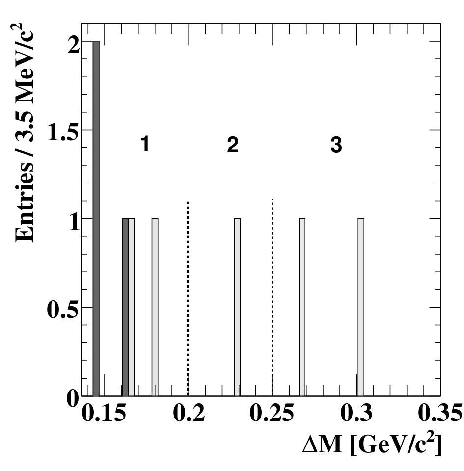
3 Current Experimental Results

3.1 Time-independent Experiments

3.1.1 Correlated decay results at 3.770 $\mathrm{\,Ge\kern-1.00006ptV}$

Using methods described in Section 2.1.1, the CLEO Collaboration reported the first measurement of the strong phase difference ${\delta_{K\pi}}$ in 2008.[31, 35]. From 281 $\mbox{\,pb}^{-1}$ of data collected at $\sqrt{s}=3.770~\mathrm{\,Ge\kern-1.00006ptV}$ with the CLEO-c detector, the correlated analysis was performed using different sets of external measurements as input. These included: measurements of two-body $D^{0}$ branching fractions; the previous, plus measurements of the time-integrated WS rate $R_{WS}\equiv\Gamma(D^{0}\rightarrow K^{+}\pi^{-})/\Gamma(D^{0}\rightarrow K^{-}\pi^{+})$ and the mixing rate $R_{M}$ (the “standard” fit); and the previous, plus measurements of $x$ , $y$ , ${x^{\prime}}^{2}$ , $y^{\prime}$ , and $r^{2}$ (the “extended” fit). Correlations between external inputs were incorporated in the fits. In the standard fit, $x\sin{\delta_{K\pi}}$ is fixed to zero. In the extended fit, this condition is relaxed.

Systematic uncertainties accounted for in the analyses included estimates of efficiencies for particle identification, reconstructing tracks, and for reconstructing neutral neutral decays ( $K^{0}_{\scriptscriptstyle S}$ and $\pi^{0}$ ). Other systematic uncertainties included efficiencies for $\eta$ reconstruction, selection cuts, fit model description, and detector and physics modeling. The largest systematics were for $\eta$ reconstruction (4.0%) and $\Delta E=E_{D^{0}}-E_{{\rm beam}}$ selection (0.5–5.0%). Bias estimates on the fitting procedure were obtained by studying a sample of simulated $D^{0}{\kern-1.60004pt\hbox{-}\kern 1.99997pt\overline{\kern-1.99997ptD}{}^{0}}$ decays fifteen times the size of the recorded dataset. Biases from the fitting procedure were less than one-half the size of the statistical errors on the fitted parameters.

Results from the standard and extended fits are given in Table 2. Likelihoods from the standard fit are shown in Fig. 17 and from the extended fit are shown in Fig. 18. The final result for ${\delta_{K\pi}}$ , including asymmetric errors estimated from the shape of the likelihood function shown in Fig. 17, is $\cos{\delta_{K\pi}}=1.03^{+0.31}_{-0.17}\pm 0.06$ . Limiting to the region $|\cos{\delta_{K\pi}}|<1$ , $|{\delta_{K\pi}}|<75^{\circ}$ at the 95% confidence level. From the extended fit, they obtain $\cos{\delta_{K\pi}}=1.10\pm 0.35\pm 0.07$ and $x\sin{\delta_{K\pi}}=(4.4^{+2.7}_{-1.8}\pm 2.9)\times 10^{-3}$ and ${\delta_{K\pi}}=(22^{+11}_{-12}{}^{+9}_{-11})^{\circ}$ . In both cases, the statistical errors were obtained by inspection of the log likelihood.

Table 2: CLEO mixing and

\delta_{K\pi}

strong phase difference measurements. From Refs. [31] and [35]. See text for fit descriptions.

\topruleParameter	Standard fit	Extended fit
\colrule $y$	$(-45\pm 59\pm 15)\times 10^{-3}$	$(6.5\pm 0.2\pm 2.1)\times 10^{-3}$
$x^{2}$	$(-1.5\pm 3.6\pm 4.2)\times 10^{-3}$	$(0.06\pm 0.01\pm 0.05)\times 10^{-3}$
$r^{2}$	$(8.0\pm 6.8\pm 1.9)\times 10^{-3}$	$(3.44\pm 0.01\pm 0.09)\times 10^{-3}$
$\cos{\delta_{K\pi}}$	$1.03^{+0.31}_{-0.17}\pm 0.06$	$1.10\pm 0.35\pm 0.07$
$x\sin{\delta_{K\pi}}$	Fixed at 0	$(4.4^{+2.7}_{-1.8}\pm 2.9)\times 10^{-3}$
${\delta_{K\pi}}$	—	$(22^{+11}_{-12}{}^{+9}_{-11})^{\circ}$
\botrule

In a recent preliminary analysis,[32] CLEO extended its quantum correlated coherent decay analysis to measure the strong phase differences in $D^{0}\rightarrow K^{+}\pi^{-}$ , $D^{0}\rightarrow K^{+}\pi^{-}\pi^{0}$ , $D^{0}\rightarrow K^{+}\pi^{-}\pi^{+}\pi^{-}$ and $D^{0}\rightarrow K^{0}_{S,L}h^{+}h^{-}$ , $h=\pi,K$ , using the full dataset ( $818\mbox{\,pb}^{-1}$ ) together with additional single- and double-tag modes. This analysis makes direct measurements of $r_{K\pi}^{2}$ and $\sin{\delta_{K\pi}}$ , resulting in approximately a factor of two smaller (and more symmetric) statistical uncertainties on $\cos{\delta_{K\pi}}$ . In the near future, BES-III will likely produce strong phase difference measurements with improved statistical precision.

3.2 Results from Time-dependent Analyses of Two-body Decays

3.2.1 $D^{0}\rightarrow K^{+}\pi^{-}$ Wrong-sign Decay Results

Several experiments, E691,[66] E791,[57] FOCUS,[67] CLEO,[68] BABAR,[69] and Belle[70] have set upper limits on $D^{0}{\kern-1.60004pt\hbox{-}\kern 1.99997pt\overline{\kern-1.99997ptD}{}^{0}}$ mixing by analyzing the time dependence of WS $D^{0}\rightarrow K^{+}\pi^{-}$ decays outlined in Sec. 2.2.1. Of these, the Belle limit, based on 400 $\mbox{\,fb}^{-1}$ , is the most stringent. Assuming $C\!P$ conservation, they find: ${x^{\prime}}^{2}<0.72\times 10^{-3}$ and $-9.9\times 10^{-3}<y^{\prime}<6.8\times 10^{-3}$ at the $95\%$ confidence level.

In 2007 the BABAR Collaboration reported evidence for $D^{0}{\kern-1.60004pt\hbox{-}\kern 1.99997pt\overline{\kern-1.99997ptD}{}^{0}}$ mixing from $(4030\pm 90)$ WS signal candidates and $(1141500\pm 1200)$ RS signal candidates in a $384\mbox{\,fb}^{-1}$ data sample. [12] The reconstructed decay-time distribution for WS data and the fit results with and without mixing (assuming $C\!P$ conservation) are shown in Fig. 19. The fit with mixing provides a substantially better description of the data than the fit with no mixing. The parameters obtained from fitting the BABAR data assuming $C\!P$ conservation are listed in Table 3.

In the BABAR measurement, the significance of the mixing signal is estimated from the change in the log likelihood, $-2\Delta\log{\cal L}{}$ , with respect to its value at the global minimum. Fig. 20 shows the confidence-level contours calculated using the change in log likelihood from the joint estimation of two parameters. The best fit value of the $({x^{\prime}}^{2},y^{\prime})$ parameters to the BABAR data is at the unphysical value of $({x^{\prime}}^{2}=-2.2\times 10^{-4},y^{\prime}=9.7\times 10^{-3})$ . As can be seen from Fig. 20, the two parameters are highly correlated with each other. Constraining the fit region to ${x^{\prime}}^{2}\geq 0$ yields $({x^{\prime}}^{2}=0,y^{\prime}=6.4\times 10^{-3})$ , and corresponds to $-2\Delta\log{\cal L}{}=0.7$ . The no-mix point corresponds to $-2\Delta\log{\cal L}{}=23.9$ statistical units. The maximum log likelihood is denoted as $\log{\cal L}{(}{x^{\prime}}^{2},y^{\prime})$ . Each systematic variation is included one at a time into the fit and a new log liklihood $\log{\cal L}{(}{x^{\prime}}^{2}_{i},y^{\prime}_{i})$ is obtained. The significance of the $i^{th}$ systematic variation is $s_{i}^{2}=2\left[\log{\cal L}{(}{x^{\prime}}^{2},y^{\prime})-\log{\cal L}{(}{x^{\prime}}^{2}_{i},y^{\prime}_{i})\right]/2.3$ , where the factor of 2.3 is the 68% confidence level for two degrees of freedom. Reducing $-2\Delta\log{\cal L}{}$ by $1+\sum_{i}s_{i}^{2}=1.3$ everywhere to account for systematic uncertainties results in a significance equivalent to 3.9 standard deviations. Predominant systematic uncertainties on the mixing parameters arise from modeling the long decay times of other charm decays populating the signal region and to a non-zero mean in the proper decay-time resolution function.

To allow for $CPV$ , the BABAR analysis fits the $D^{0}$ and $\kern 1.99997pt\overline{\kern-1.99997ptD}{}^{0}$ samples separately to determine the parameters $(R_{D}^{+},{x^{\prime+}}^{+^{2}},y^{\prime+})$ and $(R_{D}^{-},{x^{\prime-}}^{-^{2}},y^{\prime-})$ , respectively. From these fitted values, the parameters $R_{D}=\sqrt{R_{D}^{+}R_{D}^{-}}$ and $A_{D}=(R_{D}^{+}-R_{D}^{-})/(R_{D}^{+}+R_{D}^{-})$ are computed. The systematic component of the error on the BABAR measurement of $A_{D}$ is mainly due to uncertainties in modeling the slight asymmetry between the interactions of $K^{+}$ and $K^{-}$ mesons in the detector.

The CDF Collaboration, using a $1.5\mbox{\,fb}^{-1}$ data sample of $\bar{p}p$ collisions at $\sqrt{s}=1.96\mathrm{\,Te\kern-1.00006ptV}$ has shown evidence for mixing in the $D^{0}\rightarrow K^{+}\pi^{-}$ channel.[14] Since the CDF experiment was not running on the $\mathchar 28935\relax(4S)$ as BABAR and Belle were, removal of $B\rightarrow D$ decays was considerably more challenging than applying a simple center of mass momentum cut, as was done in the $B$ -factory measurements. On the other hand, due to the much larger average boost, the average flight distance in the lab is greater than in the $B$ -factory experiments. Despite the vastly different environment, the central values of the mixing parameters shown in Table 3 and the $({x^{\prime}}^{2},y^{\prime})$ C.L. contours shown in Fig. 21, both from the CDF experiment, agree remarkably well with the corresponding BABAR results. There is no evidence for $CPV$ from any of the reported measurements.

Table 3:

D^{0}{\kern-1.60004pt\hbox{-}\kern 1.99997pt\overline{\kern-1.99997ptD}{}^{0}}

mixing and

CPV

parameters from

D^{0}\rightarrow K^{+}\pi^{-}

decays. For results with two reported uncertainty components, the first is statistical and the second is systematic. The results with a single uncertainty component include both statistical and systematic uncertainties.

\topruleFit type	Parameter	Fit Results ( $/10^{-3}$ )
		BABAR[12]	CDF[14]	Belle[70]
\colruleNo $CPV$ or mixing	$R_{D}$	$3.53\pm 0.08\pm 0.04$	$4.15\pm 0.10$	$3.77\pm 0.08\pm 0.05$
\colruleNo $CPV$	$R_{D}$	$3.03\pm 0.16\pm 0.10$	$3.04\pm 0.55$	$3.64\pm 0.17$
	${x^{\prime}}^{2}$	$-0.22\pm 0.30\pm 0.21$	$-0.12\pm 0.35$	$0.18^{+0.21}_{-0.23}$
	$y^{\prime}$	$9.7\pm 4.4\pm 3.1$	$8.5\pm 7.6$	$0.6^{+4.0}_{-3.9}$
Significance		$3.9$	$3.8$	$2.0$
\colrule $CPV$ allowed	$R_{D}$	$3.03\pm 0.16\pm 0.10$	$-$	$-$
	$A_{D}$	$-21\pm 52\pm 15$	$-$	$23\pm 47$
	$A_{M}$	$-$	$-$	$670\pm 1200$
	${x^{\prime+}}^{+^{2}}$	$-0.24\pm 0.43\pm 0.30$	$-$	$-$
	$y^{\prime+}$	$9.8\pm 6.4\pm 4.5$	$-$	$-$
	${x^{\prime-}}^{-^{2}}$	$-0.20\pm 0.41\pm 0.29$	$-$	$-$
	$y^{\prime-}$	$9.6\pm 6.1\pm 4.3$	$-$	$-$
	${x^{\prime}}^{2}$	$-$	$-$	$<0.72$ (95% C.L.)
	$y^{\prime}$	$-$	$-$	$-28<y^{\prime}<21$ (95% C.L.)
\botrule

3.2.2 $D^{0}$ Lifetime Ratio Results

E791, FOCUS, CLEO, Belle, and BABAR have published $y_{CP}$ results [13, 42, 44, 45, 72, 73] from lifetime measurements of $D^{0}\rightarrow K^{+}K^{-}$ and $D^{0}\rightarrow\pi^{+}\pi^{-}$ decays relative to that from $D^{0}\rightarrow K^{-}\pi^{+}$ decays. Fits to the proper time distributions from the BABAR untagged analysis[45] are shown in Fig. 22. The lifetime measurement is determined from a fit using the decay time and decay-time error of candidates in a signal region, as described in Sec. 2.2.2. The charm background component shape and yield in the signal region are obtained from MC simulated events. The combinatorial background component shape in the signal region is estimated from sideband data. A fit to the $D^{0}$ data mass distribution is performed over the full mass range to estimate the total background and signal yields in the signal region. The combinatorial yield in the signal region is then obtained by subtracting the charm background yield from the total background yield there.

The results from the Belle and BABAR experiments on $A_{\Gamma}$ show no evidence for $C\!P$ violation. These measurements are shown at the bottom of Table 4. Results for $y_{CP}$ are shown in Fig. 23, and are given in Table 4. The Heavy Flavor Averaging Group (HFAG) world average $y_{CP}$ value[15, 71] is more than four standard deviations away from the no-mixing hypothesis ( $y_{CP}=0$ ).

Table 4: Results from

y_{CP}

(

\Delta\Gamma

) and

A_{\Gamma}

measurements from E791, FOCUS, CLEO, Belle, and BABAR experiments.[13, 42, 44, 45, 72, 73] Measurement uncertainties are given as statistical (first) and systematic (second). The world-average uncertainty is statistical and systematic combined.

\topruleExperiment	Parameter	Result (%)	data sample
\colruleE791[42]	$\Delta\Gamma$	$0.04\pm 0.14\pm 0.05$	500 $\mathrm{\,Ge\kern-1.00006ptV}$ $\pi$ N interactions ( $2\times 10^{10}$ events)
FOCUS[72]	$y_{CP}$	$3.42\pm 1.39\pm 0.74$	$\gamma$ N interactions ( $1\times 10^{6}$ reconstr. $D\rightarrow Kn(\pi)$
CLEO[73]	$y_{CP}$	$−1.2\pm 2.5\pm 1.4$	$9.0$ $\mbox{\,fb}^{-1}$ near $\mathchar 28935\relax(4S)$ resonance ; untagged
Belle[13]	$y_{CP}$	$−0.5\pm 1.0^{+0.7}_{-0.8}$	$23.4$ $\mbox{\,fb}^{-1}$ near $\mathchar 28935\relax(4S)$ resonance; untagged
Belle[13]	$y_{CP}$	$1.31\pm 0.32\pm 0.25$	$540$ $\mbox{\,fb}^{-1}$ near $\mathchar 28935\relax(4S)$ resonance ; $D^{*}$ tagged
Belle[13]	$y_{CP}$	$0.11\pm 0.61\pm 0.52$	$673$ $\mbox{\,fb}^{-1}$ near $\mathchar 28935\relax(4S)$ resonance ; $D\rightarrow(K^{+}K^{−})K^{0}$
BABAR[44]	$y_{CP}$	$1.03\pm 0.33\pm 0.19$	$384$ $\mbox{\,fb}^{-1}$ near $\mathchar 28935\relax(4S)$ resonance ; $D^{*}$ tagged
BABAR[45]	$y_{CP}$	$1.12\pm 0.26\pm 0.22$	$384$ $\mbox{\,fb}^{-1}$ near $\mathchar 28935\relax(4S)$ resonance ; untagged
BABAR[45]	$y_{CP}$	$1.16\pm 0.22\pm 0.18$	$D^{*}$ tagged + untagged combined
HFAG[71]	$y_{CP}$	$1.107\pm 0.217$	World Average
\botrule
Belle[13]	$A_{\Gamma}$	$0.01\pm 0.30\pm 0.15$	$540$ fb ${}^{−}1$ near $\mathchar 28935\relax(4S)$ resonance ; $D^{*}$ tagged
BABAR[44]	$A_{\Gamma}$	$0.26\pm 0.36\pm 0.08$	$384$ fb ${}^{−}1$ near $\mathchar 28935\relax(4S)$ resonance ; $D^{*}$ tagged
HFAG[71]	$A_{\Gamma}$	$0.123\pm 0.248$	World Average
\botrule

3.3 Results from Time-dependent Analyses of Multi-body Decays

3.3.1 $D^{0}\rightarrow K^{0}_{\scriptscriptstyle S}h^{+}h^{-}$ Analysis Results

CLEO[47], Belle[48, 74], and BABAR[46] have published results from time-dependent Dalitz-plot analyses of $D^{0}\rightarrow K^{0}_{\scriptscriptstyle S}\pi^{+}\pi^{-}$ decays and $D^{0}\rightarrow K^{0}_{\scriptscriptstyle S}K^{+}K^{-}$ (Belle, BABAR). The CLEO Collaboration, which pioneered this technique, set 95% confidence level (CL) limits on the mixing parameters $x$ and $y$ . Results for $x$ and $y$ are given in Table 5 and world averages in Fig. 25. No evidence for $C\!P$ violation has been seen by any of the experiments.

Table 5: Results for

x

y

, and

y_{CP}

from

D^{0}\rightarrow K^{0}_{\scriptscriptstyle S}\pi^{+}\pi^{-}

and

D^{0}\rightarrow K^{0}_{\scriptscriptstyle S}K^{+}K^{-}

time-dependent analyses. All results are from Dalitz-plot analyses except the Belle

y_{CP}

result. Uncertainties on

x

and

y

are statistical, experimental systematic, and resonance decay model systematic, respectively. From Refs. [46, 47, 48].

\topruleExperiment	Fit Type	Parameter	Result	95% C.L. Limit
\colruleCLEO[47]	No CPV	$x$ (%)	$1.8^{+3.4}_{-3.2}\pm 0.4\pm 0.4$	$(-4.7,8.6)$
CLEO[47]	No CPV	$y$ (%)	$-1.4^{+2.5}_{-2.4}\pm 0.8\pm 0.4$	$(-6.3,3.7)$
CLEO[47]	CPV	$x$ (%)	$2.3^{+3.5}_{-3.4}\pm 0.4\pm 0.4$	$(-4.5,9.3)$
CLEO[47]	CPV	$y$ (%)	$-1.5^{+2.5}_{-2.4}\pm 0.8\pm 0.4$	$(-6.4,3.6)$
Belle[48]	No CPV	$x$ (%)	$0.80\pm 0.29^{+0.09}_{-0.07}{}^{+0.10}_{-0.14}$	$(0.0,1.6)$
Belle[48]	No CPV	$y$ (%)	$0.33\pm 0.24^{+0.08}_{-0.12}{}^{+0.06}_{-0.08}$	$(-0.34,0.96)$
Belle[48]	CPV	$x$ (%)	$0.81\pm 0.30^{+0.10}_{-0.07}{}^{+0.09}_{-0.16}$	$\|x\|<1.6$
Belle[48]	CPV	$y$ (%)	$0.37\pm 0.25^{+0.07}_{-0.13}{}^{+0.07}_{-0.08}$	$\|y\|<1.04$
Belle[48]	CPV	$\|q/p\|$	$0.86^{+0.30}_{-0.29}{}^{+0.06}_{-0.03}\pm 0.08$	—
Belle[48]	CPV	$\arg(q/p)$ (^∘)	$14^{+16}_{-18}{}^{+5}_{-3}{}^{+2}_{-4}$	—
Belle[74]	No CPV	$y_{CP}(\%)$	$0.11\pm 0.61\pm 0.52$	—
BABAR[46]	No CPV	$x$ (%)	$0.16\pm 0.23\pm 0.12\pm 0.08$	—
BABAR[46]	No CPV	$y$ (%)	$0.57\pm 0.20\pm 0.13\pm 0.07$	—
\colruleWorld average[71]	No CPV	$x$ (%)	$0.419\pm 0.211$
	No CPV	$y$ (%)	$0.456\pm 0.186$
\botrule

Experimental systematics include variations in background and PDF models, efficiencies, event selection criteria, and experimental resolution effects. In addition to these, systematics from the chosen resonance decay model are evaluated as well.

Additional cross-checks are performed. Fitted values of background fractions, $D^{0}$ lifetimes, and decay-time scale factors are determined to be consistent with expectations or previous results. Decay-time distributions are shown in Fig. 24. Belle, CLEO, and BABAR perform additional mixing fits to check for $C\!P$ violation. BABAR performs separate fits to $D^{0}$ and $\kern 1.99997pt\overline{\kern-1.99997ptD}{}^{0}$ decays, and no evidence for $C\!P$ violation in mixing is seen. CLEO performs separate fits to $D^{0}$ and $\kern 1.99997pt\overline{\kern-1.99997ptD}{}^{0}$ samples. Belle incorporates additional $C\!P$ -violating parameters in their mixing fit. These additional fits yield results consistent with the nominal fitted values. No evidence for $C\!P$ violation is seen in any of the measurements.

3.3.2 $D^{0}\rightarrow K\pi\pi^{0}$ Analysis Results

The first observation of the WS decay mode $D^{0}\rightarrow K^{+}\pi^{-}\pi^{0}$ was reported by CLEO in 2001.[75] Using a 9 $\mbox{\,fb}^{-1}$ dataset of $e^{+}e^{-}$ collisions near the $\mathchar 28935\relax(4S)$ resonance, they observed the decay with a 4.9 standard deviation significance and reported a wrong-sign rate of $R_{WS}^{K\pi\pi^{0}}=[0.43^{+0.11}_{-0.10}\pm 0.07]\%$ . Using 281 $\mbox{\,fb}^{-1}$ of $e^{+}e^{-}$ colliding-beam data near the $\mathchar 28935\relax(4S)$ , Belle (2005) reported [49] a WS branching fraction of $R_{WS}^{K\pi\pi^{0}}=[0.229\pm 0.015^{+0.013}_{0.009}]\%$ . In 2006 BABAR reported [50] a measurement of $R_{WS}^{K\pi\pi^{0}}=[0.214\pm 0.008\pm 0.008]\%$ No evidence for $C\!P$ violation was observed in these studies.

BABAR analyzed the $D^{0}\rightarrow K\pi\pi^{0}$ decay mode using two different methods (see Sec. 2.3.2). Method I measured the time-integrated mixing rate $R_{M}=[0.023^{+0.018}_{-0.014}\pm 0.004]\%$ with a 95% CL upper limit of $R_{M}<0.054\%$ assuming $C\!P$ conservation. The result is compatible with the no-mixing hypothesis at the 4.5% CL. Additional results are given in Table 3.3.2. These include measurements allowing for $C\!P$ violation.

This study estimated systematic uncertainties by varying selection cuts, changing background PDF shapes and the decay-time resolution model, varying the $D^{0}$ lifetime, and changing efficiency corrections, and by performing the fit over the full Dalitz-plot phase space. Method I results are statistics-limited.

\toprule $C\!P$ conservation assumed	$C\!P$ violation allowed
\colrule BABAR method I [50]
$R_{M}=(0.023^{+0.018}_{-0.014}\pm 0.004)\%$	$R_{M}=(0.010^{+0.022}_{-0.007}\pm 0.003)\%$
$\alpha{\tilde{y}}^{\prime}=-0.012^{+0.006}_{-0.008}\pm 0.002$	$\alpha{\tilde{y}}^{\prime}\cos{\tilde{\phi}}=-0.012^{+0.006}_{-0.007}\pm 0.002$
	$\beta{\tilde{x}}^{\prime}\sin{\tilde{\phi}}=0.003^{+0.002}_{-0.005}\pm 0.000$
	$\|p/q\|=2.2^{+1.9}_{-1.0}\pm 0.1$
\colrule BABAR method II [53]
$x^{\prime}_{K\pi\pi^{0}}=\phantom{-}0.0261^{+0.0057}_{-0.0068}\pm 0.0039$	$x^{\prime+}_{K\pi\pi^{0}}=\phantom{-}0.0253^{+0.0054}_{-0.0063}\pm 0.0039$
$y^{\prime}_{K\pi\pi^{0}}=-0.0006^{+0.0055}_{-0.0064}\pm 0.0034$	$y^{\prime+}_{K\pi\pi^{0}}=-0.0005^{+0.0063}_{-0.0067}\pm 0.0050$
	$x^{\prime-}_{K\pi\pi^{0}}=\phantom{-}0.0355^{+0.0073}_{-0.0083}\pm 0.0065$
	$y^{\prime-}_{K\pi\pi^{0}}=-0.0054^{+0.0040}_{-0.0116}\pm 0.0041$
$r_{0}^{2}=(5.25^{+0.25}_{-0.31}\pm 0.12)\times 10^{-3}$
\botrule

	$\displaystyle\alpha\tilde{y}^{\prime}$	$\displaystyle\rightarrow$	$\displaystyle\|p/q\|^{\pm}(\alpha\tilde{y}^{\prime}\cos\tilde{\phi}\pm\beta\tilde{x}^{\prime}\sin\tilde{\phi}),$		(83)
	$\displaystyle x^{2}+y^{2}$	$\displaystyle\rightarrow$	$\displaystyle\|p/q\|^{\pm 2}(x^{2}+y^{2})$		(84)

	$\displaystyle R_{M}$	$\displaystyle=$	$\displaystyle[0.019{}^{+0.016}_{-0.015}({\rm stat.})\pm 0.002({\rm syst.})]\%,$		(85)
	$\displaystyle\alpha\tilde{y}^{\prime}$	$\displaystyle=$	$\displaystyle-0.006\pm{0.005}({\rm stat.})\pm 0.001({\rm syst.}),$		(86)

$\displaystyle R_{M}$	$\displaystyle=$	$\displaystyle[0.017{}^{+0.017}_{-0.016}({\rm stat.})\pm 0.003({\rm syst.})]\%,$	(87)
$\displaystyle\|p/q\|$	$\displaystyle=$	$\displaystyle 1.1{}^{+4.0}_{-0.6}({\rm stat.})\pm 0.1({\rm syst.}),$	(88)
$\displaystyle\alpha\tilde{y}^{\prime}\cos\tilde{\phi}$	$\displaystyle=$	$\displaystyle-0.006^{+0.008}_{-0.006}({\rm stat.})\pm 0.006({\rm syst.}),$	(89)
$\displaystyle\beta\tilde{x}^{\prime}\cos\tilde{\phi}$	$\displaystyle=$	$\displaystyle 0.002^{+0.005}_{-0.003}({\rm stat.})\pm 0.006({\rm syst.}).$	(90)

\topruleExperiment	$D^{0}$ modes	Results
\colruleE791[62]	$Ke\nu$	$R_{M}=(0.16^{+0.42}_{-0.37})$ %
	$K\mu\nu$	$R_{M}=(0.06^{+0.44}_{-0.40})$ %
	Combined	$R_{M}=0.11^{+0.30}_{-0.27}$ %
		$R_{M}<0.50\%$ at 90% CL
\colruleCLEO II.V[63]	$Ke\nu$	$R_{M}=(1.10\pm 0.76)$ % (stat.+syst. combined)
	$K^{*}e\nu$	$R_{M}=(\phantom{0}0.0\pm 0.31)$ % (stat.+syst. combined)
	Combined	$R_{M}=(0.16\pm 0.29)$ % (stat.+syst. combined)
\colruleBelle[61]	$K^{(*)}e\nu$	$R_{M}=(-0.6\pm 2.7^{+1.8}_{-2.1})\times 10^{-4}$
	$K^{(*)}\mu\nu$	$R_{M}=(5.9\pm 3.7^{+3.9}_{-4.5})\times 10^{-4}$
	Combined	$R_{M}=(1.3\pm 2.2\pm 2.0)\times 10^{-4}$
		$R_{M}<6.1\times 10^{-4}$ at 90% CL
\colruleBaBar singly tagged[65]	$K^{(*)}e\nu$	$R_{M}=0.0023\pm 0.0012\pm 0.0004$
		$R_{M}<0.0042$ at 90% CL
\colruleBaBar doubly tagged[64]	$K^{(*)}e\nu$	$R_{M}=0.4\times 10^{-4}$ (central value)
		$R_{M}$ in $(-2.2,2.8)\times 10^{-4}$ at 68% CL
		$R_{M}$ in $(-13,12)\times 10^{-4}$ at 90% CL
\botrule

Charm Meson Mixing: An Experimental Review

Abstract

keywords

PACS

1 Introduction

1.1 $D^{0}{\kern-1.60004pt\hbox{-}\kern 1.99997pt\overline{\kern-1.99997ptD}{}^{0}}$ Mixing Formalism

1.2 $C\!P$ violation

1.3 Outline

2 Analysis Techniques for Measuring Charm Mixing and CP Violation

2.1 Time-independent Methods

2.1.1 Correlated Decays at 3.770 $\mathrm{\,Ge\kern-1.00006ptV}$

2.2 Time-dependent Analyses of Two-body Decays

2.2.1 $D^{0}\rightarrow K^{+}\pi^{-}$ Wrong-sign Analysis

2.2.2 $D^{0}$ Lifetime Ratio Analysis

2.3 Time-dependent Analyses of Hadronic Multi-body Decay Modes

2.3.1 $D^{0}\rightarrow K^{0}_{\scriptscriptstyle S}h^{+}h^{-}$ Analysis

2.3.2 $D^{0}\rightarrow K^{+}\pi^{-}\pi^{0}$ Analysis

2.3.3 $D^{0}\rightarrow K^{+}\pi^{-}\pi^{+}\pi^{-}$ Analysis

2.3.4 Analysis of Wrong-sign Semileptonic Decays

3 Current Experimental Results

3.1 Time-independent Experiments

3.1.1 Correlated decay results at 3.770 $\mathrm{\,Ge\kern-1.00006ptV}$

3.2 Results from Time-dependent Analyses of Two-body Decays

3.2.1 $D^{0}\rightarrow K^{+}\pi^{-}$ Wrong-sign Decay Results

3.2.2 $D^{0}$ Lifetime Ratio Results

3.3 Results from Time-dependent Analyses of Multi-body Decays

3.3.1 $D^{0}\rightarrow K^{0}_{\scriptscriptstyle S}h^{+}h^{-}$ Analysis Results

3.3.2 $D^{0}\rightarrow K\pi\pi^{0}$ Analysis Results

3.3.3 $D^{0}\rightarrow K^{+}\pi^{-}\pi^{+}\pi^{-}$ Analysis Results

3.3.4 Semileptonic Decays Analysis Results

3.4 World Average Results

4 What’s Next?

4.1 BES-III

4.2 LHCb

4.3 SuperKEKB and Belle II

4.4 The Super Flavor Factory SuperB

5 Summary

Acknowledgments

References

\topruleParameter	No $CPV$	No direct $CPV$	$CPV$ -allowed
\colrule $x\ (\%)$	$0.65^{+0.18}_{-0.19}$	$0.63\pm 0.19$	$0.63^{+0.19}_{-0.20}$
$y\ (\%)$	$0.74\pm 0.12$	$0.75\pm 0.12$	$0.75\pm 0.12$
$\|q/p\|$	—	$1.02\pm 0.04$	$0.89^{+0.17}_{-0.15}$
$\varphi(^{\circ})$	—	$-1.05^{+1.89}_{-1.94}$	$-10.1^{+9.4}_{-8.8}$
\botrule

Charm Meson Mixing: An Experimental Review

Abstract

keywords

PACS

1 Introduction

1.1 D0-D¯0D^{0}{\kern-1.60004pt\hbox{-}\kern 1.99997pt\overline{\kern-1.99997ptD}{}^{0}} Mixing Formalism

1.2 C​PC\!P violation

1.3 Outline

2 Analysis Techniques for Measuring Charm Mixing and CP Violation

2.1 Time-independent Methods

2.1.1 Correlated Decays at 3.770 Ge​V\mathrm{\,Ge\kern-1.00006ptV}

2.2 Time-dependent Analyses of Two-body Decays

2.2.1 D0→K+​π−D^{0}\rightarrow K^{+}\pi^{-} Wrong-sign Analysis

2.2.2 D0D^{0} Lifetime Ratio Analysis

2.3 Time-dependent Analyses of Hadronic Multi-body Decay Modes

2.3.1 D0→KS0​h+​h−D^{0}\rightarrow K^{0}_{\scriptscriptstyle S}h^{+}h^{-} Analysis

2.3.2 D0→K+​π−​π0D^{0}\rightarrow K^{+}\pi^{-}\pi^{0} Analysis

2.3.3 D0→K+​π−​π+​π−D^{0}\rightarrow K^{+}\pi^{-}\pi^{+}\pi^{-} Analysis

2.3.4 Analysis of Wrong-sign Semileptonic Decays

3 Current Experimental Results

3.1 Time-independent Experiments

3.1.1 Correlated decay results at 3.770 Ge​V\mathrm{\,Ge\kern-1.00006ptV}

3.2 Results from Time-dependent Analyses of Two-body Decays

3.2.1 D0→K+​π−D^{0}\rightarrow K^{+}\pi^{-} Wrong-sign Decay Results

3.2.2 D0D^{0} Lifetime Ratio Results

3.3 Results from Time-dependent Analyses of Multi-body Decays

3.3.1 D0→KS0​h+​h−D^{0}\rightarrow K^{0}_{\scriptscriptstyle S}h^{+}h^{-} Analysis Results

3.3.2 D0→K​π​π0D^{0}\rightarrow K\pi\pi^{0} Analysis Results

3.3.3 D0→K+​π−​π+​π−D^{0}\rightarrow K^{+}\pi^{-}\pi^{+}\pi^{-} Analysis Results

3.3.4 Semileptonic Decays Analysis Results

3.4 World Average Results

4 What’s Next?

4.1 BES-III

4.2 LHCb

4.3 SuperKEKB and Belle II

4.4 The Super Flavor Factory SuperB

5 Summary

Acknowledgments

References

1.1 $D^{0}{\kern-1.60004pt\hbox{-}\kern 1.99997pt\overline{\kern-1.99997ptD}{}^{0}}$ Mixing Formalism

1.2 $C\!P$ violation

2.1.1 Correlated Decays at 3.770 $\mathrm{\,Ge\kern-1.00006ptV}$

2.2.1 $D^{0}\rightarrow K^{+}\pi^{-}$ Wrong-sign Analysis

2.2.2 $D^{0}$ Lifetime Ratio Analysis

2.3.1 $D^{0}\rightarrow K^{0}_{\scriptscriptstyle S}h^{+}h^{-}$ Analysis

2.3.2 $D^{0}\rightarrow K^{+}\pi^{-}\pi^{0}$ Analysis

2.3.3 $D^{0}\rightarrow K^{+}\pi^{-}\pi^{+}\pi^{-}$ Analysis

3.1.1 Correlated decay results at 3.770 $\mathrm{\,Ge\kern-1.00006ptV}$

3.2.1 $D^{0}\rightarrow K^{+}\pi^{-}$ Wrong-sign Decay Results

3.2.2 $D^{0}$ Lifetime Ratio Results

3.3.1 $D^{0}\rightarrow K^{0}_{\scriptscriptstyle S}h^{+}h^{-}$ Analysis Results

3.3.2 $D^{0}\rightarrow K\pi\pi^{0}$ Analysis Results

3.3.3 $D^{0}\rightarrow K^{+}\pi^{-}\pi^{+}\pi^{-}$ Analysis Results

References

- [1] Amitava Datta and Dharmadas Kumbhakar. - Mixing: A Possible Test of Physics Beyond the Standard Model. Z.Phys., C27:515, 1985.
- [2] Alexey A. Petrov. On dipenguin contribution to mixing. Phys.Rev., D56:1685–1687, 1997.
- [3] Eugene Golowich and Alexey A. Petrov. Short distance analysis of mixing. Phys.Lett., B625:53–62, 2005. 14 pages, 1 figure, 2 tables, revtex Report-no: WSU-HEP-0503.
- [4] Howard Georgi. mixing in heavy quark effective field theory. Phys.Lett., B297:353–357, 1992.
- [5] Thorsten Ohl, Giulia Ricciardi, and Elizabeth H. Simmons. mixing in heavy quark effective field theory: The Sequel. Nucl.Phys., B403:605–632, 1993.
- [6] Ikaros I.Y. Bigi and Nikolai G. Uraltsev. oscillations as a probe of quark hadron duality. Nucl.Phys., B592:92–106, 2001.
- [7] Adam F. Falk, Yuval Grossman, Zoltan Ligeti, Yosef Nir, and Alexey A. Petrov. The mass difference from a dispersion relation. Phys.Rev., D69:114021, 2004.
- [8] Adam F. Falk, Yuval Grossman, Zoltan Ligeti, and Alexey A. Petrov. SU(3) breaking and mixing. Phys.Rev., D65:054034, 2002.
- [9] Harry N. Nelson. Compilation of mixing predictions. 1999. International Symposium on Lepton and Photon Interactions at High Energies, arXiv:hep-ex/9908021.
- [10] Alexey A Petrov. Charm mixing in the Standard Model and beyond. Int.J.Mod.Phys., A21:5686–5693, 2006.
- [11] Eugene Golowich, JoAnne Hewett, Sandip Pakvasa, and Alexey A. Petrov. Implications of Mixing for New Physics. Phys.Rev., D76:095009, 2007.
- [12] Bernard Aubert et al. Evidence for Mixing. Phys.Rev.Lett., 98:211802, 2007.
- [13] M. Staric et al. Evidence for Mixing. Phys.Rev.Lett., 98:211803, 2007.
- [14] T. Aaltonen et al. Evidence for mixing using the CDF II Detector. Phys.Rev.Lett., 100:121802, 2008.
- [15] D. Asner et al. Averages of -hadron, -hadron, and -lepton Properties. 2010. arXiv:1010.1589 [hep-ex].
- [16] John F. Donoghue, Eugene Golowich, Barry R. Holstein, and Josip Trampetic. Dispersive Effects in Mixing. Phys.Rev., D33:179, 1986.
- [17] Ikaros I. Bigi and A. I Sanda. CP Violation. Cambridge University Press, New York, 2009. ISBN: 978-0-521-84794-0.
- [18] P. K. Kabir. The Puzzle: Strange Decays of the Neutral Kaon. Academic Press, Inc., 111 Fifth Avenue, New York, New York 10003, 1968. EAN: 978-0-123-93150-4.
- [19] K Nakamura et al. Review of particle physics. J.Phys.G, G37:075021, 2010.
- [20] Yosef Nir. violation in and beyond the standard model. 1999. arXiv:hep-ph/9911321.
- [21] Yosef Nir. violation in meson decays. pages 79–145, 2005. arXiv:hep-ph/0510413.
- [22] Alexander L. Kagan and Michael D. Sokoloff. On Indirect Violation and Implications for and - mixing. Phys.Rev., D80:076008, 2009.
- [23] F. Buccella, Maurizio Lusignoli, G. Miele, A. Pugliese, and Pietro Santorelli. Nonleptonic weak decays of charmed mesons. Phys.Rev., D51:3478–3486, 1995.
- [24] S. Bianco, F.L. Fabbri, D. Benson, and I. Bigi. A Cicerone for the physics of charm. Riv.Nuovo Cim., 26N7:1–200, 2003. Supersedes hep-ex/0306039.
- [25] Alexey A. Petrov. Hunting for violation with untagged charm decays. Phys.Rev., D69:111901, 2004.
- [26] Makoto Kobayashi and Toshihide Maskawa. CP Violation in the Renormalizable Theory of Weak Interaction. Prog.Theor.Phys., 49:652–657, 1973.
- [27] ed. Harrison, P.F. and ed. Quinn, Helen R. The BABAR physics book: Physics at an asymmetric factory. 1998. SLAC-R-0504.
- [28] Matthew Charles. Mixing and -violation studies in charm decays at LHCb. 2011. arXiv:1112.4155 [hep-ex].
- [29] Joachim Brod, Alexander L. Kagan, and Jure Zupan. On the size of direct violation in singly Cabibbo-suppressed decays. 2011.
- [30] Yuval Grossman, Alexander L. Kagan, and Yosef Nir. New physics and violation in singly Cabibbo suppressed decays. Phys.Rev., D75:036008, 2007.
- [31] J.L. Rosner et al. Determination of the Strong Phase in Using Quantum-Correlated Measurements. Phys.Rev.Lett., 100:221801, 2008.
- [32] Werner M. Sun. Quantum correlations in charm decays. Conf.Proc., C100901:58–64, September 2010. Physics in Collision (PIC2010).
- [33] Maurice Goldhaber and Jonathan L. Rosner. Mixing of Neutral Charmed Mesons and Tests for Violation in their Decays. Phys.Rev., D15:1254, 1977.
- [34] Michael Gronau, Yuval Grossman, and Jonathan L. Rosner. Measuring — mixing and relative strong phases at a charm factory. Phys.Lett., B508:37–43, 2001.
- [35] David Mark Asner et al. Determination of the Relative Strong Phase Using Quantum-Correlated Measurements in at CLEO. Phys. Rev., D78:012001, 2008.
- [36] T. E. Coan et al. Absolute Branching Fraction Measurements of Exclusive Semileptonic Decays. Phys. Rev. Lett., 95:181802, 2005.
- [37] Q. He et al. Comparison of and Decay Rates. Phys. Rev. Lett., 100:091801, 2008.
- [38] Werner M. Sun. Simultaneous least squares treatment of statistical and systematic uncertainties. Nucl. Instrum. Meth., A556:325–330, 2006.
- [39] D. M. Asner and W. M. Sun. Time-Independent Measurements of - Mixing and Relative Strong Phases Using Quantum Correlations. Phys. Rev., D73:034024, 2006.
- [40] D. M. Asner and W. M. Sun. Erratum: Time-Independent Measurements of - Mixing and Relative Strong Phases Using Quantum Correlations [Phys. Rev. D 73, 034024 (2006). Phys. Rev., D77:019901, 2008.
- [41] Tie-hui (Ted) Liu. The mixing search: Current status and future prospects. 1994.
- [42] E. M. Aitala et al. Measurements of lifetimes and a limit on the lifetime difference in the neutral meson system. Phys. Rev. Lett., 83:32–36, 1999.
- [43] Sven Bergmann, Yuval Grossman, Zoltan Ligeti, Yosef Nir, and Alexey A. Petrov. Lessons from CLEO and FOCUS Measurements of - Mixing Parameters. Phys. Lett., B486:418–425, 2000.
- [44] Bernard Aubert et al. Measurement of - mixing using the ratio of lifetimes for the decays , , and . Phys. Rev., D78:011105(R), 2008.
- [45] Bernard Aubert et al. Measurement of - Mixing using the Ratio of Lifetimes for the Decays and . Phys. Rev., D80:071103(R), 2009.
- [46] P. del Amo Sanchez et al. Measurement of - mixing parameters using and decays. Phys.Rev.Lett., 105:081803, 2010.
- [47] D.M. Asner et al. Search for mixing in the Dalitz plot analysis of . Phys.Rev., D72:012001, 2005.
- [48] L.M. Zhang et al. Measurement of - mixing in decays. Phys.Rev.Lett., 99:131803, 2007.
- [49] X. C. Tian et al. Measurement of the wrong-sign decays and search for violation. Phys. Rev. Lett., 95:231801, 2005.
- [50] Bernard Aubert et al. Search for - Mixing and Branching-Ratio Measurement in the Decay . Phys. Rev. Lett., 97:221803, 2006.
- [51] Muriel Pivk and Francois R. Le Diberder. SPlot: A Statistical tool to unfold data distributions. Nucl.Instrum.Meth., A555:356–369, 2005.
- [52] Paul E. Condon and Paul L. Cowell. Channel Likelihood: An Extension of Maximum Likelihood for Multibody Final States. Phys.Rev., D9:2558, 1974.
- [53] Bernard Aubert et al. Measurement of - mixing from a time-dependent amplitude analysis of decays. Phys. Rev. Lett., 103:211801, 2009.
- [54] S. Kopp et al. Dalitz analysis of the decay . Phys. Rev., D63:092001, 2001.
- [55] D. Aston, N. Awaji, T. Bienz, F. Bird, J. D’Amore, et al. A Study of Scattering in the Reaction at 11-. Nucl.Phys., B296:493, 1988.
- [56] G. Goldhaber, J. Wiss, G.S. Abrams, M.S. Alam, A. Boyarski, et al. and Meson Production Near 4-GeV in Annihilation. Phys.Lett., B69:503, 1977.
- [57] E.M. Aitala et al. A Search for - mixing and doubly Cabibbo suppressed decays of the in hadronic final states. Phys.Rev., D57:13–27, 1998.
- [58] S.A. Dytman et al. Evidence for the decay . Phys.Rev., D64:111101, 2001.
- [59] J.J. Aubert et al. Observation of Wrong Sign Trimuon Events in 250-GeV Muon - Nucleon Interactions. Phys.Lett., B106:419, 1981.
- [60] A. Bodek, R. Breedon, R.N. Coleman, William L. Marsh, S. Olsen, et al. Limits on - Mixing and Bottom Particle Production Cross-Sections from Hadronically Produced Same Sign Dimuon Events. Phys.Lett., B113:82, 1982.
- [61] U. Bitenc et al. Improved search for mixing using semileptonic decays at Belle. Phys. Rev., D77:112003, 2008.
- [62] E. M. Aitala et al. Search for - mixing in semileptonic decay modes. Phys. Rev. Lett., 77:2384–2387, 1996.
- [63] C. Cawlfield et al. Limits on neutral mixing in semileptonic decays. Phys. Rev., D71:077101, 2005.
- [64] Bernard Aubert et al. Search for - mixing using doubly flavor tagged semileptonic decay modes. Phys. Rev., D76:014018, 2007.
- [65] Bernard Aubert et al. Search for - mixing using semileptonic decay modes. Phys. Rev., D70:091102, 2004.
- [66] J.C. Anjos et al. A Study of Mixing. Phys.Rev.Lett., 60:1239, 1988.
- [67] J.M. Link et al. Measurement of the doubly Cabibbo suppressed decay and a search for charm mixing. Phys.Lett., B618:23–33, 2005.
- [68] R. Godang et al. Search for mixing. Phys.Rev.Lett., 84:5038–5042, 2000.
- [69] Bernard Aubert et al. Search for mixing and a measurement of the doubly Cabibbo-suppressed decay rate in decays. Phys.Rev.Lett., 91:171801, 2003.
- [70] L.M. Zhang et al. Improved constraints on mixing in decays at BELLE. Phys.Rev.Lett., 96:151801, 2006.
- [71] Heavy Flavor Averaging Group. Charm physics results. http://www.slac.stanford.edu/xorg/hfag/charm/index.html.
- [72] J. M. Link et al. A measurement of lifetime differences in the neutral meson system. Phys. Lett., B485:62–70, 2000.
- [73] S. E. Csorna et al. Lifetime Differences, direct Violation and Partial Widths in Meson Decays to and . Phys. Rev., D65:092001, 2002.
- [74] A. Zupanc et al. Measurement of in meson decays to the final state. Phys. Rev., D80:052006, 2009.
- [75] G. Brandenburg et al. Rate measurement of and constraints on - mixing. Phys. Rev. Lett., 87:071802, 2001.
- [76] Bernard Aubert et al. Search for mixing in the decays . 2006. arXiv:hep-ex/0607090.
- [77] R. Aaij et al. Measurement of mixing and violation parameters in two-body charm decays. 2011. arXiv:1112.4698 [hep-ex].
- [78] Yangheng Zheng. Current and Future Charm Experiments. 2011. arXiv:1102.4502 [hep-ex].
- [79] Marco Gersabeck. Searches for Violation in Charm Mixing at LHCb. September 2010. Presented at 6th International Workshop on the CKM Unitarity Triangle, Warwick, UK.
- [80] Philip John Hunt. Results and prospects for charm physics at LHCb. PoS, KRUGER2010:061, 2011.
- [81] R. Aaij et al. Evidence for violation in time-integrated decay rates. 2011. arXiv:1112.0938 [hep-ex].
- [82] Henryk Palka. Status of Super-KEKB and Belle II. Acta Phys.Polon., B41:2595–2604, 2010.
- [83] T. Aushev. Status and prospects of SuperKEKB collider and Belle II experiment. 2012. arXiv:1201.1248 [hep-ex].
- [84] T. Abe et al. Belle II Technical Design Report. 2010. arXiv:1011.0352 [physics.ins-det].
- [85] B. O’Leary et al. SuperB Progress Reports – Physics. 2010. arXiv:1008.1541 [hep-ex].