The potential of the effective Polyakov line action from the underlying lattice gauge theory
Abstract
I adapt a numerical method, previously applied to investigate the Yang-Mills vacuum wavefunctional, to the problem of extracting the effective Polyakov line action from SU() lattice gauge theories, with or without matter fields. The method can be used to find the variation of the effective Polyakov line action along any trajectory in field configuration space; this information is sufficient to determine the potential term in the action, and strongly constrains the possible form of the kinetic term. The technique is illustrated for both pure and gauge-Higgs SU(2) lattice gauge theory at finite temperature. A surprise, in the pure gauge theory, is that the potential of the corresponding Polyakov line action contains a non-analytic (yet center-symmetric) term proportional to , where is the trace of the Polyakov line at a given point, in addition to the expected analytic terms proportional to even powers of .
Keywords:
Confinement,lattice gauge theoriespacs
11.15.Ha, 12.38.AwI Introduction
Consider a lattice gauge theory with gauge group SU() on a periodic lattice of time extent , possibly containing matter fields and a chemical potential. If we integrate out all degrees of freedom under the constraint that Polyakov line holonomies are held fixed, then the resulting distribution depends only on those Polyakov line holonomies or, more precisely, on their eigenvalues. The logarithm of this distribution is defined to be the effective Polyakov line action .
If the underlying lattice gauge theory in dimensions has a sign problem due to a non-zero chemical potential, then probably also has a sign problem. However, there are indications that the sign problem may be more tractable in than in the underlying theory. Using strong-coupling and hopping parameter expansions, it is possible to actually carry out the integrations over gauge and matter fields mentioned above, to arrive at an action of the form 11 1 This is the action at leading order. For the effective action determined at higher orders in the combined strong-coupling and hopping parameter expansions, cf. [1].
| (1) |
where are calculable constants depending on the gauge coupling, quark masses, and temperature in the underlying theory. To minimize minus signs later on, the overall sign of is defined such that the Boltzmann weight is proportional to , rather than . The Polyakov line holonomies SU() in (1) are also known as “effective spins.” A path integral based on an effective spin action of the form (1), for a wide range of , can be treated by a number of different methods, including the “flux representation” [2], reweighting [1], and stochastic quantization [3]. Even traditional mean field methods have had some degree of success in determining the phase diagram [4].
The problem, of course, is that strong lattice coupling and heavy quark masses lie outside the parameter range of phenomenological interest, and it is not obvious how to extract for parameters inside the range of interest, even at . There have been some efforts in this direction, notably the inverse Monte Carlo method of ref. [5, *Heinzl:2005xv], as well as early studies [7, 8] which employed microcanonical and Migdal-Kadanoff methods, respectively. There is also a strategy for determining the phase structure of lattice gauge theory from an effective spin theory, whose form is suggested by high-order strong-coupling and hopping parameter expansions [1]. Here, however, I will discuss a different approach to the problem, recently suggested in ref. [4], which will be illustrated for SU(2) pure gauge and gauge-Higgs theories.
II The “Relative Weights” Approach
Let be the lattice QCD action at temperature in lattice units, with lattice gauge coupling , and a set of quark masses denoted collectively . We set chemical potential for now. It is convenient to impose a temporal gauge condition in which the timelike link variables are set to the unit matrix everywhere except on a single time slice, say at . In that case, is the Polyakov line holonomy passing through the site . The effective Polyakov line action is defined in terms of the partition function
| (2) | |||||
or equivalently
| (3) |
Because temporal gauge has a residual symmetry under time-independent gauge transformations, it follows that is invariant under , which means that only depends on the eigenvalues of the Polyakov line holonomies.
Now consider a finite set of SU() “effective spin” configurations in the three-dimensional cubic lattice of volume ,
| (4) |
Each member of the set can be used to specify the timelike links on the timeslice . Define
| (5) |
and consider the ratio
| (6) | |||||
where in the second line we have merely divided both the numerator and denominator by a common factor. However, by inserting this factor, both the numerator and denominator acquire a meaning in statistical mechanics, because the factor can be interpreted as the partition function of a system in which the configuration of timelike link variables at is restricted to belong to the set . This means that
| (7) |
is simply the probability, in this statistical system, for the -th configuration to be found on the timeslice. This probability can be determined from a slightly modified Monte Carlo simulation of the original lattice action. The simulation proceeds by standard algorithms, for all degrees of freedom other than the timelike links at , which are held fixed. Periodically, on the timeslice, one member of the given set of timelike link configurations is selected by the Metropolis algorithm, and all timelike links on that timeslice are updated simultaneously. Let be the number of times that the -th configuration is selected by the algorithm, and . Then is given by
| (8) |
and this in turn gives us the relative weights
| (9) |
for all elements of the set. A computation of this kind allows us to test any specific proposal for , which may be motivated by some theoretical considerations. But it might also be possible, given data on the relative weights of a variety of different sets, to guess the action that would lead to these results. In this article we will consider sets of spatially constant Polyakov line configurations, and small plane wave perturbations around a constant background. This is already sufficient to determine the potential term in , and to suggest the form of the full action.
The method described above was proposed long ago [9] in connection with the Yang-Mills vacuum wavefunctional. Recently there have been some sophisticated suggestions for the form of this wavefunctional in 2+1 dimensions, and the technique was revived in order to test these ideas in ref. [10]. The main difference between the method as applied to vacuum wavefunctionals, and as applied to determining , is that in the former case the simulation chooses from a fixed set of spacelike link configurations on the timeslice, while in the latter the choice is made from a set of timelike link configurations.
II.1 Finite chemical potential
Let denote the QCD action with a chemical potential, which can be obtained from by the following replacement of timelike links at :
| (10) |
The corresponding Polyakov line action is in principle obtained from (3), with as the underlying action. Of course the integration indicated in (3) can so far only be carried out for strong couplings and large quark masses, but it is not hard to see that each contribution to in the strong-coupling + hopping parameter expansion at maps into a corresponding contribution to by the replacement
| (11) |
It is reasonable then to suppose that this mapping holds in general, i.e. if we have by some means obtained beyond the range of validity of the strong-coupling + hopping parameter expansion, then the corresponding is obtained by making the change of variables (11). There is, however, a possible source of ambiguity in this scheme (noted in [4]), coming from identities such as
| (12) |
in SU(3). One way around this ambiguity is to enlarge the range of , allowing these variables to take on values
| (13) |
where is an element of N. In other words, we allow the links to take on values in the group, although it will be sufficient for our purposes to let be -independent.22 2 It is also sufficient to restrict to . The full range is redundant, because of the center of SU(). Suppose we are able to determine for this enlarged domain of Polyakov line variables. Then is obtained by analytic continuation, .
The essential point here is that if one can determine by simulations of at , then this result can be used to determine at finite chemical potential. If the sign problem is in fact tractable for , as recent results seem to suggest, then this may be a useful way of attacking the sign problem in full QCD.
II.2 Relative weights, and path-derivatives of
Let be the configuration space of effective spins on an lattice, and let the variable parametrize some path through . The method of relative weights is particularly useful in computing derivatives of the Polyakov line action
| (14) |
along the path. To see this, we begin by taking the logarithm of both sides of eq. (9), and find
| (15) | |||||
(From this point on we will drop the limit.) Now imagine parametrizing the effective spins by a parameter ; each value of gives us a different configuration . Let the configuration correspond to , and correspond to . Then
| (16) |
However, rather than using only two configurations to compute the derivative, we can obtain a more accurate numerical estimate if we let increase in increments of , e.g.
| (17) |
and use all of the values obtained for in the simulation. For small enough, the data for vs. will fit a straight line, and then we obtain the estimate
| (18) |
The procedure will be illustrated explicitly in the next section.
III Testing the method at strong coupling
The first step is to compute for a case where we know the answer analytically. As mentioned previously, can be readily computed in the strong-coupling + hopping parameter expansion. We will consider here the case of pure SU(2) Yang-Mills theory at a strong coupling . If the lattice is lattice spacings in the time direction, then computing the diagrammatic contributions to at leading and next-to-leading order in the strong-coupling/character expansion we find
| (19) | |||||
where
| (20) |
Let us first consider sets of spatially constant configurations with varying amplitudes in the neighborhood of , i.e.
| (21) |
so in this case is the parameter of the previous section. If we divide into a kinetic and potential part, which in the case of (19) is
| (22) |
then is giving us the derivative of the potential piece, which can then be reconstructed, up to an irrelevant constant, by integration. So the procedure for determining (assuming it were not already known from the strong-coupling expansion) is to compute numerically, fit the results to some appropriate polynomial in , and then integrate the fit.
Our sample simulation is carried out in pure SU(2) lattice gauge theory at coupling (well within the regime of strong couplings) on a lattice with sets of spatially constant configurations. Figure 1 shows the data for plotted vs. spatial lattice volume (), at . It is clear that the data falls quite accurately on a straight line, and the slope gives an estimate for the derivative
| (23) |
which can be compared to the value obtained from the strong-coupling expansion. The derivative obtained from numerical simulation vs. is plotted in Fig. 2, and it obviously fits a straight line. Therefore the potential is quadratic in , and we find, at
where we have dropped, in the upper line, an irrelevant constant of integration. The small numerical difference between the relative weights and strong-coupling results can probably be attributed to neglected higher order terms in the strong-coupling expansion.33 3 Statistical errors are estimated from best fit slopes obtained from eight independent runs. Where errorbars are not shown explicitly, in the two-dimensional plots shown below, they are smaller than the symbol size.


In order to investigate the kinetic term, we consider plane-wave deformations of spatially constant configurations. The path through configuration space is again parametrized by , with
| (28) |
where the are integers, not all of which are zero. For this class of configurations we have, for the action (19)
| (29) |
Since the deformation of the action is proportional to , it is natural to consider the derivative of with respect to , i.e.
| (30) |
and therefore we can choose to let , rather than , increase in equal increments, so that .

The numerical procedure is similar to the determination of the potential term: we compute the derivative , at fixed and , from the slope of a plot of vs. . Then these values for the derivative are plotted, at various values of , against squared lattice momentum
| (31) |
The result, at , is shown in Fig. 3, and we find, for a trajectory (28) at fixed ,
| (32) |
where
| (33) |
The simulation has also been carried out at other values of , but the results are almost indistinguishable from Fig. 3, and so are not displayed here. The important point, however, is that the path derivative (32) is independent.
Integrating with respect to , we find that along any path parametrized by with fixed
| (34) |
where is a constant of integration, which can be determined from the data on the potential:
| (35) |
The next step is to express along the path in terms of (or ). From the definitions (28), (31), one easily finds that (34) can be expressed as
| (36) |
The constants and are, within statistical error, consistent with zero. So we will just drop these terms. Then along the trajectory the action has the form
| (37) |
and of course the natural conjecture is that this is the action itself, at any point in configuration space. Further checks would be to calculate numerical derivatives along other trajectories, to test the consistency of this conjecture. We don’t really need to do that here, since the action at strong couplings is already known analytically, and is given in eq. (19) to leading and next-to-leading order in the strong-coupling expansion. At we have, from eq. (19), that
| (38) |
which is a close match to what we have arrived at via the relative weights procedure.
This is, perhaps, a lot of effort to derive a known result. We have gone through this exercise in order to illustrate the method, and to make sure, in a case where the answer is known, that the method actually works.
IV Potential in pure-gauge theory, weaker couplings
We now reduce the lattice coupling of the underlying SU(2) pure-gauge theory, setting with inverse temperature in lattice units. At this coupling and temperature (which is still inside the confinement phase of the theory), the effective Polyakov line action is not known.
The easiest task is to determine the potential part of the action. For the purposes of this article, we define the kinetic part of the action to be the piece which vanishes for spatially constant configurations, while the potential part is local. With these definitions
| (39) |
and the function is determined by evaluating on configurations which are constant in 3-space, i.e.
| (40) |
Then by definition the kinetic part of the action is
| (41) |
In order to determine , we consider as before the path through configuration space (21) parametrized by the variable , and once again we can identify with as in (23). The derivatives are determined by the relative weight method described above, the dependence on is fit to a polynomial, and is then determined, up to an irrelevant constant, by integration over .
Because the center symmetry is unbroken at and , and is a class function, it is natural to assume that is well represented by a few group characters of zero N-ality ( integer for SU(2)), and the potential is analytic in . Surprisingly, this is not what is found.
Figure 4(a) shows the data for the derivative
| (42) | |||||
at on a volume, which, as in the strong-coupling case, extrapolates linearly to zero at . Also shown is a best fit of to the polynomial
| (43) |
with the best fit constants shown in Table 1. What is initially a little troubling about this fit is that upon integration, and up to an irrelevant integration constant, we must have
| (44) |
which appears to violate center symmetry, i.e. for SU(2) gauge theory. Because of center symmetry, the character expansion of contains only characters with integer. It is a property of the SU(2) group characters that each can be expressed as a polynomial of order in , containing only even powers of for integer, and only odd powers for half-integer. Then if the character expansion of is truncated at some , the -derivative is a polynomial in odd powers of up to .


One might expect that can be accurately approximated by a handful of group characters. However, the attempt to fit the data with only a few odd powers of is unsuccessful, in the sense that each of the three fitting functions
corresponding to truncated character expansions with , respectively, gives an unacceptable fit, as seen in Fig. 4(b). The reduced values in the three cases are , respectively. This is to be compared to the reduced for the fitting function (43).
| Potential fit | ||
|---|---|---|
| 4.61(2) | 1.77(8) | |
All this seems to imply that has a term violating center symmetry, but of course that cannot be the case. In order that is an even function of , it must be that the derivative is an odd function, , which in turn means that the coefficient of the quadratic term in (43) must change sign when . This is easy to check; we simply repeat the calculation with in (21), with the result shown in 4(c). Here the squares are the data for at , while the circles are data for at . The fact that the corresponding data points at lie on top of each other means that the derivative is an odd function, and the potential itself is an even function of , as it must be. The conclusion, which follows from the best fit, is that over the full range the potential, up to an irrelevant constant, is given by
| (49) |
This function is non-analytic, because of the absolute value, but still center symmetric, with the constants given in Table 1. It should be emphasized again that this potential cannot be approximated very well by a simple sum of SU(2) group characters. Of course, any class function (including ) can be approximated by a sufficiently large number of group characters, just as a step function can be approximated by a truncated Fourier series. But keeping only a relatively small number of group characters introduces “wiggles” in the approximation to the potential (which are seen in Fig. 4(b)) much like the truncated Fourier series does for the step function.
So far we have only looked at a pure gauge theory in the confined phase, but it is also possible to compute in the deconfined phase using the same methods. In comparing the potential in the confining and deconfining phases it is useful to display the data in a slightly different way, by plotting the derivative vs. , i.e.
| (50) |
When the data is plotted in this way, a curious feature does show up. First, consider the confined phase. The data for the above derivative in the confined phase, at the same coupling and lattice volume as before, is shown in Fig. 4(d). In this plot, the best fit shown in Fig. 4(a) transforms to
| (51) |
with the same constants shown in Table 1, and this function is also plotted in Fig. 4(d). Note that if the potential didn’t have a cubic term, then we would have to omit the term proportional to . But then the data should fit a straight line in Fig. 4(d), which it quite clearly does not.
Now we display corresponding data in the deconfined phase. Figure 5 shows the result for the derivative (50) at , again on a lattice, which is well past the deconfinement transition. Note the peculiar “dip” near . Because of this dip, the polynomial form (43) to the derivative, which translates to (51) for , cannot fit the data over the full range. It is consistent with the data away from the dip, i.e. at , and the resulting fit to data in the interval is also shown in Fig. 5. The relationship of the dip in the derivative near to the deconfinement phenomenon is not obvious to the author.

Finally, it is important to ask whether the potential shown in Fig. 4 is dependent on the spatial volume. In Fig. 6 we show the previous data for the derivative of the potential, obtained on a lattice, together with data for the same observable obtained on an lattice. It can be seen that the volume dependence is negligible in this case.

V Potential in SU(2) gauge-Higgs theory
We now add a matter field to the gauge theory, to see how this will affect the potential. To keep the computation requirements very modest, we consider a scalar matter field, in the fundamental representation, with a fixed modulus (i.e. a “gauge-Higgs” theory). For the SU(2) gauge group, the matter field can be mapped onto SU(2) group elements, and the action can be expressed as
| (52) |
There have been many numerical studies of this action, following the work of Fradkin and Shenker [11], itself based on a theorem by Osterwalder and Seiler [12], which showed that the Higgs region and the “confinement-like” regions of the phase diagram are continuously connected. Subsequent Monte Carlo studies found that there is only a single phase at zero temperature (there might have been a separate Coulomb phase), although there is a line of first-order transitions between the confinement-like and Higgs regions, which eventually turns into a line of sharp crossover around , cf. [13] and references therein. At the crossover occurs at , as seen in the plaquette energy data shown in Fig. 7. There is also a steep rise in the Polyakov line expectation value as increases past this point.

Fig. 8(a) shows the potential derivative vs , along with a best fit to the data, at and , which is somewhat below the crossover, in the “confinement-like” regime. We compute this derivative, again in a lattice volume, at both positive and negative values of , to test for the presence of a small center-symmetry breaking term in the potential (which is not obvious in Fig. 8(a)). The data over the full range is fit to the form
| (53) |
which translates, upon integration, into a potential
| (54) |
with a center symmetry breaking term . The constants obtained from the fit are shown in Table 2.
| Potential fit: gauge-Higgs model | |||
| 0.025(1) | 4.70(2) | 1.91 (7) | |
The slight asymmetry which breaks , and therefore center symmetry, is more evident when we expand the plot in the immediate region of , as in Fig. 8(b). It can be seen that the best fit through the data points does not go through at , but rather crosses the -axis at a positive value . The line shown in Fig. 8(b) is taken from a best fit to the full range of data, not just the near data. Since the underlying gauge-Higgs theory breaks center symmetry explicitly, a term linear in is of course expected. The coefficient of the symmetry breaking term is quite small, but the expectation value of the Polyakov line at is also quite small: at these couplings and lattice size.


VI Plane-wave deformations
We now return to the pure gauge theory at . So far the potential term of the effective Polyakov line action has been determined, but the ultimate interest is in the full action. It was not very hard to extract this action from the data at strong couplings. Unfortunately it is not as easy to jump from the path derivatives to the full action at weaker couplings, simply because is not so simple (and is not known in advance!). Nevertheless, knowledge of the action along a particular trajectory in configuration space does provide some information about the full action.
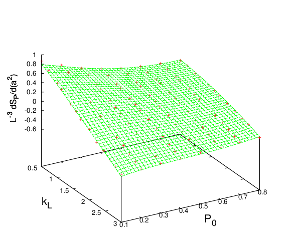
As in the strong coupling case, we choose to investigate the derivatives of along paths of the form (28), i.e. plane waves of fixed wavenumber and varying amplitude on a constant background. The method is the same as outlined in section III, but the result is different. At , it was found that was linear in , and independent of . That is not the case at . What happens in this case is shown in Fig. 9, where we display plotted against the magnitude of lattice momentum at fixed values of and . It can be seen that the -dependence of the data in Fig. 9(a), at , is consistent with linear, while the -dependence in Fig. 9(b), at , seems to be quadratic. This can be seen from fits to in the former case, and to in the latter. This suggests a possible interpolating form
| (55) |
whose -dependence would vary continuously from linear, as , to quadratic, for . Fig. 10 is the same plot as Fig. 9(a), except that data obtained on both an lattice and a volume are displayed together, and both sets of data points appear to have the same dependence. This is, of course, evidence of the insensitivity of our results to the spatial volume.


If (55) is correct, then it ought to be consistent with the potential (49). This means that can be, at most, quadratic in , so let us write
| (56) |
The constants shown are subject to three constraints by the potential, so if we insist on the potential (49) there are really only two independent constants. In order to derive those constraints, consider a very large lattice volume , such that can be made very small compared to , but still non-zero, and we assume that do not vary much with (we have already seen evidence of this fact in Fig. 6). Then the kinetic term is negligible compared to the potential term, and along the trajectory (28), taking account of the spatial average , we have
| (57) |
Comparison with (56) in the limit calls for identifying
| (58) |
Figure 11 show a best fit of the data to the form (56), with the best fit constants given in Table 3. This is hardly a perfect fit through the data points, given the value of the reduced . Still, except at very low , the fitting function gives a reasonable account of the dependence of the data on and . Table 4 is a test of constraints, listing three combinations of constants which, according to the identities (58), should vanish. It is seen that the second and third combinations in the table are consistent with zero, and the first combination is very nearly so.44 4 All fits, and error estimates on fitting constants, are made using the GNUPLOT software.
VII Towards the full action
The interesting question, of course, is what is the full action which gives rise to the variation (56) along the path, with the given potential (49). We begin by noting that, with the constants shown in Tables 1 and 3, the action
| (59) | |||||
where is the kinetic term
| (60) |
and
| (61) | |||||
gives the known results for the potential (49) and for the variation of with (56) along the paths of plane wave deformations (28). The operator is the usual lattice Laplacian operator, and has the spectral representation
| (62) |
where is shorthand for the sum over lattice wave vectors with components , and lattice momentum has been defined previously in (31). The ket vectors correspond to normalized plane wave states.
For the paths (28), set , and compute the resulting action on such configurations up to leading order in . Using the spectral representation for the operator , a short calculation gives, up to ,
| (63) |
Applying the identities (58), which are reasonably well satisfied by the data, this becomes
| (64) |
So we find that for constant configurations (), the action is simply the known potential, i.e. , while the path derivative is
| (65) |
in complete agreement with (56).
Denote by and the lattice average value and mean square deviation, respectively, of a given Polyakov line configuration. It is clear that for the paths (28) considered so far, . One further generalization, which will not affect agreement with the data so far, is to allow the kinetic term to also depend on , i.e. 55 5 A generalization of (59) which does not work is the replacement of by in (59) and (61). This leads to additional contributions to which spoil the agreement with (65).
| (66) |
It is not hard to see that the O() contribution that would arise from the -dependence of the square root terms also selects, at this order, the constant -independent part of and . In that case , and this contribution to the O() part of the kinetic term vanishes.
In order to investigate the possibility of a -dependence a little further, let us consider trajectories consisting of plane waves, of varying amplitude , with , i.e.
| (67) |
and study the derivative evaluated at . To compute this derivative by the relative weights approach, we construct a set of configurations
| (68) |
and proceed as before. The conjectured action is
| (69) | |||||
whose path derivative is 66 6 The numbers multiplying are the lattice averages of respectively. These numbers are almost independent of the wavenumber on finite lattices, so long as , and converge rapidly to the infinite volume limit as lattice volume increases.
| (70) | |||||

Taking and as given in Tables 1 and 4, there is only one free constant left to fit the data, and the best fit, shown in Fig. 12, is obtained at . Once again, this plot should not be interpreted as a perfect fit through the data points within errorbars, given that reduced . On the other hand, with only one fitting constant, the expression (70) does seem to give a quite reasonable account of the dependence of the data on and , despite the highly non-local expression introduced into the kinetic term.
VIII Conclusions
I have presented a method for computing derivatives of the effective Polyakov line action along any given path through field configuration space, parametrized by the variable . The technique is easily implemented in a lattice Monte Carlo code by simply replacing updates of timelike links, on a single timeslice, by a Metropolis step which updates that set of links simultaneously, and the potential part of the effective Polyakov line action can be readily determined, for any given lattice coupling, temperature, and set of matter fields, up to an irrelevant constant. It is also possible to determine, from the derivatives, the action along any given trajectory in field configuration space.
The method has been applied here to SU(2) lattice gauge theory, both without and with a scalar matter field. At a strong coupling () and finite temperature, the method easily determines the effective Polyakov line action, which we have checked against the known result derived from a strong-coupling expansion. At a weaker coupling ( on a lattice), where the Polyakov line action is not known, it has been shown that, up to a constant, the potential term has the form
| (71) |
with coefficients given in Table 1. The center-symmetric but non-analytic cubic term comes as a surprise; to the best of my knowledge such a term has not been anticipated in previous studies. It would be interesting to study the evolution of the above potential as and vary. Addition of a scalar matter field in the underlying lattice gauge theory introduces a center symmetry breaking term into the potential which is linear in , with a coefficient reported in section V.
Data has also been obtained from small plane-wave deformations around a constant Polyakov line background (Section VI), and for Polyakov lines proportional to a plane waves with variable amplitude (Section VII). It was found that the action (69) is consistent with the results that have been found so far, and at this point we may conjecture that (69) approximates the desired full Polyakov line action. Of course, the kinetic term in could easily have a more complicated form than what is suggested in (69), and therefore this conjecture needs to be tested on more complicated, non-plane wave configurations. Those tests, and the extension to the SU(3) group, would be the obvious next steps in the approach introduced here.
Acknowledgements.
It is a pleasure to thank Kim Splittorff for many helpful suggestions. This research is supported in part by the U.S. Department of Energy under Grant No. DE-FG03-92ER40711.References
- [1] M. Fromm, J. Langelage, S. Lottini, and O. Philipsen, JHEP 1201, 042 (2012), arXiv:1111.4953.
- [2] Y. D. Mercado and C. Gattringer, (2012), arXiv:1204.6074.
- [3] G. Aarts and F. A. James, JHEP 1201, 118 (2012), arXiv:1112.4655.
- [4] J. Greensite and K. Splittorff, (2012), arXiv:1206.1159.
- [5] C. Wozar, T. Kaestner, A. Wipf, and T. Heinzl, Phys.Rev. D76, 085004 (2007), arXiv:0704.2570.
- [6] T. Heinzl, T. Kaestner, and A. Wipf, Phys.Rev. D72, 065005 (2005), arXiv:hep-lat/0502013.
- [7] A. Gocksch and M. Ogilvie, Phys.Rev.Lett. 54, 1772 (1985).
- [8] M. Ogilvie, Phys.Rev.Lett. 52, 1369 (1984).
- [9] J. Greensite and J. Iwasaki, Phys. Lett. B223, 207 (1989).
- [10] J. Greensite, H. Matevosyan, Š. Olejník, M. Quandt, H. Reinhardt, and A.P. Szczepaniak, Phys.Rev. D83, 114509 (2011), arXiv:1102.3941.
- [11] E. H. Fradkin and S. H. Shenker, Phys.Rev. D19, 3682 (1979).
- [12] K. Osterwalder and E. Seiler, Annals Phys. 110, 440 (1978).
- [13] C. Bonati, G. Cossu, M. D’Elia, and A. Di Giacomo, Nucl.Phys. B828, 390 (2010), arXiv:0911.1721.