跳到论文正文
W Papers独立论文阅读器 arXiv:1209.5513 论文正文 计算阅读时间 · 0%
引用这篇论文根据当前论文元数据生成,正式投稿前建议核对。


License: arXiv.org perpetual non-exclusive license
arXiv:1209.5513v2 [cs.IT] 26 Sep 2012

On Capacity of Large-Scale MIMO Multiple Access Channels with
Distributed Sets of Correlated Antennas

The work of J. Zhang, S. Jin, and X. Q. Gao was supported by the National Natural Science Foundation of China under Grants 60902009, 61222102 and 61201171, the Natural Science Foundation of Jiangsu Province under Grants BK2012021, and the Supporting Program for New Century Excellent Talents in University (NCET-11-0090). The work of C.-K. Wen was supported by the National Science Council, Taiwan, under grant NSC100-2221-E-110-052-MY3.
Jun Zhang Note: J. Zhang, S. Jin, and X. Q. Gao are with the National Mobile Communications Research Laboratory, Southeast University, Nanjing 210096, China, Email: {mtzhangjun, jinshi, xqgao}@seu.edu.cn.    Chao-Kai Wen Note: Institute of Communications Engineering, National Sun Yat-sen University, Taiwan. Email: ckwen@ieee.org.    Shi Jin    Xiqi Gao    Kai-Kit Wong Note: Department of Electronic and Electrical Engineering, University College London, UK, Email: k.wong@ee.ucl.ac.uk.
Abstract

In this paper, a deterministic equivalent of ergodic sum rate and an algorithm for evaluating the capacity-achieving input covariance matrices for the uplink large-scale multiple-input multiple-output (MIMO) antenna channels are proposed. We consider a large-scale MIMO system consisting of multiple users and one base station with several distributed antenna sets. Each link between a user and an antenna set forms a two-sided spatially correlated MIMO channel with line-of-sight (LOS) components. Our derivations are based on novel techniques from large dimensional random matrix theory (RMT) under the assumption that the numbers of antennas at the terminals approach to infinity with a fixed ratio. The deterministic equivalent results (the deterministic equivalent of ergodic sum rate and the capacity-achieving input covariance matrices) are easy to compute and shown to be accurate for realistic system dimensions. In addition, they are shown to be invariant to several types of fading distribution.

Index Terms—Deterministic equivalent, large dimensional RMT, large-scale MIMO, Stieltjes transform.

1 Introduction

To achieve higher rates, much efforts have been put to improving the spectral efficiency and data throughput of wireless communication systems. The multi-antenna technology is one key technology for wireless communication and is envisaged to be adopted ubiquitously. With the number of antennas at the base stations (BSs) and user equipments (UEs) being increased, communications systems will have better rate and link reliability [1, 2]. However, the actual achievable spectral efficiency could be greatly compromised by interference arising from simultaneous communications in neighboring areas.

A promising solution to interference management is the large-scale multiple-input multiple-output (MIMO) technology, e.g., [3, 4, 5, 6, 7]. Figure 1 illustrates a possible scenario where the antenna array of a BS is composed of multiple geographically distributed low-power antenna sets, installed onto a ring of high-speed fibre-bus, and this BS is communicating with several multi-antenna UEs. The large-scale MIMO setting is beneficial not only in terms of communication performances (such as better coverage and efficient radio resource utilization) but also in terms of energy-saving.11 1 Using the setting, the number of BS can be greatly reduced. Note that the energy consumption for air conditioning for each BS is consuming up to 20,000 kWh each year on average which is sometimes higher than other equipments in a BS [8]. In this complex system model, a number of practical factors such as correlation effects and line-of-sight (LOS) components need to be included, which occur due to the space limitation of UEs and the densification of the antenna arrays resulting in a visible propagation path from the UEs, respectively. For typical systems of tens of distributed antenna sets and hundreds of UEs, even computer simulations become challenging [9], which makes performance analysis of such large-scale MIMO systems an important and a new subject of research.

Refer to caption
Figure 1: A vision for a possible large-scale MIMO system.

When a system is large, exact performance analysis is no longer suitable because an exact analytical expression would be too complex to appreciate. Hence, alternatives have emerged and the large dimensional random matrix theory (RMT) [10, 11, 12, 13, 14, 15, 16, 17, 18, 19, 6] provides a powerful tool in dealing with large-scale MIMO systems. Utilizing the large dimensional RMT, this paper aims to derive information-theoretic results of the large-scale MIMO systems. In particular, our focus is on the uplink large-scale MIMO systems consisting of KK UEs and a BS with LL distributed sets of multiple antennas. Let nkn_{k} and NlN_{l} denote, respectively, the numbers of antennas at the kk-th UE and the ll-th antenna set of the BS receiver. The channel between the kk-th UE and the ll-th antenna set is modeled as the Nl×nkN_{l}\times n_{k} complex matrix 𝐇l,k=𝐑l,k12​𝐗l,k​𝐓l,k12+𝐇¯l,k{\bf H}_{l,k}={\bf R}_{l,k}^{\frac{1}{2}}{\bf X}_{l,k}{\bf T}_{l,k}^{\frac{1}{2}}+{\bar{{\bf H}}}_{l,k}, where 𝐗l,k{\bf X}_{l,k}’s are statistically independent random matrices of independent and identically distributed (i.i.d.) entries (but not necessary Gaussian22 2 Despite the Rayleigh or Rician distribution being the most popular distributions for small-scale amplitude fading, there are other classes of fading distributions which serve as better models under certain circumstances [20, 21].), 𝐇¯l,k{\bar{{\bf H}}}_{l,k} is a deterministic matrix reflecting the LOS components of the channel, and 𝐑l,k{\bf R}_{l,k} and 𝐓l,k{\bf T}_{l,k}, respectively, characterize the spatial correlation structures at the receiver and transmitter sides separatively. Since the signals from multiple antenna sets are collected into a BS, the corresponding channel matrix of UE kk can be expressed as 𝐇k≜[𝐇1,kT⋯𝐇L,kT]T{\bf H}_{k}\triangleq[{\bf H}_{1,k}^{T}\cdots{\bf H}_{L,k}^{T}]^{T}. An important objective of this study is to obtain a deterministic equivalent of the ergodic sum rate for the distributed uplink MIMO channel ∑k=1K𝐇k​𝐇kH\sum_{k=1}^{K}{\bf H}_{k}{\bf H}_{k}^{H} so that the system sum rate can be efficiently and accurately computed.

Although there have been quite many such results on MIMO capacity analysis utilizing large dimensional RMT [10, 12, 13, 14, 15, 16], the general model studied in this paper has not been addressed. To appreciate the objective of this paper, it is important to understand the limitations of the existing results. First, previous works in the large-scale MIMO systems usually assumed nk=1n_{k}=1 and Nl=1N_{l}=1 for all k,lk,l. That is, the UEs have only one antenna each and the BS is equipped with completely distributed antennas (i.e., one antenna in each antenna set). The elements of this channel matrix merely reflect the path loss differences between the links. Regarding the channel model (the channel with a variance profile), the most relevant work is [12] (or [11, Theorem 3.8] without the LOS components). In [12], a deterministic equivalent of the mutual information33 3 Formally, it should be read as the mutual information between the input and output over the channel with a variance profile. In this paper, we often simply refer to it as “the mutual information” if no confusion would occur. was derived based on the Bai-and-Silverstein method [22] (or [17, Chapter 6.2.1]). In fact, the results of [12] can be easily extended to the case with nk≥1n_{k}\geq 1 and Nl≥1N_{l}\geq 1 but those spatial correlation matrices 𝐓l,k{\bf T}_{l,k}’s and 𝐑l,k{\bf R}_{l,k}’s are required to be diagonal.

The deterministic approximations of [12, 11] have found many applications in various system optimization designs such as scheduling [9, 23], training length designs [24], cell planning [25], and many others [17, 11]. This is because the designs based on the deterministic approximations not only can provide an efficient computation method but also give insight into what the optimal strategies look like. However, inheriting from the limitations of [12, 11], these results do not allow the UEs or each antenna set of the BS to be equipped with multiple spatially correlated antennas. Because of the potential applicability of deterministic equivalent results to system designs, there is a strong desire to deriving new deterministic equivalents as those given in [12] for the general model of our interest. However, even for an extension to the one-sided spatially correlated case, there will be several obstacles when one intends to get the deterministic equivalent of mutual information by using the Bai-and-Silverstein method and alike.44 4 If 𝐇¯l,k=𝟎​∀l,k{\bar{{\bf H}}}_{l,k}={\bf 0}~\forall l,k, a partial generalization is possible by the Bai-and-Silverstein method. Specifically, with minor modifications for the case in [26, 16], the asymptotic mutual information can be obtained for the case that 𝐑l,k{\bf R}_{l,k}’s were permitted to be nonnegative definite, while 𝐇¯l,k=𝟎{\bar{{\bf H}}}_{l,k}={\bf 0} and 𝐓l,k{\bf T}_{l,k}’s are diagonal. If 𝐓l,k{\bf T}_{l,k}’s are generally nonnegative definite, difficulties arise.

To date, there are only very few results dealing with random matrix models where the entries are correlated across both rows and columns. Most studies only considered random matrices with independent complex Gaussian random variables and used the fact that the correlated Gaussian random matrix can be transformed to an uncorrelated one with non-identically distributed entries without changing the concerned objects (e.g., the eigenvalue distribution and the mutual information). For convenience, we will refer to this transformation as the decorrelation procedure. Because of the assumption of Gaussianity the entries are in fact uncorrelated, and so the Bai-and-Silverstein method can be used. For the latest results using this trick, refer to, e.g., [16]. Unfortunately, the channel model of our interest (i.e., 𝐇k{\bf H}_{k}) cannot be transformed to a Gaussian random matrix with uncorrelated columns even if 𝐗l,k{\bf X}_{l,k}’s are assumed to be Gaussian. For this to be possible, it would require that 𝐓1,k,…,𝐓L,k{\bf T}_{1,k},\dots,{\bf T}_{L,k} be simultaneously unitarily diagonalizable for every kk. Clearly, this restriction in the model does not permit UEs to have multiple spatially correlated antennas, which is unrealistic and greatly limits the significance of the model.

If the entries of the random matrices are Gaussian, then an alternative method, known as the Gaussian method [27] (the integration by part formula and Poincaré-Nash inequality), is much more useful. In this context, Hachem et al. [13, 15] have succeeded in obtaining the deterministic equivalent of mutual information for Kronecker (or separately) correlated Rayleigh and Rician MIMO channels. Compared to the Bai-and-Silverstein method, the Gaussian method is only suited to random matrices with Gaussian entries. However, one may extend the results obtained for matrices with Gaussian entries to any random matrices with independent entries following two recent developments, the Lindeberg principle [28] and the interpolation trick [29]. For the latest results, see, e.g., [19], where the Lindeberg principle is applied.

Early analyses using the Gaussian method were only for the typical Kronecker MIMO channel [13, 15].55 5 In this paper, the typical Kronecker MIMO channel means that K=L=1K=L=1. In that case, the correlated Gaussian random matrix was transformed into an uncorrelated one, and the decorrelation procedure was employed. As such, the Gaussian method was merely an alternative tool to study large dimensional random matrices. Its superiority in dealing with random matrices with correlated pattern is largely unexplored until most recently, Dupuy and Loubaton in [18] derived the deterministic equivalent of average mutual information for a frequency selective MIMO channel, in which the decorrelation procedure could not be applied. We believe that the Gaussian method can be useful to treat other random matrices with involved correlation. With the aid of the Lindeberg principle, one may further extend the results obtained for matrices with Gaussian entries to any random matrices. Following this approach, this paper combines the two techniques to get the deterministic equivalents for the concerned channel model.

In particular, we first use the Gaussian method to derive the deterministic equivalent of ergodic sum rate for the large-scale MIMO multiple access channel (MAC) when 𝐗l,k{\bf X}_{l,k}’s are Gaussian distributed. Our results are much more general and can cope with several complex applications. As a special case, this contribution complements the results of [18] by extending the analysis to the case with LOS components. This extension is non-trivial.66 6 Using the Gaussian tools, the asymptotic mutual information expressions for Rayleigh fading Kronecker MIMO channels were first proved by [13]. Two years later, the authors in the same group generalized the results to Rician fading channels [15]. This in some ways reflects the difficulty of such extension even for the typical Kronecker MIMO channel. Next, by the generalized Lindeberg principle [28, 30], we generalize the deterministic equivalent for random matrices with Gaussian entries to those with non-Gaussian entries. Simulation results reveal that even for systems with realistic system dimensions, the deterministic approximation of ergodic sum rate provides reliable estimates to those obtained by Monte-Carlo simulations. Then, we apply the approximation to design the input covariances that tend to maximize the ergodic sum rate of the large-scale MIMO MAC, and provide an iterative water-filling optimization algorithm when only the statistical CSI at the transmitter (precisely, 𝐓l,k{\bf T}_{l,k}’s, 𝐑l,k{\bf R}_{l,k}’s, and 𝐇¯l,k{\bar{{\bf H}}}_{l,k}’s) is available. Finally, we conduct several simulations to confirm the comparability between results by our approach and those by the true (but time-consuming) optimization procedure under several types of fading distribution.

Notations—We use uppercase and lowercase boldface letters to denote matrices and vectors, respectively. 𝐈N{\bf{I}}_{N} denotes an N×NN\times N identity matrix while an all-zero matrix is denoted by 𝟎{\bf{0}}, and an all-one matrix is denoted by 𝟏{\bf{1}}. The matrix inequality ⪰\succeq shows the positive semi-definiteness. The superscripts (⋅)H(\cdot)^{H}, (⋅)T(\cdot)^{T}, and (⋅)∗(\cdot)^{*} represent the conjugate-transpose, transpose, and conjugate operations, respectively. Also, we use 𝖤​{⋅}{\sf E}\{\cdot\} to denote expectation with respect to all random variables within the brackets; log⁡(⋅)\log(\cdot) is the natural logarithm; ρ⁡(⋅)\rho(\cdot) denotes the spectral radius (i.e., the largest absolute value of the eigenvalues) of a matrix. ∥⋅∥\|\cdot\| represents the Euclidean norm of an input vector or the spectral norm of an input matrix, while ∥⋅∥F\|\cdot\|_{\rm F} denotes the Frobenius norm of a matrix, and |||⋅|||∞\mbox{$\left|\!\left|\!\left|\,\cdot\,\right|\!\right|\!\right|$}_{\infty} represents the maximum row sum matrix norm. The complex number field is denoted by ℂ\mathbb{C}. For any matrix 𝐀∈ℂN×n{\bf A}\in\mathbb{C}^{N\times n}, we use [𝐀]l​k[{\bf A}]_{lk}, [𝐀]l,k[{\bf A}]_{l,k} or Ak​lA_{kl} to denote the (ll,kk)-th entry, and aka_{k} denotes the kk-th entry of the column vector 𝐚\bf{a}. The operators (⋅)12(\cdot)^{\frac{1}{2}}, (⋅)−1(\cdot)^{-1}, 𝗍𝗋⁡(⋅){{\sf tr}}(\cdot) and det(⋅)\det(\cdot) represent the matrix principal square root, inverse, trace and determinant, respectively. In addition, 𝖽𝗂𝖺𝗀⁡(𝐱){\sf diag}(\bf{x}) denotes a diagonal matrix with an input vector 𝐱\bf{x} representing its diagonal elements.

2 Channel Model and Problem Statement

2.1 Uplink Large MIMO

As shown in Figure 1, we consider the large-scale MIMO MAC with KK UEs, labeled as 𝖴𝖤1,…,𝖴𝖤K{\sf UE}_{1},\dots,{\sf UE}_{K}, which are equipped with n1,…,nKn_{1},\dots,n_{K} antennas, respectively. The KK UEs transmit simultaneously to a central coordinator with LL distributed antenna sets, labeled as 𝖡𝖲1,…,𝖡𝖲L{\sf BS}_{1},\dots,{\sf BS}_{L}, which are equipped with N1,…,NLN_{1},\dots,N_{L} antennas, respectively. In this paper, we use the Kronecker model to characterize the spatial correlation of the MIMO channel for each MIMO link so that the correlation at an antenna set and a UE is modeled separately, as in [31]. Specifically, the channel from 𝖴𝖤k{\sf UE}_{k} to 𝖡𝖲l{\sf BS}_{l}, 𝐇l,k∈ℂNl×nk{\bf H}_{l,k}\in{\mathbb{C}}^{N_{l}\times n_{k}}, can be written as

𝐇l,k=𝐇~l,k+𝐇¯l,k≡𝐑l,k12​𝐗l,k​𝐓l,k12+𝐇¯l,k,{\bf H}_{l,k}={\tilde{{\bf H}}}_{l,k}+{\bar{{\bf H}}}_{l,k}\equiv{\bf R}_{l,k}^{\frac{1}{2}}{\bf X}_{l,k}{\bf T}_{l,k}^{\frac{1}{2}}+{\bar{{\bf H}}}_{l,k}, (1)

where 𝐑l,k∈ℂNl×Nl{\bf R}_{l,k}\in{\mathbb{C}}^{N_{l}\times N_{l}} and 𝐓l,k∈ℂnk×nk{\bf T}_{l,k}\in{\mathbb{C}}^{n_{k}\times n_{k}} are deterministic nonnegative definite matrices, characterizing the spatial correlation of the received signals across the antenna elements of 𝖡𝖲l{\sf BS}_{l} and that of the transmitted signals across the antenna elements of 𝖴𝖤k{\sf UE}_{k}, respectively; 𝐗l,k≡[1nk​Xi​j(l,k)]∈ℂNl×nk{\bf X}_{l,k}\equiv[\frac{1}{\sqrt{n_{k}}}X_{ij}^{(l,k)}]\in{\mathbb{C}}^{N_{l}\times n_{k}} consists of the random components of the channel in which the elements are i.i.d. complex random variables with zero mean and unit variance; and 𝐇¯l,k∈ℂNl×nk{\bar{{\bf H}}}_{l,k}\in{\mathbb{C}}^{N_{l}\times n_{k}} is a deterministic matrix corresponding to the channel LOS.

With the channel given above, we define the Rician factor between 𝖴𝖤k{\sf UE}_{k} and 𝖡𝖲l{\sf BS}_{l} as

κl,k=‖𝐇¯l,k‖F2𝖤⁡{‖𝐇~l,k‖F2}.\kappa_{l,k}=\frac{\|{\bar{{\bf H}}}_{l,k}\|_{\rm F}^{2}}{{\sf E}{\{\|{\tilde{{\bf H}}}_{l,k}\|_{\rm F}^{2}\}}}. (2)

We also denote the distance-dependent pathloss of the (l,k)(l,k)-th pair by gl,k=𝖤⁡{‖𝐇l,k‖F2}/Nlg_{l,k}={\sf E}{\left\{\|{\bf H}_{l,k}\|_{\rm F}^{2}\right\}}/N_{l} given by

𝖤⁡{‖𝐇l,k‖F2}=1nk​𝗍𝗋​(𝐑l,k)​𝗍𝗋​(𝐓l,k)+𝗍𝗋⁡(𝐇¯l,k​𝐇¯l,kH).{\sf E}{\left\{\|{\bf H}_{l,k}\|_{\rm F}^{2}\right\}}=\frac{1}{n_{k}}{\sf tr}{\left({\bf R}_{l,k}\right)}{\sf tr}{\left({\bf T}_{l,k}\right)}+{\sf tr}{\left({\bar{{\bf H}}}_{l,k}{\bar{{\bf H}}}_{l,k}^{H}\right)}. (3)

Following the standard conventions [14], 𝐑l,k{\bf R}_{l,k}, 𝐓l,k{\bf T}_{l,k}, and 𝐇¯l,k{\bar{{\bf H}}}_{l,k} are normalized such that

{𝗍𝗋⁡(𝐑l,k)=1κl,k+1​gl,k​Nl,𝗍𝗋⁡(𝐓l,k)=nk,𝗍𝗋⁡(𝐇¯l,k​𝐇¯l,kH)=κl,kκl,k+1​gl,k​Nl.\left\{\begin{aligned} {\sf tr}{({\bf R}_{l,k})}&=\frac{1}{\kappa_{l,k}+1}g_{l,k}N_{l},\\ {\sf tr}{({\bf T}_{l,k})}&=n_{k},\\ {\sf tr}{\left({\bar{{\bf H}}}_{l,k}{\bar{{\bf H}}}_{l,k}^{H}\right)}&=\frac{\kappa_{l,k}}{\kappa_{l,k}+1}g_{l,k}N_{l}.\end{aligned}\right. (4)

It is noted that κl,k\kappa_{l,k} and gl,kg_{l,k} are independent from the matrix dimensions. Therefore, the normalization is valid for all possible correlation patterns and imposes no restriction on practical applications. Although for convenience purpose we will simply set the same noise level (i.e., σ2\sigma^{2}) at all the receivers, it imposes no restriction since one can adjust gl,kg_{l,k} to get an arbitrary signal-to-noise ratio (SNR) of the (l,k)(l,k)-th pair. In addition, the setting implies that the LOS components of some link pairs are allowed to be absent.

2.2 Problem Formulation

The sum rate has been a key metric for performance analysis of a MAC. We begin with the sum rate formulation of the large-scale MIMO system and then explain its relation to RMT. For ease of exposition, we define N≜∑l=1LNlN\triangleq\sum_{l=1}^{L}N_{l}, n≜∑k=1Knkn\triangleq\sum_{k=1}^{K}n_{k}, 𝐇k≜[𝐇1,kT⋯𝐇L,kT]T∈ℂN×nk{\bf H}_{k}\triangleq\left[{\bf H}_{1,k}^{T}\cdots{\bf H}_{L,k}^{T}\right]^{T}\in{\mathbb{C}}^{N\times n_{k}}, 𝐇¯k≜[𝐇¯1,kT⋯𝐇¯L,kT]T∈ℂN×nk{\bar{{\bf H}}}_{k}\triangleq\left[{\bar{{\bf H}}}_{1,k}^{T}\cdots{\bar{{\bf H}}}_{L,k}^{T}\right]^{T}\in{\mathbb{C}}^{N\times n_{k}}, 𝐇≜[𝐇1⋯𝐇K]∈ℂN×n{\bf H}\triangleq\left[{\bf H}_{1}\cdots{\bf H}_{K}\right]\in{\mathbb{C}}^{N\times n}, and 𝐇¯≜[𝐇¯1⋯𝐇¯K]∈ℂN×n{\bar{{\bf H}}}\triangleq\left[{\bar{{\bf H}}}_{1}\cdots{\bar{{\bf H}}}_{K}\right]\in{\mathbb{C}}^{N\times n}. The channel 𝐇k{\bf H}_{k} represents the joint channel between 𝖴𝖤k{\sf UE}_{k} and the LL distributed antenna sets interconnected at the BS. Then, the ergodic sum rate of the MIMO MAC can be expressed as [32]

𝒱𝐁N(σ2)≡1N𝖤{logdet(𝐈N+1σ2𝐁N)}{\mathcal{V}}_{{\bf B}_{N}}(\sigma^{2})\equiv\frac{1}{N}{\sf E}\left\{\log\det\left({\bf I}_{N}+\frac{1}{\sigma^{2}}{\bf B}_{N}\right)\right\} (5)

where σ2\sigma^{2} is the noise variance at the receivers and

𝐁N≜∑k=1K𝐇k​𝐇kH∈ℂN×N.{\bf B}_{N}\triangleq\sum_{k=1}^{K}{\bf H}_{k}{\bf H}_{k}^{H}~\in{\mathbb{C}}^{N\times N}. (6)

Specifically, 𝒱𝐁N​(σ2){\mathcal{V}}_{{\bf B}_{N}}(\sigma^{2}) provides a performance metric regarding the total number of nats (or bits if in base 2 of logarithm) per antenna that can be transmitted reliably over the channel matrices {𝐇k}k=1,…,K\{{\bf H}_{k}\}_{k=1,\dots,K}.

The derivative of 𝒱𝐁N​(σ2){\mathcal{V}}_{{\bf B}_{N}}(\sigma^{2}) with respect to σ2\sigma^{2} is given by

∂𝒱𝐁N​(σ2)∂σ2=1N​𝖤​{𝗍𝗋⁡[(𝐈N+1σ2​𝐁N)−1]}−1σ2.\frac{\partial{\mathcal{V}}_{{\bf B}_{N}}(\sigma^{2})}{\partial\sigma^{2}}=\frac{1}{N}{\sf E}\left\{{\sf tr}\left[\left({\bf I}_{N}+\frac{1}{\sigma^{2}}{\bf B}_{N}\right)^{-1}\right]\right\}-\frac{1}{\sigma^{2}}. (7)

By Fubini’s theorem, we have [12, page 891]

𝒱𝐁N​(σ2)=∫σ2∞(1ω−𝖤⁡{m𝐁N​(ω)})​𝑑ω,{\mathcal{V}}_{{\bf B}_{N}}(\sigma^{2})=\int_{\sigma^{2}}^{\infty}\left(\frac{1}{\omega}-{\sf E}\{m_{{\bf B}_{N}}(\omega)\}\right)d\omega, (8)

where

m𝐁N​(ω)≜1N​𝗍𝗋​(𝐁N+ω​𝐈N)−1.m_{{\bf B}_{N}}(\omega)\triangleq\frac{1}{N}{\sf tr}\left({\bf B}_{N}+\omega{\bf I}_{N}\right)^{-1}. (9)

In RMT, m𝐁Nm_{{\bf B}_{N}} is referred to as the Stieltjes transform of 𝐁N{\bf B}_{N} at point −ω-\omega, which provides a convenient tool to study the behavior of large dimensional random matrices. The relationship by which the mutual information is expressed as a functional of the Stieltjes transform is called the Shannon transform [11, Section 2.2.3].

In this paper, we are interested in understanding the ergodic sum capacity of the MIMO MAC by using large dimensional RMT. In particular, we consider that LL, KK are fixed but N1,…,NL,n1,…,nKN_{1},\dots,N_{L},n_{1},\dots,n_{K} all go to infinity with ratios {βl,k(N)≡Nlnk}\{\beta_{l,k}(N)\equiv\frac{N_{l}}{n_{k}}\} such that

0<min⁡lim infNl,k⁡βl,k​(N)<max⁡lim supNl,k⁡βl,k​(N)<∞.0<\min_{l,k}\,\liminf_{N}\beta_{l,k}(N)<\max_{l,k}\,\limsup_{N}\beta_{l,k}(N)<\infty. (10)

For convenience, we refer to this large dimensional regime simply as 𝒩→∞\mbox{${\cal N}$}\rightarrow\infty in the sequel. To this end, in the next section, we first find a deterministic matrix-valued function 𝚿⁡(ω)∈ℂN×N{\boldsymbol{\Psi}}(\omega)\in{\mathbb{C}}^{N\times N} (to be done later) such that

𝖤⁡{m𝐁N​(ω)}−1N​𝗍𝗋​(𝚿⁡(ω))→𝒩→∞0​for ​ω∈ℝ+.{\sf E}\left\{m_{{\bf B}_{N}}(\omega)\right\}-\frac{1}{N}{\sf tr}{({\boldsymbol{\Psi}}(\omega))}\xrightarrow{\mbox{${\cal N}$}\rightarrow\infty}0~~\mbox{for }\omega\in{\mathbb{R}}^{+}. (11)

Following [12] (or [17, Definition 6.1]), we refer to 1N​𝗍𝗋​(𝚿⁡(ω))\frac{1}{N}{\sf tr}({\boldsymbol{\Psi}}(\omega)) as the deterministic equivalent of 𝖤​{m𝐁N​(ω)}{\sf E}\left\{m_{{\bf B}_{N}}(\omega)\right\}. To appreciate the contributions of this paper, it is worth emphasizing that 𝐇k{\bf H}_{k}, in general, cannot be written in the form (1) using the separable correlation model, because different antenna sets have different spatial correlations, and this is the main obstacle of this class of random matrices – otherwise, there are some existing results [10, 11, 12, 13, 14, 15, 16, 18, 19, 6]. Next, using the Shannon transform (8), we will find 𝒱N​(σ2){\mathcal{V}}_{N}(\sigma^{2}) so that 𝖤⁡{𝒱𝐁N​(σ2)}−𝒱N​(σ2)→0{\sf E}\{{\mathcal{V}}_{{\bf B}_{N}}(\sigma^{2})\}-{\mathcal{V}}_{N}(\sigma^{2})\rightarrow 0 as 𝒩→∞\mbox{${\cal N}$}\rightarrow\infty. Finally, we will use 𝒱N​(σ2){\mathcal{V}}_{N}(\sigma^{2}) to obtain the optimal input covariance matrices that maximize the deterministic approximation of the ergodic sum rate.

3 Deterministic Equivalents and Ergodic Capacity

3.1 Deterministic Equivalents

We first state the assumptions imposed in our system model.

Assumption 1

Let 𝐗l,k≡[1nk​Xi​j(l,k)]∈ℂNl×nk{\bf X}_{l,k}\equiv[\frac{1}{\sqrt{n_{k}}}X_{ij}^{(l,k)}]\in\mathbb{C}^{N_{l}\times n_{k}}, where Xi​j(l,k)X_{ij}^{(l,k)}’s are i.i.d. complex random variables with independent real and imaginary parts such that

𝖤⁡{X11(l,k)}=0,and​𝖤​{|X11(l,k)|2}=1,{\sf E}\{X_{11}^{(l,k)}\}=0,~\mbox{and}~{\sf E}\{|X_{11}^{(l,k)}|^{2}\}=1, (12)

and have finite 66-th order moment.

Assumption 2

The family of deterministic matrices {𝐓l,k,𝐑l,k}∀l,k\{{\bf T}_{l,k},{\bf R}_{l,k}\}_{\forall l,k} is nonnegative definite. In addition, the spectral norms of 𝐑l,k{\bf R}_{l,k}, 𝐓l,k{\bf T}_{l,k}, and 𝐇¯l,k​𝐇¯l,kH{\bar{{\bf H}}}_{l,k}{\bar{{\bf H}}}_{l,k}^{H} are bounded by a constant, i.e.,

maxk,l⁡max⁡{‖𝐑l,k‖,‖𝐓l,k‖,‖𝐇¯l,k​𝐇¯l,kH‖}≤Cmax.\max_{k,l}\,\max\{\|{\bf R}_{l,k}\|,\|{\bf T}_{l,k}\|,\|{\bar{{\bf H}}}_{l,k}{\bar{{\bf H}}}_{l,k}^{H}\|\}\leq C_{\rm max}. (13)

To facilitate our expressions, we define the notation ⟨𝐀⟩k\mbox{$\langle{\bf A}\rangle$}_{k} that returns the submatrix of 𝐀{\bf A} obtained by extracting the elements of the rows and columns with indices from ∑i=1k−1ni+1\sum_{i=1}^{k-1}n_{i}+1 to ∑i=1kni\sum_{i=1}^{k}n_{i}. Similarly, the notation ⟨⟨𝐀⟩⟩l\mbox{$\langle\!\langle{\bf A}\rangle\!\rangle$}_{l} returns the submatrix of 𝐀{\bf A} obtained by extracting the elements of the rows and columns with indices from ∑j=1l−1Nj+1\sum_{j=1}^{l-1}N_{j}+1 to ∑j=1lNj\sum_{j=1}^{l}N_{j}. Also, for convenience, in the paper, we often omit ω\omega when writing m𝐁N,𝚿,𝚿~,𝚽,𝚽~,𝚽l,𝚽~k,el,k,e~l,km_{{\bf B}_{N}},{\boldsymbol{\Psi}},{\tilde{{\boldsymbol{\Psi}}}},{\boldsymbol{\Phi}},{\tilde{{\boldsymbol{\Phi}}}},{\boldsymbol{\Phi}}_{l},{\tilde{{\boldsymbol{\Phi}}}}_{k},e_{l,k},{\tilde{e}}_{l,k}, and denote ∑l,k≡∑l=1L∑k=1K\sum_{l,k}\equiv\sum_{l=1}^{L}\sum_{k=1}^{K}.

Theorem 1

Let βl,k=Nlnk\beta_{l,k}=\frac{N_{l}}{n_{k}}. Under Assumption 2, the deterministic system of the L×KL\times K equations

el,k\displaystyle e_{l,k} =1Nl​𝗍𝗋​(𝐑l,k​⟨⟨𝚿⟩⟩l),\displaystyle=\frac{1}{N_{l}}{\sf tr}{\left({\bf R}_{l,k}\mbox{$\langle\!\langle{\boldsymbol{\Psi}}\rangle\!\rangle$}_{l}\right)}, (14a)
e~l,k\displaystyle{\tilde{e}}_{l,k} =1nk​𝗍𝗋​(𝐓l,k​⟨𝚿~⟩k),\displaystyle=\frac{1}{n_{k}}{\sf tr}{\left({\bf T}_{l,k}\mbox{$\langle{\tilde{{\boldsymbol{\Psi}}}}\rangle$}_{k}\right)}, (14b)

for 1≤l≤L1\leq l\leq L and 1≤k≤K1\leq k\leq K, where

𝚿\displaystyle{\boldsymbol{\Psi}} =(𝚽−1+ω​𝐇¯​𝚽~​𝐇¯H)−1,\displaystyle={\left({\boldsymbol{\Phi}}^{-1}+\omega{\bar{{\bf H}}}{\tilde{{\boldsymbol{\Phi}}}}{\bar{{\bf H}}}^{H}\right)^{-1}}, (15a)
𝚿~\displaystyle{\tilde{{\boldsymbol{\Psi}}}} =(𝚽~−1+ω​𝐇¯H​𝚽​𝐇¯)−1,\displaystyle={\left({\tilde{{\boldsymbol{\Phi}}}}^{-1}+\omega{\bar{{\bf H}}}^{H}{\boldsymbol{\Phi}}{\bar{{\bf H}}}\right)^{-1}}, (15b)
𝚽\displaystyle{\boldsymbol{\Phi}} =𝖽𝗂𝖺𝗀⁡(𝚽1,…,𝚽L),\displaystyle={\sf diag}{({\boldsymbol{\Phi}}_{1},\ldots,{\boldsymbol{\Phi}}_{L})}, (15c)
𝚽~\displaystyle{\tilde{{\boldsymbol{\Phi}}}} =𝖽𝗂𝖺𝗀⁡(𝚽~1,…,𝚽~K),\displaystyle={\sf diag}{({\tilde{{\boldsymbol{\Phi}}}}_{1},\ldots,{\tilde{{\boldsymbol{\Phi}}}}_{K})}, (15d)
𝚽l\displaystyle{\boldsymbol{\Phi}}_{l} =(ω​𝐈Nl+ω​∑k=1Ke~l,k​𝐑l,k)−1,\displaystyle=\left(\omega{\bf I}_{N_{l}}+\omega\sum_{k=1}^{K}{{{\tilde{e}}_{l,k}}{\bf R}_{l,k}}\right)^{-1}, (15e)
𝚽~k\displaystyle{\tilde{{\boldsymbol{\Phi}}}}_{k} =(ω​𝐈nk+ω​∑l=1Lβl,k​el,k​𝐓l,k)−1\displaystyle=\left(\omega{\bf I}_{n_{k}}+\omega\sum_{l=1}^{L}{{\beta_{l,k}e_{l,k}}{\bf T}_{l,k}}\right)^{-1} (15f)

have a unique solution for ω∈ℝ+\omega\in{\mathbb{R}}^{+}.

Under Assumptions 1 and 2, as 𝒩→∞\mbox{${\cal N}$}\rightarrow\infty, we then have

𝖤⁡{m𝐁N}−1N​𝗍𝗋​(𝚿)=O⁡(1N),for​ω∈ℝ+.{\sf E}\left\{m_{{\bf B}_{N}}\right\}-\frac{1}{N}{\sf tr}{({\boldsymbol{\Psi}})}=O\left(\frac{1}{\sqrt{N}}\right),~~\mbox{for}~\omega\in{\mathbb{R}}^{+}. (16)

Furthermore, if 𝐗l,k{\bf X}_{l,k}’s are Gaussian, we have

𝖤⁡{m𝐁N}−1N​𝗍𝗋​(𝚿)=O⁡(1N2),for​ω∈ℝ+.{\sf E}\left\{m_{{\bf B}_{N}}\right\}-\frac{1}{N}{\sf tr}{({\boldsymbol{\Psi}})}=O\left(\frac{1}{N^{2}}\right),~~\mbox{for}~\omega\in{\mathbb{R}}^{+}. (17)

Proof: Here, for ease of understanding, we give an outline of the proof. Our strategy is to show that the deterministic equivalent of 𝖤​{m𝐁N}{\sf E}\left\{m_{{\bf B}_{N}}\right\} [i.e. 1N​𝗍𝗋​(𝚿)\frac{1}{N}{\sf tr}{({\boldsymbol{\Psi}})}] can be found for the Gaussian random matrices and then we prove that the result is also applied for the non-Gaussian distributions.

Let ℬN\boldsymbol{\cal B}_{N} be an N×NN\times N matrix obtained from 𝐁N{\bf B}_{N} in (6) with all 𝐗l,k{\bf X}_{l,k}’s replaced by 𝒳l,k\boldsymbol{\cal X}_{l,k}’s, where 𝒳l,k\boldsymbol{\cal X}_{l,k}’s are matrices with entries being independent standard Gaussian. Using the Gaussian method [27] (the integration by part formula and Poincaré-Nash inequality), we can show that the error term 𝖤​{mℬN}−1N​𝗍𝗋​(𝚿){\sf E}\{m_{\boldsymbol{\cal B}_{N}}\}-\frac{1}{N}{\sf tr}{\left({\boldsymbol{\Psi}}\right)} is of order O⁡(1N2)O\left(\frac{1}{N^{2}}\right). The detailed derivation is given in Appendix A.

Next, applying the Lindeberg principle [30, Theorem 2], we prove that 𝖤⁡{m𝐁N}−𝖤⁡{mℬN}=O⁡(1N){\sf E}\{m_{{\bf B}_{N}}\}-{\sf E}\{m_{\boldsymbol{\cal B}_{N}}\}=O\left(\frac{1}{\sqrt{N}}\right). The detailed derivation using the Lindeberg principle is provided in Appendix B. Together with the result for the Gaussian case, the proof of (16) can be accomplished by noting that

𝖤⁡{m𝐁N}−1N​𝗍𝗋​(𝚿)=(𝖤⁡{m𝐁N}−𝖤⁡{mℬN})⏟=O⁡(1N)+(𝖤⁡{mℬN}−1N​𝗍𝗋​(𝚿))⏟=O⁡(1N2).{\sf E}\left\{m_{{\bf B}_{N}}\right\}-\frac{1}{N}{\sf tr}\left({\boldsymbol{\Psi}}\right)=\underbrace{\Big({\sf E}\left\{m_{{\bf B}_{N}}\right\}-{\sf E}\left\{m_{\boldsymbol{\cal B}_{N}}\right\}\Big)}_{=O\left(\frac{1}{\sqrt{N}}\right)}+\underbrace{\Big({\sf E}\left\{m_{\boldsymbol{\cal B}_{N}}\right\}-\frac{1}{N}{\sf tr}\left({\boldsymbol{\Psi}}\right)\Big)}_{=O\left(\frac{1}{N^{2}}\right)}.

Finally, we consider the existence and uniqueness of the solution to (14) in Appendix C.  □\square

Remark 1

If Xi​j(l,k)X_{ij}^{(l,k)}’s are Gaussian, the assumption that Xi​j(l,k)X_{ij}^{(l,k)}’s have finite 66-th order moment is naturally satisfied. When the amplitudes of the channel fading coefficients follow the Nakagami and log-normal distributions, Theorem 1 is applicable since these distributions have finite 66-th order moment. In Appendix B, the proof of 𝖤⁡{m𝐁N}−1N​𝗍𝗋​(𝚿)=O⁡(1N){\sf E}\left\{m_{{\bf B}_{N}}\right\}-\frac{1}{N}{\sf tr}{({\boldsymbol{\Psi}})}=O\left(\frac{1}{\sqrt{N}}\right) was given under the assumption that Xi​j(l,k)X_{ij}^{(l,k)}’s have finite 66-th order moment. In fact, with additional arguments, the more general case can be obtained. Specifically, if Xi​j(l,k)X_{ij}^{(l,k)}’s have only finite second moment, we can prove that 𝖤⁡{m𝐁N​(ω)}−1N​𝗍𝗋​(𝚿⁡(ω))=O⁡(εn){\sf E}\left\{m_{{\bf B}_{N}}(\omega)\right\}-\frac{1}{N}{\sf tr}{({\boldsymbol{\Psi}}(\omega))}=O\left(\varepsilon_{n}\right), where εn\varepsilon_{n} is a positive sequence converging to zero. However, it should be noted that with the finite 66-th order moment assumption, the proof of 𝖤⁡{m𝐁N}−1N​𝗍𝗋​(𝚿)=O⁡(1N){\sf E}\left\{m_{{\bf B}_{N}}\right\}-\frac{1}{N}{\sf tr}{({\boldsymbol{\Psi}})}=O\left(\frac{1}{\sqrt{N}}\right) is much simpler than the latter general case. The proof of the general case requires some additional truncation, centralization, and rescaling techniques together with some careful derivations as those in [19]. Since these are beyond the scope of this paper, we do not show the detail proof regarding this general case. Interested readers can refer to [19].

Remark 2

Theorem 1 is developed under the asymptotic regime where LL, KK are fixed but {Nl,nk}\{N_{l},n_{k}\}’s all grow to infinity with fixed ratios. For other applications, we might be interested in the cases with fixed {Nl,nk}\{N_{l},n_{k}\}’s while LL and KK grow to infinity. In this case, the entries of 𝐗l,k{\bf X}_{l,k}’s will be normalized by n\sqrt{n} rather than nk\sqrt{n_{k}} and a similar deterministic equivalent result as that of Theorem 1 can be obtained.77 7 Only different in some scalar adjustment.

We then derive a deterministic equivalent of the ergodic sum rate of the large-scale MIMO MAC in the following theorem.

Theorem 2

Assuming that 𝐁N{\bf B}_{N} follows the hypotheses of Theorem 1, as 𝒩→∞\mbox{${\cal N}$}\rightarrow\infty, the Shannon transform of 𝐁N{\bf B}_{N} satisfies

𝖤⁡{𝒱𝐁N​(σ2)}−𝒱N​(σ2)=O⁡(1N),{\sf E}\{{\mathcal{V}}_{{\bf B}_{N}}(\sigma^{2})\}-{\mathcal{V}}_{N}(\sigma^{2})=O\left(\frac{1}{\sqrt{N}}\right), (18)

where

𝒱N​(σ2)\displaystyle{\mathcal{V}}_{N}(\sigma^{2}) =1Nlogdet(𝚿​(σ2)−1σ2)+1N∑k=1Klogdet(𝚽~k​(σ2)−1σ2)−σ2N∑l,kNlel,k(σ2)e~l,k(σ2),\displaystyle=\frac{1}{N}\log\det{\left(\frac{{\boldsymbol{\Psi}}(\sigma^{2})^{-1}}{\sigma^{2}}\right)}+\frac{1}{N}\sum_{k=1}^{K}{{\log\det\left(\frac{{\tilde{{\boldsymbol{\Phi}}}}_{k}(\sigma^{2})^{-1}}{\sigma^{2}}\right)}}-\frac{\sigma^{2}}{N}\sum_{l,k}{N_{l}e_{l,k}(\sigma^{2}){\tilde{e}}_{l,k}(\sigma^{2})}, (19a)
=1Nlogdet(𝚿~​(σ2)−1σ2)+1N∑l=1Llogdet(𝚽l​(σ2)−1σ2)−σ2N∑l,kNlel,k(σ2)e~l,k(σ2).\displaystyle=\frac{1}{N}\log\det{\left(\frac{{\tilde{{\boldsymbol{\Psi}}}}(\sigma^{2})^{-1}}{\sigma^{2}}\right)}+\frac{1}{N}\sum_{l=1}^{L}{{\log\det\left(\frac{{\boldsymbol{\Phi}}_{l}(\sigma^{2})^{-1}}{\sigma^{2}}\right)}}-\frac{\sigma^{2}}{N}\sum_{l,k}{N_{l}e_{l,k}(\sigma^{2}){\tilde{e}}_{l,k}(\sigma^{2})}. (19b)

Furthermore, if 𝐗l,k{\bf X}_{l,k}’s are Gaussian, we have, as 𝒩→∞\mbox{${\cal N}$}\rightarrow\infty,

N⁡(𝖤⁡{𝒱𝐁N​(σ2)}−𝒱N​(σ2))=O⁡(1N).N\left({\sf E}\{{\mathcal{V}}_{{\bf B}_{N}}(\sigma^{2})\}-{\mathcal{V}}_{N}{(\sigma^{2})}\right)=O\left(\frac{1}{N}\right). (20)

Proof: By (16) in Theorem 1 together with the dominated convergence theorem, (18) is obtained. Then, we show that ∫σ2∞(1ω−1N​𝗍𝗋​(𝚿⁡(ω)))​𝑑ω\int^{\infty}_{\sigma^{2}}\left(\frac{1}{\omega}-\frac{1}{N}{\sf tr}{\left({\boldsymbol{\Psi}}(\omega)\right)}\right)d\omega can be written more explicitly as (19a). The details of the proof are similar to those in [19, Theorem 3], and thus omitted. Since det(𝐈+𝐀𝐁)=det(𝐈+𝐁𝐀)\det\left({\bf I}+{\bf A}{\bf B}\right)=\det\left({\bf I}+{\bf B}{\bf A}\right), we then have (19b). On the other hand, (20) can be obtained by (17) in Theorem 1.  □\square

Remark 3

With (18), we can get the deterministic equivalent of the ergodic sum rate regarding the number of nats per antenna. However, (20) shows the convergence regarding the total ergodic sum rate and as a consequence has a wider range of applications for the performance evaluation criteria.

Over the last few years, there have been quite many deterministic equivalent results obtained by using large dimensional RMT (e.g., [10, 11, 12, 13, 14, 15, 16, 18, 19, 6]). Since our model is fairly general, Theorem 2 may be interpreted as a unified formula that encompasses many such results. For the case with K=1K=1 and 𝐇¯=𝟎{\bar{{\bf H}}}={\bf 0}, 𝒱N​(σ2){\mathcal{V}}_{N}(\sigma^{2}) agrees with that in [18, Theorem 2], in which {𝐗l,1}∀l\{{\bf X}_{l,1}\}_{\forall l} are assumed to be Gaussian. Theorem 2 thus extends its application to the non-Gaussian scenarios in this sense. Indeed, if 𝐇¯=𝟎{\bar{{\bf H}}}={\bf 0}, (19) was first presented in [33, (23)], where the replica method was used. Also, for the case with K=2K=2, L=1L=1, and {𝐑l,k=𝐑}∀k\{{\bf R}_{l,k}={\bf R}\}_{\forall k}, Theorem 2 is consistent with the results in [34] by the replica method which is however mathematically incomplete. In contrast, Theorem 2 is not only mathematically rigorous but also more general than the proposition in [33] in the sense that 𝐇¯≠𝟎{\bar{{\bf H}}}\neq{\bf 0} and there is no requirement on the Gaussian distribution on the entries of 𝐗l,k{\bf X}_{l,k}. Finally, if nk=1n_{k}=1 and Nl=1N_{l}=1 for all k,lk,l, then Theorem 2 degenerates to that in [12] (or [11] without the LOS components). Clearly, in contrast with [12, 11], Theorem 2 allows the UEs and each antenna set of the BS to be equipped with multiple spatially correlated antennas.

As mentioned before, deterministic equivalent results together with optimization approaches have found numerous applications in system optimization designs [9, 23, 24, 25]. For example, based on the deterministic equivalent result of [11], the authors of [9] devised an algorithm to compute the ergodic sum rate subject to a general fairness criterion. Also, based on [11], the authors of [23] derived an analytical expression of a system spectral efficiency when multiple BSs employ joint transmission with linear zero-forcing beamforming. They also developed a downlink scheduling scheme under a fairness criterion. Our deterministic equivalent results provide a promising foundation to these applications while under the more general large-scale MIMO system. In addition, a deterministic equivalent for the SINR at the output of the MMSE receiver can be derived using our deterministic equivalent results. Due to space limitations, such applications through Theorems 1–2 are left out. In the next subsection, our aim is to answer one of the fundamental questions: How should the input covariances be designed so that the ergodic sum rate can be maximized?

3.2 Ergodic Capacity

It is well known that the ergodic sum capacity of a MIMO MAC is achieved by selecting proper input covariance matrices so that the ergodic sum rate is maximized [35]. In this subsection, we aim to design the optimal covariance matrices using the deterministic equivalent results. Firstly, we state that the covariance matrices maximizing the deterministic equivalent of the ergodic sum rate yield a result which converges to the ergodic capacity. After that, these optimal covariance matrices will be shown to be structurally equivalent to an iterative waterfilling procedure over a deterministic channel. Finally, we propose an iterative waterfilling algorithm for finding the capacity-achieving input covariance matrices.

Let 𝐐k{\bf Q}_{k} be the input covariance matrix of 𝖴𝖤k{\sf UE}_{k} which satisfies 𝗍𝗋⁡(𝐐k)≤nk{\sf tr}({\bf Q}_{k})\leq n_{k}.88 8 The power constraint can be replaced by 𝗍𝗋⁡(𝐐k)≤Pk​nk{\sf tr}({\bf Q}_{k})\leq P_{k}n_{k} with PkP_{k} being any finite positive value independent from the matrix dimension. Note that the current setting 𝗍𝗋⁡(𝐐k)≤nk{\sf tr}({\bf Q}_{k})\leq n_{k} is for notational brevity only. With the input covariance matrices 𝐐≜𝖽𝗂𝖺𝗀⁡(𝐐1,…,𝐐K){\bf Q}\triangleq{\sf diag}\left({\bf Q}_{1},\ldots,{\bf Q}_{K}\right), we thus write the ergodic sum rate of the large-scale MIMO MAC as

𝖤{𝒱𝐁N(σ2,𝐐1,…,𝐐K)}=1N𝖤{logdet(𝐈N+1σ2𝐇𝐐𝐇H)}.{\sf E}\left\{{\mathcal{V}}_{{\bf B}_{N}}(\sigma^{2},{\bf Q}_{1},\dots,{\bf Q}_{K})\right\}=\frac{1}{N}{\sf E}{\left\{\log\det{\left({\bf I}_{N}+\frac{1}{\sigma^{2}}{\bf H}{\bf Q}{\bf H}^{H}\right)}\right\}}. (21)

Then, the ergodic capacity under the power constraint is given by

max𝐐k∈ℚk,∀k⁡𝖤⁡{𝒱𝐁N​(σ2,𝐐1,…,𝐐K)},\max_{{\bf Q}_{k}\in{\mathbb{Q}}_{k},\forall k}{\sf E}{\left\{{\mathcal{V}}_{{\bf B}_{N}}{(\sigma^{2},{\bf Q}_{1},\ldots,{\bf Q}_{K})}\right\}}, (22)

where

ℚk≜{𝐐k|𝗍𝗋⁡(𝐐k)≤nk​and​𝐐k⪰𝟎}{\mathbb{Q}}_{k}\triangleq\Big\{{\bf Q}_{k}\Big|\>{\sf tr}{({\bf Q}_{k})}\leq n_{k}~\mbox{and}~{\bf Q}_{k}\succeq\bf 0\Big\}

is the feasible set of 𝐐k{\bf Q}_{k}. The problem (22) is convex and can be solved using stochastic programming based on convex optimization with Monte-Carlo methods [36]. Specifically, we can apply the method in [37] (called the Vu-Paulraj algorithm), which was developed based on the barrier method [36, Chap. 11] where the related gradient and Hessian are approximated by Monte-Carlo methods. Since 𝐐k{\bf Q}_{k} is a Hermitian matrix of size nk×nkn_{k}\times n_{k}, the optimization involves nkn_{k} real entries on the diagonal and nk​(nk−1)/2n_{k}(n_{k}-1)/2 complex entries in the upper triangle. The complexity of such algorithm is high and requires long execution time. We thus propose an approximate approach using the deterministic equivalent results in Theorem 2.

In Theorem 2, we have shown that the deterministic equivalent results are invariant to the type of fading distribution. As a result, the asymptotic optimal input covariances, which are designed based on the deterministic equivalent results, are also invariant to the type of fading distribution. To get the deterministic equivalent of 𝖤⁡{𝒱𝐁N​(σ2,𝐐1,…,𝐐K)}{\sf E}\left\{{\mathcal{V}}_{{\bf B}_{N}}(\sigma^{2},{\bf Q}_{1},\ldots,{\bf Q}_{K})\right\}, the effect of 𝐐k{\bf Q}_{k} has to be included in 𝒱N​(σ2){\mathcal{V}}_{N}(\sigma^{2}). With Theorem 2, this can be easily accomplished by the following replacements: for 1≤l≤L1\leq l\leq L,

𝐓l,k:=𝐐k12​𝐓l,k​𝐐k12,and​𝐇¯l,k:=𝐇¯l,k​𝐐k12.{\bf T}_{l,k}:={\bf Q}_{k}^{\frac{1}{2}}{\bf T}_{l,k}{\bf Q}_{k}^{\frac{1}{2}},~\mbox{and}~~{\bar{{\bf H}}}_{l,k}:={\bar{{\bf H}}}_{l,k}{\bf Q}_{k}^{\frac{1}{2}}. (23)

Now, let 𝒱N​(σ2,𝐐1,…,𝐐K){\mathcal{V}}_{N}(\sigma^{2},{\bf Q}_{1},\dots,{\bf Q}_{K}) be the result obtained from 𝒱N​(σ2){\mathcal{V}}_{N}(\sigma^{2}) with 𝐓l,k{\bf T}_{l,k} and 𝐇¯l,k{\bar{{\bf H}}}_{l,k} based on the above replacements. Then, (19b) becomes

𝒱N(σ2,𝐐1,…,𝐐K)=1Nlogdet(𝐈n+𝐅𝐐)+1N∑l=1Llogdet(𝚽l​(σ2)−1σ2)−σ2N∑l,kNlel,k(σ2)e~l,k(σ2),{\mathcal{V}}_{N}(\sigma^{2},{\bf Q}_{1},\dots,{\bf Q}_{K})=\frac{1}{N}\log\det{\left({\bf I}_{n}+{\bf F}{\bf Q}\right)}+\frac{1}{N}\sum_{l=1}^{L}{\log\det{\left(\frac{{\boldsymbol{\Phi}}_{l}(\sigma^{2})^{-1}}{\sigma^{2}}\right)}}-\frac{\sigma^{2}}{N}\sum_{l,k}{N_{l}e_{l,k}(\sigma^{2}){\tilde{e}}_{l,k}(\sigma^{2})}, (24)

where

𝐅=𝖽𝗂𝖺𝗀⁡({∑l=1Lβl,k​el,k​(σ2)​𝐓l,k}∀k)+𝐇¯H​𝚽​(σ2)​𝐇¯.{\bf F}={\sf diag}\left(\left\{\sum_{l=1}^{L}{{\beta_{l,k}e_{l,k}(\sigma^{2})}{\bf T}_{l,k}}\right\}_{\forall k}\right)+{\bar{{\bf H}}}^{H}{\boldsymbol{\Phi}}(\sigma^{2}){\bar{{\bf H}}}. (25)

Note that 𝐐k{\bf Q}_{k}’s appear in e~l,k​(σ2){\tilde{e}}_{l,k}(\sigma^{2})’s, i.e., e~l,k​(ω)=1nk​𝗍𝗋​(𝐐k12​𝐓l,k​𝐐k12​⟨𝚿~​(ω)⟩k){\tilde{e}}_{l,k}(\omega)=\frac{1}{n_{k}}{\sf tr}({\bf Q}_{k}^{\frac{1}{2}}{\bf T}_{l,k}{\bf Q}_{k}^{\frac{1}{2}}\mbox{$\langle{\tilde{{\boldsymbol{\Psi}}}}(\omega)\rangle$}_{k}) and thus are involved in all the three terms of (24). Using the deterministic equivalent result, we have the optimization problem:

max𝐐k∈ℚk,∀k⁡𝒱N​(σ2,𝐐1,…,𝐐K).\max_{{\bf Q}_{k}\in{\mathbb{Q}}_{k},\forall k}{\mathcal{V}}_{N}(\sigma^{2},{\bf Q}_{1},\dots,{\bf Q}_{K}). (26)

Before solving the above problem, two important issues must be resolved. One is to establish the concavity of 𝒱N​(σ2,𝐐1,…,𝐐K){\mathcal{V}}_{N}(\sigma^{2},{\bf Q}_{1},\dots,{\bf Q}_{K}) with respect to (𝐐1,…,𝐐K)({\bf Q}_{1},\dots,{\bf Q}_{K}), and the other one is to ensure that 𝖤⁡{𝒱𝐁N​(σ2,𝐐1∘,…,𝐐K∘)}−𝒱N​(σ2,𝐐1⋆,…,𝐐K⋆){\sf E}\{{\mathcal{V}}_{{\bf B}_{N}}(\sigma^{2},{\bf Q}_{1}^{\circ},\dots,{\bf Q}_{K}^{\circ})\}-{\mathcal{V}}_{N}(\sigma^{2},{\bf Q}_{1}^{\star},\dots,{\bf Q}_{K}^{\star}) goes asymptotically to zero, where, (𝐐1∘,…,𝐐K∘)({\bf Q}_{1}^{\circ},\dots,{\bf Q}_{K}^{\circ}) and (𝐐1⋆,…,𝐐K⋆)({\bf Q}_{1}^{\star},\dots,{\bf Q}_{K}^{\star}) are the maximizers of (22) and (26), respectively. The required results are described by the following proposition.

Proposition 1

We have:

  1. 1.

    The function (𝐐1,…,𝐐K)↦𝒱N​(σ2,𝐐1,…,𝐐K)({\bf Q}_{1},\ldots,{\bf Q}_{K})\mapsto{\mathcal{V}}_{N}(\sigma^{2},{\bf Q}_{1},\dots,{\bf Q}_{K}) is strictly concave on (ℚ1,…,ℚK)({\mathbb{Q}}_{1},\dots,{\mathbb{Q}}_{K}).

  2. 2.

    In addition to Assumption 2, suppose that 𝐐k∘{\bf Q}_{k}^{\circ}’s and 𝐐k⋆{\bf Q}_{k}^{\star}’s lay within a set of positive semi-definite matrices with bounded spectral norm. The, we have

    𝖤⁡{𝒱𝐁N​(σ2,𝐐1∘,…,𝐐K∘)}−𝒱N​(σ2,𝐐1⋆,…,𝐐K⋆)=O⁡(1N).{\sf E}\{{\mathcal{V}}_{{\bf B}_{N}}{(\sigma^{2},{\bf Q}_{1}^{\circ},\dots,{\bf Q}_{K}^{\circ})}\}-{\mathcal{V}}_{N}{(\sigma^{2},{\bf Q}_{1}^{\star},\dots,{\bf Q}_{K}^{\star})}=O\left(\frac{1}{\sqrt{N}}\right). (27)

    Furthermore, if 𝐗l,k{\bf X}_{l,k}’s are Gaussian, then (27) becomes O⁡(1N2)O\left(\frac{1}{N^{2}}\right).

Proof: The proof is similar to that in [15, Theorem 4 and Proposition 3] and [18, Theorem 3 and Proposition 4], and therefore omitted.  □\square

So far, we have stated that (𝐐1⋆,…,𝐐K⋆)({\bf Q}_{1}^{\star},\dots,{\bf Q}_{K}^{\star}) yield a result which converges to the ergodic capacity. Next, by using tools from convex optimization [36], we will gain a better understanding on the structure of (𝐐1⋆,…,𝐐K⋆)({\bf Q}_{1}^{\star},\dots,{\bf Q}_{K}^{\star}). In particular, our next proposition will state that the optimal covariance matrices are structurally equivalent to an iterative waterfilling procedure over a deterministic equivalent channel.

To that end, we start with defining the Lagrangians of the optimization problem (26) as

ℒ⁡(𝐐,𝚼,𝝁)=−𝒱N​(σ2,𝐐1,…,𝐐K)+∑k=1K𝗍𝗋⁡(𝚼k​𝐐k)+∑k=1Kμk​(nk−𝗍𝗋⁡(𝐐k)),\mathcal{L}\left({\bf Q},{\boldsymbol{\Upsilon}},{\boldsymbol{\mu}}\right)=-{\mathcal{V}}_{N}(\sigma^{2},{\bf Q}_{1},\ldots,{\bf Q}_{K})+\sum_{k=1}^{K}{{\sf tr}{\left({\boldsymbol{\Upsilon}}_{k}{\bf Q}_{k}\right)}}+\sum_{k=1}^{K}{\mu_{k}\left(n_{k}-{\sf tr}({\bf Q}_{k})\right)}, (28)

where 𝚼≜{𝚼k}∀k{\boldsymbol{\Upsilon}}\triangleq\{{\boldsymbol{\Upsilon}}_{k}\}_{\forall k} and 𝝁≜{μk}∀k{\boldsymbol{\mu}}\triangleq\{\mu_{k}\}_{\forall k} are the Lagrange multipliers associated with the problem constraints. In order to express the partial derivative of 𝒱N​(σ2,𝐐1,…,𝐐K){\mathcal{V}}_{N}(\sigma^{2},{\bf Q}_{1},\dots,{\bf Q}_{K}) with respect to 𝐐k{\bf Q}_{k}, i.e. ∂𝒱N∂𝐐k\frac{\partial{\mathcal{V}}_{N}}{\partial{\bf Q}_{k}}, we define ℐ⁡(σ2,𝐐1,…,𝐐K)=1N​log​det(𝐈n+𝐅𝐐)\mathcal{I}(\sigma^{2},{\bf Q}_{1},\dots,{\bf Q}_{K})=\frac{1}{N}\log\det{\left({\bf I}_{n}+{\bf F}{\bf Q}\right)}. From (24), it is noted that the parameters affected by the perturbation of 𝐐k{\bf Q}_{k} are ℐ⁡(σ2,𝐐1,…,𝐐K),{el,k}∀l,k{\mathcal{I}}(\sigma^{2},{\bf Q}_{1},\dots,{\bf Q}_{K}),\{e_{l,k}\}_{\forall l,k}, and {e~l,k}∀l,k\{{\tilde{e}}_{l,k}\}_{\forall l,k}. As a result, we have

∂𝒱N∂𝐐k=∂𝒱N∂ℐ​∂ℐ∂𝐐k+∑l,k∂𝒱N∂el,k​∂el,k∂𝐐k+∑l,k∂𝒱N∂e~l,k​∂e~l,k∂𝐐k.\frac{\partial{\mathcal{V}}_{N}}{\partial{\bf Q}_{k}}=\frac{\partial{\mathcal{V}}_{N}}{\partial{\mathcal{I}}}\frac{\partial{\mathcal{I}}}{\partial{\bf Q}_{k}}+\sum_{l,k}\frac{\partial{\mathcal{V}}_{N}}{\partial e_{l,k}}\frac{\partial e_{l,k}}{\partial{\bf Q}_{k}}+\sum_{l,k}\frac{\partial{\mathcal{V}}_{N}}{\partial{\tilde{e}}_{l,k}}\frac{\partial{\tilde{e}}_{l,k}}{\partial{\bf Q}_{k}}. (29)

It can be checked that ∂𝒱N∂el,k=0\frac{\partial{\mathcal{V}}_{N}}{\partial e_{l,k}}=0 and ∂𝒱N∂e~l,k=0,∀l,k\frac{\partial{\mathcal{V}}_{N}}{\partial{\tilde{e}}_{l,k}}=0,\forall l,k. Therefore, the Karush-Kuhn-Tucker (KKT) conditions of (26) are

{−1N​⟨(𝐈n+𝐅𝐐)−1​𝐅⟩k+𝚼k−μk​𝐈nk=0,𝗍𝗋(𝚼k𝐐k)=0,𝚼k⪰0,𝐐k⪰0,μk(nk−𝗍𝗋(𝐐k))=0,μk≥0,\left\{\begin{aligned} &-\frac{1}{N}\mbox{$\langle\left({\bf I}_{n}+{\bf F}{\bf Q}\right)^{-1}{\bf F}\rangle$}_{k}+{\boldsymbol{\Upsilon}}_{k}-\mu_{k}{\bf I}_{n_{k}}=0,\\ &{\sf tr}\left({\boldsymbol{\Upsilon}}_{k}{\bf Q}_{k}\right)=0,~{\boldsymbol{\Upsilon}}_{k}\succeq 0,~{\bf Q}_{k}\succeq 0,\\ &\mu_{k}\left(n_{k}-{\sf tr}({\bf Q}_{k})\right)=0,~\mu_{k}\geq 0,\end{aligned}\right. (30)

for k=1,…,Kk=1,\dots,K.

Since (26) is a convex optimization problem with constraints satisfying Slater’s condition, the optimal 𝐐k{\bf Q}_{k}’s can be found by solving the KKT conditions [36]. Using Lemma 14, the first line of (30) can be rewritten as

−1N​(𝐈nk+𝐏k​𝐐k)−1​𝐏k+𝚼k−μk​𝐈nk=0,-\frac{1}{N}\left({\bf I}_{n_{k}}+{\bf P}_{k}{\bf Q}_{k}\right)^{-1}{\bf P}_{k}+{\boldsymbol{\Upsilon}}_{k}-\mu_{k}{\bf I}_{n_{k}}=0, (31)

where

𝐏k≜\displaystyle{\bf P}_{k}\triangleq ⟨(𝐈n+𝐅𝐐\k)−1​𝐅⟩k,\displaystyle\mbox{$\langle\left({\bf I}_{n}+{\bf F}{\bf Q}_{\backslash k}\right)^{-1}{\bf F}\rangle$}_{k}, (32)
𝐐\k≜\displaystyle{\bf Q}_{\backslash k}\triangleq 𝖽𝗂𝖺𝗀⁡(𝐐1,…,𝐐k−1,𝟎,𝐐k+1,…,𝐐K).\displaystyle{\sf diag}\left({\bf Q}_{1},\dots,{\bf Q}_{k-1},{\bf 0},{\bf Q}_{k+1},\ldots,{\bf Q}_{K}\right). (33)

Note that 𝐏k{\bf P}_{k} is a function of (𝐐1,…,𝐐K)({\bf Q}_{1},\ldots,{\bf Q}_{K}) rather than only 𝐐\k{\bf Q}_{\backslash k}, as 𝐅{\bf F} defined in (25) includes the whole 𝐐k{\bf Q}_{k}’s. For brevity, we have omitted its argument when writing 𝐏k{\bf P}_{k}. Substituting (31) for the first line of (30), the KKT conditions (30) are now equivalent to those of the following optimization problem:

max𝐐k∈ℚk⁡1N​log​det(𝐈nk+𝐏k​𝐐k),\max_{{\bf Q}_{k}\in{\mathbb{Q}}_{k}}~\frac{1}{N}\log\det{\left({\bf I}_{n_{k}}+{\bf P}_{k}{\bf Q}_{k}\right)}, (34)

which can be solved by a standard iterative waterfilling procedure. Thus, we get the next proposition.

Proposition 2

Let 𝐏k⋆{\bf P}_{k}^{\star} be the matrix in (32) by replacing (𝐐1,…,𝐐k,…​𝐐K)({\bf Q}_{1},\ldots,{\bf Q}_{k},\ldots{\bf Q}_{K}) with (𝐐1,…,𝐐k⋆,…​𝐐K)({\bf Q}_{1},\ldots,{\bf Q}_{k}^{\star},\ldots{\bf Q}_{K}) and 𝐏k⋆=𝐕Pk​𝚲Pk​𝐔PkH{\bf P}_{k}^{\star}={\bf V}_{P_{k}}{\boldsymbol{\Lambda}}_{P_{k}}{\bf U}_{P_{k}}^{H}. The eigenvectors of 𝐐k⋆{\bf Q}_{k}^{\star} coincide with the right singular vectors of matrix 𝐏k⋆{\bf P}_{k}^{\star}, i.e.,

𝐐k⋆=𝐔Pk​𝚲Qk⋆​𝐔PkH,{\bf Q}_{k}^{\star}={\bf U}_{P_{k}}{\boldsymbol{\Lambda}}_{Q_{k}}^{\star}{\bf U}_{P_{k}}^{H}, (35)

and the eigenvalues are given by

𝚲Qk⋆=(1μk​𝐈nk−𝚲Pk−1)+,{\boldsymbol{\Lambda}}_{Q_{k}}^{\star}=\left(\frac{1}{\mu_{k}}{\bf I}_{n_{k}}-{\boldsymbol{\Lambda}}_{P_{k}}^{-1}\right)^{+}, (36)

where (a)+=max⁡{0,a}\left(a\right)^{+}=\max\{0,a\} and μk\mu_{k} is chosen to satisfy the power constraints 𝗍𝗋⁡(𝐐k⋆)=nk{\sf tr}({\bf Q}_{k}^{\star})=n_{k}.

Using Proposition 2, we have the following observations:

  • •

    𝐇¯=𝟎{\bar{{\bf H}}}={\bf 0} — In this case, 𝐏k=∑l=1Lβl,k​el,k​(σ2)​𝐓l,k{\bf P}_{k}=\sum_{l=1}^{L}\beta_{l,k}e_{l,k}(\sigma^{2}){\bf T}_{l,k}. Therefore, the optimal transmit directions align with the eigenvectors of some weighted sum of 𝐓l,k{\bf T}_{l,k}’s. As such, βl,k​el,k​(σ2)\beta_{l,k}e_{l,k}(\sigma^{2}) can be understood as the equivalent channel gain contributed by 𝖡𝖲l{\sf BS}_{l}.

  • •

    𝐇=𝐇¯{\bf H}={\bar{{\bf H}}} — This implies that the channels are deterministic. In this case,

    𝐏k=𝐇¯kH​(σ2​𝐈N+∑j≠k𝐇¯j​𝐐j​𝐇¯jH)−1​𝐇¯k.{\bf P}_{k}={\bar{{\bf H}}}_{k}^{H}\left(\sigma^{2}{\bf I}_{N}+\sum_{j\neq k}{\bar{{\bf H}}}_{j}{\bf Q}_{j}{\bar{{\bf H}}}_{j}^{H}\right)^{-1}{\bar{{\bf H}}}_{k}. (37)

    It shows that the optimal input covariance matrix of each user follows the water-filling principle that treats the other users as noise. This characteristics agrees with that for finite-size systems [35].

  • •

    K=1K=1 — In this case, we have

    𝐏1=∑l=1L(βl,1​el,1​𝐓l,1+1σ2​𝐇¯l,1H​(e~l,1​𝐑l,1+𝐈Nl)−1​𝐇¯l,1).{\bf P}_{1}=\sum_{l=1}^{L}\left(\beta_{l,1}e_{l,1}{\bf T}_{l,1}+\frac{1}{\sigma^{2}}{\bar{{\bf H}}}_{l,1}^{H}\left({\tilde{e}}_{l,1}{\bf R}_{l,1}+{\bf I}_{N_{l}}\right)^{-1}{\bar{{\bf H}}}_{l,1}\right).\\

    If {𝐑l,1=𝐈Nl}∀l\{{\bf R}_{l,1}={\bf I}_{N_{l}}\}_{\forall l}, the optimal transmit directions thus align with the eigenvectors of some weighted sum of 𝐓l,1{\bf T}_{l,1}’s and 𝐇¯l,1H​𝐇¯l,1{\bar{{\bf H}}}_{l,1}^{H}{\bar{{\bf H}}}_{l,1}’s. While if 𝐑l,1≠𝐈Nl{\bf R}_{l,1}\neq{\bf I}_{N_{l}}, the impact of 𝐑l,1{\bf R}_{l,1} on the optimal transmit directions is involved by 𝐇¯l,1{\bar{{\bf H}}}_{l,1} via 𝐇¯l,1H​(e~l,1​𝐑l,1+𝐈Nl)−1​𝐇¯l,1{\bar{{\bf H}}}_{l,1}^{H}\left({\tilde{e}}_{l,1}{\bf R}_{l,1}+{\bf I}_{N_{l}}\right)^{-1}{\bar{{\bf H}}}_{l,1}. It appears that if the link pair does not have LOS, the corresponding correlation pattern at the receiver side does not provide a “direct” impact on the structure of the optimal transmit directions. Nevertheless, this inference is not entirely true, since the optimal transmit directions still can be changed by the correlation pattern at the receiver side through βl,1​el,1\beta_{l,1}e_{l,1}. We will illustrate this phenomenon by an example in the simulation results.

Through the observations above, Proposition 2 shows its potential in understanding the impact of antenna correlations and LOS components on the structure of the optimal transmit directions. We now introduce an iterative algorithm for optimizing 𝒱N​(σ2,𝐐1,…,𝐐K){\mathcal{V}}_{N}(\sigma^{2},{\bf Q}_{1},\dots,{\bf Q}_{K}) which adapts parameters 𝐐{\bf Q} and {el,k}∀l,k,{e~l,k}∀l,k\{e_{l,k}\}_{\forall l,k},\{{\tilde{e}}_{l,k}\}_{\forall l,k} separately.

Algorithm 1

(Optimization for 𝐐{\bf Q})

  • •

    Initialization: 𝐐k(0)=𝐈nk,el,k(0)=1{\bf Q}_{k}^{(0)}={\bf I}_{n_{k}},e_{l,k}^{(0)}=1 and e~l,k(0)=1{\tilde{e}}_{l,k}^{(0)}=1 for k=1,…,Kk=1,\dots,K and k=1,…,Kk=1,\dots,K.

  • •

    Iteration tt:

    • –

      Given that 𝐐k(t−1),el,k(t−1){\bf Q}_{k}^{(t-1)},e_{l,k}^{(t-1)} and e~l,k(t−1){\tilde{e}}_{l,k}^{(t-1)} are available, for l=1,…,Ll=1,\dots,L and k=1,…,Kk=1,\dots,K;

    • –

      Calculate 𝐓l,k{\bf T}_{l,k} and 𝐇¯l,k{\bar{{\bf H}}}_{l,k} by the replacements of (23) for l=1,…,Ll=1,\dots,L and k=1,…,Kk=1,\dots,K. Then, {el,k(t)}∀l,k,{e~l,k(t)}∀l,k\{e_{l,k}^{(t)}\}_{\forall l,k},\{{\tilde{e}}_{l,k}^{(t)}\}_{\forall l,k} are obtained by

      el,k(t)\displaystyle e_{l,k}^{(t)} =1Nl​𝗍𝗋​(𝐑l,k​⟨⟨𝚿(t−1)⟩⟩l),\displaystyle=\frac{1}{N_{l}}{\sf tr}{\left({\bf R}_{l,k}\mbox{$\langle\!\langle{\boldsymbol{\Psi}}^{(t-1)}\rangle\!\rangle$}_{l}\right)},
      e~l,k(t)\displaystyle{\tilde{e}}_{l,k}^{(t)} =1nk​𝗍𝗋​(𝐓l,k​⟨𝚿~(t−1)⟩k),\displaystyle=\frac{1}{n_{k}}{\sf tr}{\left({\bf T}_{l,k}\mbox{$\langle{\tilde{{\boldsymbol{\Psi}}}}^{(t-1)}\rangle$}_{k}\right)},

      where

      𝚿(t−1)\displaystyle{\boldsymbol{\Psi}}^{(t-1)} =((𝚽(t−1))−1+σ2​𝐇¯​𝚽~(t−1)​𝐇¯H)−1,\displaystyle={\left(\left({\boldsymbol{\Phi}}^{(t-1)}\right)^{-1}+\sigma^{2}{\bar{{\bf H}}}{\tilde{{\boldsymbol{\Phi}}}}^{(t-1)}{\bar{{\bf H}}}^{H}\right)^{-1}},
      𝚿~(t−1)\displaystyle{\tilde{{\boldsymbol{\Psi}}}}^{(t-1)} =((𝚽~(t−1))−1+σ2​𝐇¯H​𝚽(t−1)​𝐇¯)−1,\displaystyle={\left(\left({\tilde{{\boldsymbol{\Phi}}}}^{(t-1)}\right)^{-1}+\sigma^{2}{\bar{{\bf H}}}^{H}{\boldsymbol{\Phi}}^{(t-1)}{\bar{{\bf H}}}\right)^{-1}},
      𝚽(t−1)\displaystyle{\boldsymbol{\Phi}}^{(t-1)} =𝖽𝗂𝖺𝗀⁡({(σ2​𝐈Nl+σ2​∑k=1Ke~l,k(t−1)​𝐑l,k)−1}∀l),\displaystyle={\sf diag}\left(\left\{\left(\sigma^{2}{\bf I}_{N_{l}}+\sigma^{2}\sum_{k=1}^{K}{{{\tilde{e}}_{l,k}^{(t-1)}}{\bf R}_{l,k}}\right)^{-1}\right\}_{\forall l}\right),
      𝚽~(t−1)\displaystyle{\tilde{{\boldsymbol{\Phi}}}}^{(t-1)} =𝖽𝗂𝖺𝗀⁡({(σ2​𝐈nk+σ2​∑l=1Lβl,k​el,k(t−1)​𝐓l,k)−1}∀k);\displaystyle={\sf diag}\left(\left\{\left(\sigma^{2}{\bf I}_{n_{k}}+\sigma^{2}\sum_{l=1}^{L}{{\beta_{l,k}e_{l,k}^{(t-1)}}{\bf T}_{l,k}}\right)^{-1}\right\}_{\forall k}\right);
    • –

      Calculate 𝐏k(t){\bf P}_{k}^{(t)} based on (32), for k=1,…,Kk=1,\dots,K;

    • –

      Calculate 𝐐k(t){\bf Q}_{k}^{(t)} based on Proposition 2, for k=1,…,Kk=1,\dots,K.

  • •

    Update t:=t+1t:=t+1 until |𝒱N​(σ2,𝐐1(t),…,𝐐K(t))−𝒱N​(σ2,𝐐1(t−1),…,𝐐K(t−1))|\left|{\mathcal{V}}_{N}(\sigma^{2},{\bf Q}_{1}^{(t)},\dots,{\bf Q}_{K}^{(t)})-{\mathcal{V}}_{N}(\sigma^{2},{\bf Q}_{1}^{(t-1)},\dots,{\bf Q}_{K}^{(t-1)})\right| is small enough.

A similar iteration procedure was adopted by [34]. For the case with K=L=1K=L=1 and 𝐇¯=𝟎{\bar{{\bf H}}}={\bf 0}, the convergence of Algorithm 1 has been proved in [34]. Note that Algorithm 1 is slightly different from those in [38, 15, 18, 16, 39], named the frozen water-filling. For the frozen water-filling, {el,k(t)}∀l,k,{e~l,k(t)}∀l,k\{e_{l,k}^{(t)}\}_{\forall l,k},\{{\tilde{e}}_{l,k}^{(t)}\}_{\forall l,k} are defined as the unique solutions of (14) at every iteration step tt, while in Algorithm 1, {el,k(t)}∀l,k,{e~l,k(t)}∀l,k\{e_{l,k}^{(t)}\}_{\forall l,k},\{{\tilde{e}}_{l,k}^{(t)}\}_{\forall l,k} are obtained by performing a single update. It was pointed out in [34] that the frozen water-filling algorithm does not always converge.99 9 Note that an example of oscillating behavior of the frozen water-filling algorithm is artificially constructed in [34]. However, there is no known condition (e.g., spatial correlation pattern) to exclude such behavior of the frozen water-filling algorithm. The convergence proof of Algorithm 1 is still an open challenge now.

4 Simulation Results

Table 1: Angular parameters.
θ1,1𝖱\theta_{1,1}^{\sf R} θ2,1𝖱\theta_{2,1}^{\sf R} θ1,2𝖱\theta_{1,2}^{\sf R} θ2,2𝖱\theta_{2,2}^{\sf R} θ1,1𝖳\theta_{1,1}^{\sf T} θ2,1𝖳\theta_{2,1}^{\sf T} θ1,2𝖳\theta_{1,2}^{\sf T} θ2,2𝖳\theta_{2,2}^{\sf T}
10∘10^{\circ} 20∘20^{\circ} 30∘30^{\circ} 40∘40^{\circ} 15∘15^{\circ} 25∘25^{\circ} 35∘35^{\circ} 45∘45^{\circ}
δ1,1𝖳\delta_{1,1}^{\sf T} δ2,1𝖳\delta_{2,1}^{\sf T} δ1,2𝖳\delta_{1,2}^{\sf T} δ2,2𝖳\delta_{2,2}^{\sf T} δ1,1𝖳\delta_{1,1}^{\sf T} δ2,1𝖳\delta_{2,1}^{\sf T} δ1,2𝖳\delta_{1,2}^{\sf T} δ2,2𝖳\delta_{2,2}^{\sf T}
0.010.01 0.020.02 0.030.03 0.040.04 0.040.04 0.030.03 0.020.02 0.010.01
θ¯1,1𝖱\bar{\theta}_{1,1}^{\sf R} θ¯2,1𝖱\bar{\theta}_{2,1}^{\sf R} θ¯1,2𝖱\bar{\theta}_{1,2}^{\sf R} θ¯2,2𝖱\bar{\theta}_{2,2}^{\sf R} θ¯1,1𝖳\bar{\theta}_{1,1}^{\sf T} θ¯2,1𝖳\bar{\theta}_{2,1}^{\sf T} θ¯1,2𝖳\bar{\theta}_{1,2}^{\sf T} θ¯2,2𝖳\bar{\theta}_{2,2}^{\sf T}
10∘10^{\circ} 20∘20^{\circ} 30∘30^{\circ} 40∘40^{\circ} 40∘40^{\circ} 30∘30^{\circ} 20∘20^{\circ} 10∘10^{\circ}
Refer to caption
Refer to caption
Figure 2: Ergodic sum rate versus SNRs with N1=N2=n1=n2=2N_{1}=N_{2}=n_{1}=n_{2}=2 and N1=N2=n1=n2=8N_{1}=N_{2}=n_{1}=n_{2}=8 for a) {κl,k=0,∀l,k}\{\kappa_{l,k}=0,~\forall l,k\} and b) {κl,k=1,∀l,k}\{\kappa_{l,k}=1,~\forall l,k\}. The solid lines plot the deterministic equivalent results, while the markers plot the Monte-Carlo simulation results under different different fading distributions.

In this section, computer simulations are conducted to evaluate the accuracy of the approximation 𝒱N​(σ2){\mathcal{V}}_{N}(\sigma^{2}) in Theorem 2, and the effectiveness of the iterative algorithm developed in Algorithm 1. In particular, we are interested in their performances when the numbers of antennas are not so large. The simulation settings are based on the propagation model introduced in [40], in which the spatial correlation is generated from a uniform linear array with half wavelength spacing in a wireless scenario where there is one propagation path cluster with Gaussian power azimuthal distribution having mean angle of θk,l\theta_{k,l} and root-mean-square spread of δk,l\delta_{k,l}. Specifically, we take the correlation matrix with elements [10]

[𝐓l,k]m,n​(or ​[𝐑l,k]m,n)=∫−180180d​ϕ2​π​δk2​e𝗃​π​(m−n)​sin⁡(π​ϕ180)−(ϕ−θl,k)22​δl,k2[{\bf T}_{l,k}]_{m,n}~(\mbox{or }[{\bf R}_{l,k}]_{m,n})=\int_{-180}^{180}{\frac{d\phi}{\sqrt{2\pi\delta_{k}^{2}}}e^{{\sf j}\pi(m-n)\sin\left(\frac{\pi\phi}{180}\right)-\frac{(\phi-\theta_{l,k})^{2}}{2\delta_{l,k}^{2}}}} (38)

with m,nm,n being the indices of antennas. In addition, we use the superscripts 𝖳{\sf T} and 𝖱{\sf R}, respectively, to refer to the corresponding values at the transmit and receive sides. The LOS matrix 𝐇¯l,k{\bar{{\bf H}}}_{l,k} is generated according to 𝐇¯l,k=𝐚𝖱,l​(θ¯l,k𝖱)​𝐚𝖳,k​(θ¯l,k𝖳)H{\bar{{\bf H}}}_{l,k}={\bf a}_{{\sf R},l}(\bar{\theta}_{l,k}^{\sf R}){\bf a}_{{\sf T},k}(\bar{\theta}_{l,k}^{\sf T})^{H} where

𝐚𝖱,l​(θ¯l,k𝖱)\displaystyle{\bf a}_{{\sf R},l}(\bar{\theta}_{l,k}^{\sf R}) =[1e𝗃​π​sin⁡(θ¯l,k𝖱180​π)⋯e𝗃​π​(Nl−1)​sin⁡(θ¯l,k𝖱180​π)]T,\displaystyle=\left[1~e^{{\sf j}\pi\sin\left(\frac{\bar{\theta}_{l,k}^{\sf R}}{180}\pi\right)}~\cdots~e^{{\sf j}\pi(N_{l}-1)\sin\left(\frac{\bar{\theta}_{l,k}^{\sf R}}{180}\pi\right)}\right]^{T},
𝐚𝖳,k​(θ¯l,k𝖳)\displaystyle{\bf a}_{{\sf T},k}(\bar{\theta}_{l,k}^{\sf T}) =[1e−𝗃​π​sin⁡(θ¯l,k𝖳180​π)⋯e−𝗃​π​(nk−1)​sin⁡(θ¯l,k𝖳180​π)]T.\displaystyle=\left[1~e^{-{\sf j}\pi\sin\left(\frac{\bar{\theta}_{l,k}^{\sf T}}{180}\pi\right)}~\cdots~e^{-{\sf j}\pi(n_{k}-1)\sin\left(\frac{\bar{\theta}_{l,k}^{\sf T}}{180}\pi\right)}\right]^{T}.

Regarding the fading distribution, we assume that Xi​j(l,k)X_{ij}^{(l,k)} is of the form WR,i​j(l,k)​cos⁡(θR,i​j(l,k))+𝗃​WI,i​j(l,k)​sin⁡(θI,i​j(l,k))W_{{\rm R},ij}^{(l,k)}\cos(\theta_{{\rm R},ij}^{(l,k)})+{\sf j}W_{{\rm I},ij}^{(l,k)}\sin(\theta_{{\rm I},ij}^{(l,k)}) [41], where θR,i​j(l,k)\theta_{{\rm R},ij}^{(l,k)}’s (and θI,i​j(l,k)\theta_{{\rm I},ij}^{(l,k)}’s) are the phases modeled as i.i.d. uniform random variables over [0,2​π][0,2\pi], and those WR,i​j(l,k)W_{{\rm R},ij}^{(l,k)}’s (and WI,i​j(l,k)W_{{\rm I},ij}^{(l,k)}’s) are the amplitude fading drawn from a distribution with 𝖤⁡{(WR,i​j(l,k))2}=1{\sf E}\{(W_{{\rm R},ij}^{(l,k)})^{2}\}=1. The typical probability distributions of WR,i​j(l,k)W_{{\rm R},ij}^{(l,k)} include the Rayleigh, Nakagami, and log-normal distributions [20, 21]. Throughout this section, all the expected values (e.g., 𝖤⁡{𝒱𝐁N​(σ2)}{\sf E}\{{\mathcal{V}}_{{\bf B}_{N}}(\sigma^{2})\}) are obtained by the Monte-Carlo method in which 10,00010,000 independent realizations of 𝐇{\bf H} are used for averaging.

In Theorem 2, we have shown that in the large-system limit the ergodic sum rate is invariant in distribution and can be well approximated by 𝒱N​(σ2){\mathcal{V}}_{N}(\sigma^{2}). Therefore, it is important to see how well 𝒱N​(σ2){\mathcal{V}}_{N}(\sigma^{2}) in (19) approximates to the ergodic sum rate 𝖤⁡{𝒱𝐁N​(σ2)}{\sf E}\{{\mathcal{V}}_{{\bf B}_{N}}(\sigma^{2})\} when the dimensions of the system are not so large. For this purpose, Figure 2 compares the results of 𝖤⁡{𝒱𝐁N​(σ2)}{\sf E}\left\{{\mathcal{V}}_{{\bf B}_{N}}(\sigma^{2})\right\} with 𝒱N​(σ2){\mathcal{V}}_{N}(\sigma^{2}) for K=2K=2 and L=2L=2 under different fading distributions. Their mean arrival/departure angles and angular spreads are given in Table 1 and their distance-dependent pathlosses are g1,1=g2,2=1g_{1,1}=g_{2,2}=1 and g1,2=g2,1=0.25g_{1,2}=g_{2,1}=0.25. We see that 𝒱N​(σ2){\mathcal{V}}_{N}(\sigma^{2}) produces very good estimates for 𝖤⁡{𝒱𝐁N​(σ2)}{\sf E}\left\{{\mathcal{V}}_{{\bf B}_{N}}(\sigma^{2})\right\} even when only a few antenna elements (e.g., N1=N2=n1=n2=2N_{1}=N_{2}=n_{1}=n_{2}=2) are located at each UE and antenna set. As expected, when the number of antennas grows large (e.g., N1=N2=n1=n2=8N_{1}=N_{2}=n_{1}=n_{2}=8) all curves tend to overlap regardless of the distributions. In addition, we notice that for the Nakagami-mm distribution, the difference between the case m=0.5m=0.5 and m=10m=10 is small even when there are only a few antenna elements.

Table 2: Average execution time in seconds.
L=10L=10, K=20K=20 L=20L=20, K=40K=40 L=30L=30, K=60K=60
Monte-Carlo simulation 490 1941 4541
Deterministic approximation 0.5 3.2 8.2

In the above experiments, we have shown that 𝒱N​(σ2){\mathcal{V}}_{N}(\sigma^{2}) provides a very good approximation for the sum rate of finite-dimensional systems. Before proceeding, it it useful to discuss the computational efficiency of evaluating 𝖤⁡{𝒱𝐁N​(σ2)}{\sf E}\left\{{\mathcal{V}}_{{\bf B}_{N}}(\sigma^{2})\right\} through 𝒱N​(σ2){\mathcal{V}}_{N}(\sigma^{2}). For the considered scenarios in Figure 2 with K=2K=2 and L=2L=2, the execution time for evaluating 𝖤⁡{𝒱𝐁N​(σ2)}{\sf E}\left\{{\mathcal{V}}_{{\bf B}_{N}}(\sigma^{2})\right\} is at the order of decasecond (i.e., 10110^{1} seconds). Although the execution time for 𝒱N​(σ2){\mathcal{V}}_{N}(\sigma^{2}) is only at the order of centisecond (i.e., 10−210^{-2} seconds), one may not be convinced to use 𝒱N​(σ2){\mathcal{V}}_{N}(\sigma^{2}) since writing a program to perform 𝖤⁡{𝒱𝐁N​(σ2)}{\sf E}\left\{{\mathcal{V}}_{{\bf B}_{N}}(\sigma^{2})\right\} is much easier than that for 𝒱N​(σ2){\mathcal{V}}_{N}(\sigma^{2}). However, when the numbers of KK and LL grow, the Monte-Carlo simulations will become very demanding. Table 2 gives the average execution times on a 2.93 GHz Intel CPU with 4 GB of RAM under various system sizes. Here, we set {Nl=nk=2}∀l,k\{N_{l}=n_{k}=2\}_{\forall l,k}, and the spatial correlation and LOS are generated from an arbitrary pattern. For typical systems with twenties of distributed antenna sets and forties of users, the simulations become prohibitive, ruling out the possibility for other system optimization designs such as scheduling [9, 23]. Clearly, the proposed deterministic equivalent result is much more efficient in this sense and provides a promising foundation to further applications of system optimization.

Refer to caption
Refer to caption
Figure 3: Achievable rates versus SNRs with N1=N2=n1=n2=2N_{1}=N_{2}=n_{1}=n_{2}=2 for a) {κl,k=0,∀l,k}\{\kappa_{l,k}=0,~\forall l,k\} and b) {κl,k=1,∀l,k}\{\kappa_{l,k}=1,~\forall l,k\}. The lines plot the results based on the deterministic equivalent, while the markers on dotted line plot the results for the Vu-Paulraj algorithm.

Next, we examine if the input covariance design based on the deterministic equivalent results performs well under different fading distributions when the numbers of antennas are not so large. Recall that {𝐐1∘,…,𝐐K∘}\{{\bf Q}_{1}^{\circ},\dots,{\bf Q}_{K}^{\circ}\} denote the optimal solutions of (22) that maximize the ergodic sum rate; and {𝐐1⋆,…,𝐐K⋆}\{{\bf Q}_{1}^{\star},\dots,{\bf Q}_{K}^{\star}\} denote the optimal solutions of (26) that maximize the deterministic equivalent of the ergodic sum rate. Algorithm 1 is used for solving {𝐐1⋆,…,𝐐K⋆}\{{\bf Q}_{1}^{\star},\dots,{\bf Q}_{K}^{\star}\}, while, {𝐐1∘,…,𝐐K∘}\{{\bf Q}_{1}^{\circ},\dots,{\bf Q}_{K}^{\circ}\} is solved by the Vu-Paulraj algorithm [37] which is based on the barrier method where the ergodic sum rate and their first and second derivatives are calculated by the Monte-Carlo method. In contrast to {𝐐1∘,…,𝐐K∘}\{{\bf Q}_{1}^{\circ},\dots,{\bf Q}_{K}^{\circ}\}, {𝐐1⋆,…,𝐐K⋆}\{{\bf Q}_{1}^{\star},\dots,{\bf Q}_{K}^{\star}\} is independent from the true distributions of 𝐗l,k{\bf X}_{l,k}’s. In Figure 3, we depict 𝖤⁡{𝒱𝐁N​(σ2,𝐐1,…,𝐐K)}{\sf E}\{{\mathcal{V}}_{{\bf B}_{N}}(\sigma^{2},{\bf Q}_{1},\dots,{\bf Q}_{K})\} when the input covariance matrices are {𝐐1∘,…,𝐐K∘}\{{\bf Q}_{1}^{\circ},\dots,{\bf Q}_{K}^{\circ}\}, {𝐐1⋆,…,𝐐K⋆}\{{\bf Q}_{1}^{\star},\dots,{\bf Q}_{K}^{\star}\}, and identity matrices, when the amplitude fading distributions are either Rayleigh or log-normal. The reason for considering the two distributions is because, from Figure 2, the values of 𝖤⁡{𝒱𝐁N​(σ2)}{\sf E}\left\{{\mathcal{V}}_{{\bf B}_{N}}(\sigma^{2})\right\} for the two distributions are significantly different and 𝒱N​(σ2){\mathcal{V}}_{N}(\sigma^{2}) does not get very good estimation on 𝖤⁡{𝒱𝐁N​(σ2)}{\sf E}\left\{{\mathcal{V}}_{{\bf B}_{N}}(\sigma^{2})\right\} when the amplitude fading distribution is log-normal. However, regardless of Rayleigh or log-normal distributions, the ergodic sum rate based on {𝐐1⋆,…,𝐐K⋆}\{{\bf Q}_{1}^{\star},\dots,{\bf Q}_{K}^{\star}\} provides indistinguishable results to that based on {𝐐1∘,…,𝐐K∘}\{{\bf Q}_{1}^{\circ},\dots,{\bf Q}_{K}^{\circ}\}. In addition to its ability of providing good performance, Algorithm 1 is computationally much more efficient than the Vu-Paulraj algorithm.
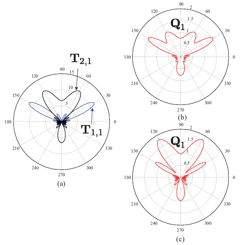
Refer to caption
Figure 4: Antenna radiation patterns.

Finally, we discuss the fact mentioned in Section 3.2 that the optimal transmit directions can be changed by the correlation pattern at the receiver side through βl,1​el,1\beta_{l,1}e_{l,1}. To understand this better, we consider two scenarios with K=1K=1, L=2L=2 and 𝐇¯=𝟎{\bar{{\bf H}}}={\bf 0}. The two scenarios use the same parameters except that the radiation patterns at the receiver of the second antenna set have different beam-widthes. Specifically, the radiation patterns at the receiver of the second antenna set have δ2,1𝖱=0.01\delta_{2,1}^{\sf R}=0.01 for scenario 1 and δ2,1𝖱=0.1\delta_{2,1}^{\sf R}=0.1 for scenario 2. We find it useful to observe the array patterns by plotting its array factor1010 10 Consider a uniform linear array with half wavelength spacing. Given a vector 𝐚∈ℂn×1{\bf a}\in{\mathbb{C}}^{n\times 1}, we can get its array factor in direction ϕ\phi by f⁡(ϕ)=∑l=1nai​e−𝗃​π​l​sin⁡(π​ϕ180).f(\phi)=\sum_{l=1}^{n}a_{i}e^{-{\sf j}\pi l\sin\left(\frac{\pi\phi}{180}\right)}. in all directions. The array patterns of 𝐓1,1{\bf T}_{1,1} and 𝐓2,1{\bf T}_{2,1} are depicted in Figure 4(a), where θ1,1𝖳=30∘\theta_{1,1}^{\sf T}=30^{\circ}, θ2,1𝖳=60∘\theta_{2,1}^{\sf T}=60^{\circ}, δ1,1𝖳=0.04\delta_{1,1}^{\sf T}=0.04, and δ2,1𝖳=0.03\delta_{2,1}^{\sf T}=0.03. The array patterns of the optimal input covariance 𝐐1{\bf Q}_{1} for the two scenarios are given in Figure 4(b) and (c), respectively. Figure 4(c) corresponds to the setting with the broader beamwidth of 𝐑2,1{\bf R}_{2,1}. In this case, the optimal covariance is shown to feed the signal largely according to 𝐓2,1{\bf T}_{2,1}, showing that the optimal transmit directions can be changed by the correlation pattern at the receiver side.

5 Conclusion

By using the large dimensional RMT, this paper investigated the deterministic equivalents for the large-scale MIMO MAC. The considered model includes the large-scale MIMO channel such as the general spatial correlation, the LOS components, and the channel entries being non-Gaussian. In particular, we derived the deterministic equivalent of the ergodic sum rate of the large-scale MIMO MAC. In addition, through the deterministic equivalent of the ergodic sum rate, we investigated the capacity-achieving input covariance matrices for the the large-scale MIMO MAC and proposed the iterative waterfilling algorithm for finding them. Finally, computer simulations were conducted to conclude the following three facts: First, the deterministic equivalent of the ergodic sum rate provides a very good approximation even when the numbers of antennas are of practical size. Second, calculating the ergodic sum rate by using the deterministic equivalent result is much more efficient than that by using the Monte-Carlo method when the system sizes are large. Hence, the deterministic equivalent result is of interest to addressing complex system optimization problems. Third, the optimal input covariance matrices predicted by the deterministic equivalent result are indeed remarkably close to those obtained by the corresponding finite-dimensional optimization approach, but in a much more efficient manner.

Investigation of the central limit theorem of the sum rate for the large-scale MIMO MAC by using the mathematical framework in [13], as well as application of the deterministic equivalent results to system-level designs [9, 23, 24, 25], are promising topics for future research.

Appendix

Appendix A Proof of 𝖤⁡{mℬN}−1N​𝗍𝗋​(𝚿)=O⁡(1N2){\sf E}\{m_{\boldsymbol{\cal B}_{N}}\}-\frac{1}{N}{\sf tr}\left({\boldsymbol{\Psi}}\right)=O\left(\frac{1}{N^{2}}\right) in Theorem 1

We start the proof by reformulating the channel model so that the derivation can be performed systematically. To this end, we denote

𝐑¯l,k\displaystyle{\underline{{\bf R}}}_{l,k} ≜𝖽𝗂𝖺𝗀⁡(𝟎N1,…,𝟎Nl−1,𝐑l,k,𝟎Nl+1,…,𝟎NL),\displaystyle\triangleq{\sf diag}\left({\bf 0}_{N_{1}},\dots,{\bf 0}_{N_{l-1}},{\bf R}_{l,k},{\bf 0}_{N_{l+1}},\dots,{\bf 0}_{N_{L}}\right), (39)
𝐓¯l,k\displaystyle{\underline{{\bf T}}}_{l,k} ≜𝖽𝗂𝖺𝗀⁡(𝟎n1,…,𝟎nk−1,𝐓l,k,𝟎nk+1,…,𝟎nK).\displaystyle\triangleq{\sf diag}\left({\bf 0}_{n_{1}},\dots,{\bf 0}_{n_{k-1}},{\bf T}_{l,k},{\bf 0}_{n_{k+1}},\dots,{\bf 0}_{n_{K}}\right). (40)

Also, let 𝐇¯¯l,k{\underline{{\bar{{\bf H}}}}}_{l,k} be the all-zero N×nN\times n matrix except that 𝐇l,k{\bf H}_{l,k} is used for its (∑i=1l−1Ni+1)(\sum_{i=1}^{l-1}N_{i}+1) to (∑i=1lNi)(\sum_{i=1}^{l}N_{i})-th row and (∑j=1k−1nj+1)(\sum_{j=1}^{k-1}n_{j}+1) to (∑j=1knj)(\sum_{j=1}^{k}n_{j})-th column. As a result, 𝐇{\bf H} is statistically equivalent to

𝐇=∑l,k𝐇¯l,k=∑l,k(𝐇¯~l,k+𝐇¯¯l,k),{\bf H}=\sum_{l,k}{\underline{{\bf H}}}_{l,k}=\sum_{l,k}\left({\underline{{\tilde{{\bf H}}}}}_{l,k}+{\underline{{\bar{{\bf H}}}}}_{l,k}\right), (41)

where 𝐇¯~l,k=𝐑¯l,k12​𝐗¯l,k​𝐓¯l,k12∈ℂN×n{\underline{{\tilde{{\bf H}}}}}_{l,k}={\underline{{\bf R}}}_{l,k}^{\frac{1}{2}}{\underline{{\bf X}}}_{l,k}{\underline{{\bf T}}}_{l,k}^{\frac{1}{2}}\in{\mathbb{C}}^{N\times n}, and 𝐗¯l,k≡[1nk​Xi​j(l,k)]∈ℂN×n{\underline{{\bf X}}}_{l,k}\equiv\left[\frac{1}{\sqrt{n_{k}}}X_{ij}^{(l,k)}\right]\in{\mathbb{C}}^{N\times n} consists of the random components of the channel. Here, 𝐗¯l,k{\underline{{\bf X}}}_{l,k}’s are assumed to be mutually independent. From (6), we have

𝐁N=(∑l,k(𝐑¯l,k12​𝐗¯l,k​𝐓¯l,k12+𝐇¯¯l,k))​(∑l,k(𝐑¯l,k12​𝐗¯l,k​𝐓¯l,k12+𝐇¯¯l,k))H{\bf B}_{N}=\left(\sum_{l,k}\left({\underline{{\bf R}}}_{l,k}^{\frac{1}{2}}{\underline{{\bf X}}}_{l,k}{\underline{{\bf T}}}_{l,k}^{\frac{1}{2}}+{\underline{{\bar{{\bf H}}}}}_{l,k}\right)\right)\left(\sum_{l,k}\left({\underline{{\bf R}}}_{l,k}^{\frac{1}{2}}{\underline{{\bf X}}}_{l,k}{\underline{{\bf T}}}_{l,k}^{\frac{1}{2}}+{\underline{{\bar{{\bf H}}}}}_{l,k}\right)\right)^{H} (42)

and

ℬN=(∑l,k(𝐑¯l,k12​𝒳¯l,k​𝐓¯l,k12+𝐇¯¯l,k))​(∑l,k(𝐑¯l,k12​𝒳¯l,k​𝐓¯l,k12+𝐇¯¯l,k))H,\boldsymbol{\cal B}_{N}=\left(\sum_{l,k}\left({\underline{{\bf R}}}_{l,k}^{\frac{1}{2}}{\underline{\boldsymbol{\cal X}}}_{l,k}{\underline{{\bf T}}}_{l,k}^{\frac{1}{2}}+{\underline{{\bar{{\bf H}}}}}_{l,k}\right)\right)\left(\sum_{l,k}\left({\underline{{\bf R}}}_{l,k}^{\frac{1}{2}}{\underline{\boldsymbol{\cal X}}}_{l,k}{\underline{{\bf T}}}_{l,k}^{\frac{1}{2}}+{\underline{{\bar{{\bf H}}}}}_{l,k}\right)\right)^{H}, (43)

where 𝐗¯l,k{\underline{{\bf X}}}_{l,k}’s and 𝒳¯l,k{\underline{\boldsymbol{\cal X}}}_{l,k}’s are matrices with entries satisfying Assumption 1 but 𝒳¯l,k{\underline{\boldsymbol{\cal X}}}_{l,k}’s are Gaussian.

Let 𝒮\boldsymbol{\cal S} and 𝒮~{\tilde{\boldsymbol{\cal S}}} be the resolvents of matrices 𝐇𝐇H{\bf H}{\bf H}^{H} and 𝐇H​𝐇{\bf H}^{H}{\bf H}, respectively, given by

𝒮\displaystyle\boldsymbol{\cal S} ≜(𝐇𝐇H+ω​𝐈N)−1,\displaystyle\triangleq\left({\bf H}{\bf H}^{H}+\omega{\bf I}_{N}\right)^{-1}, (44)
𝒮~\displaystyle{\tilde{\boldsymbol{\cal S}}} ≜(𝐇H​𝐇+ω​𝐈n)−1.\displaystyle\triangleq\left({\bf H}^{H}{\bf H}+\omega{\bf I}_{n}\right)^{-1}. (45)

These resolvents clearly satisfy the following useful properties:

𝒮⪯1ω​𝐈N,and​𝒮~⪯1ω​𝐈n.\boldsymbol{\cal S}\preceq\frac{1}{\omega}{\bf I}_{N},~~\mbox{and}~~{\tilde{\boldsymbol{\cal S}}}\preceq\frac{1}{\omega}{\bf I}_{n}. (46)

To facilitate our notations, we use 𝑎∘\mathrel{\mathop{\kern 0.0pta}\limits^{\circ}} to denote the zero-mean random variable a−𝖤​{a}a-{\sf E}\{a\}, where aa is a random variable. To accomplish the proof, the following two lemmas are useful.

Lemma 1

(Integration by Parts Formula for Gaussian Functionals) (see, e.g., [27, Proposition 2.4]) Let 𝛏=[ξ1,…,ξM]T{\boldsymbol{\xi}}=[\xi_{1},\ldots,\xi_{M}]^{T} be a complex Gaussian random vector such that 𝖤​{𝛏}=𝟎{\sf E}\{{\boldsymbol{\xi}}\}={\bf 0} and 𝖤​{𝛏​𝛏H}=𝛀{\sf E}\{{\boldsymbol{\xi}}{\boldsymbol{\xi}}^{H}\}={\boldsymbol{\Omega}}. Denoting by Γ⁡(𝛏)\Gamma({\boldsymbol{\xi}}) a complex function polynomially bounded with its derivatives, we have

𝖤⁡{ξp​Γ​(𝝃)}=∑m=1MΩp​m​𝖤​{Γ⁡(𝝃)∂ξm∗}.{\sf E}\left\{\xi_{p}\Gamma({\boldsymbol{\xi}})\right\}=\sum_{m=1}^{M}\Omega_{pm}{\sf E}\left\{\frac{\Gamma({\boldsymbol{\xi}})}{\partial\xi_{m}^{*}}\right\}. (47)
Lemma 2

(The Poincaré-Nash Inequality) (see, e.g., [27, Proposition 2.5]) Let 𝛏=[ξ1,…,ξM]T{\boldsymbol{\xi}}=[\xi_{1},\ldots,\xi_{M}]^{T} be a complex Gaussian random vector such that 𝖤​{𝛏}=𝟎{\sf E}\{{\boldsymbol{\xi}}\}={\bf 0} and 𝖤​{𝛏​𝛏H}=𝛀{\sf E}\{{\boldsymbol{\xi}}{\boldsymbol{\xi}}^{H}\}={\boldsymbol{\Omega}}. Denoting by Γ⁡(𝛏)\Gamma({\boldsymbol{\xi}}) a complex function polynomially bounded with its derivatives, the following inequality holds true:

𝖵𝖺𝗋(Γ(𝝃))≤𝖤{(▽ξΓ(𝝃))T𝛀(▽ξΓ(𝝃))∗}+𝖤{(▽ξ∗Γ(𝝃))H𝛀(▽ξ∗Γ(𝝃))},{\sf Var}\left(\Gamma({\boldsymbol{\xi}})\right)\leq{\sf E}\left\{\left(\bigtriangledown_{\xi}\Gamma({\boldsymbol{\xi}})\right)^{T}{\boldsymbol{\Omega}}\left(\bigtriangledown_{\xi}\Gamma({\boldsymbol{\xi}})\right)^{*}\right\}+{\sf E}\left\{\left(\bigtriangledown_{\xi^{*}}\Gamma({\boldsymbol{\xi}})\right)^{H}{\boldsymbol{\Omega}}\left(\bigtriangledown_{\xi^{*}}\Gamma({\boldsymbol{\xi}})\right)\right\}, (48)

where ▽ξΓ(𝛏)=[∂Γ∂ξ1,…,∂Γ∂ξM]T\bigtriangledown_{\xi}\Gamma({\boldsymbol{\xi}})=\left[\frac{\partial\Gamma}{\partial\xi_{1}},\dots,\frac{\partial\Gamma}{\partial\xi_{M}}\right]^{T} and ▽ξ∗Γ(𝛏)=[∂Γ∂ξ1∗,…,∂Γ∂ξM∗]T\bigtriangledown_{\xi^{*}}\Gamma({\boldsymbol{\xi}})=\left[\frac{\partial\Gamma}{\partial\xi_{1}^{*}},\dots,\frac{\partial\Gamma}{\partial\xi_{M}^{*}}\right]^{T}.

The rigorous proof of Theorem 1 is rather complex. Although a standard procedure for the MIMO channel without the LOS components [18] is used, several additional manipulations for the LOS components to our present argument are required. To show this, we split the proof into two steps: First, we prove that 𝗍𝗋⁡(𝖤​{𝒮}−𝚿)→0{\sf tr}\left({\sf E}\{\boldsymbol{\cal S}\}-{\boldsymbol{\Psi}}\right)\rightarrow 0; secondly, we refine the convergence rate that 1N​(𝗍𝗋⁡(𝖤⁡{𝒮}−𝚿))=O⁡(1N2)\frac{1}{N}\left({\sf tr}\left({\sf E}\{\boldsymbol{\cal S}\}-{\boldsymbol{\Psi}}\right)\right)=O\left(\frac{1}{N^{2}}\right). However, it is difficult to prove directly that 𝗍𝗋⁡(𝖤​{𝒮}−𝚿)→0{\sf tr}\left({\sf E}\{\boldsymbol{\cal S}\}-{\boldsymbol{\Psi}}\right)\rightarrow 0. To that end, we employ an intermediate quantity between 𝖤​{𝒮}{\sf E}\{\boldsymbol{\cal S}\} and 𝚿{\boldsymbol{\Psi}} and establish the following two propositions.

Proposition 3

As 𝒩→∞\mbox{${\cal N}$}\rightarrow\infty, we have

𝗍𝗋⁡(𝖤​{𝒮}−𝚵)\displaystyle{\sf tr}{({\sf E}{\{\boldsymbol{\cal S}\}}-{\boldsymbol{\Xi}})} ⟶0,\displaystyle\longrightarrow 0, (49a)
𝗍𝗋⁡(𝖤​{𝒮~}−𝚵~)\displaystyle{\sf tr}{({\sf E}{\{{\tilde{\boldsymbol{\cal S}}}\}}-{\tilde{{\boldsymbol{\Xi}}}})} ⟶0,\displaystyle\longrightarrow 0, (49b)

where

𝚵\displaystyle{\boldsymbol{\Xi}} ≜[ω⁡(𝐈N+𝖽𝗂𝖺𝗀⁡({∑k=1Kα~l,k​𝐑l,k}∀l)+𝐇¯​𝚯~​𝐇¯H)]−1,\displaystyle\triangleq\left[\omega\left({\bf I}_{N}+{\sf diag}\left(\left\{\sum_{k=1}^{K}{\tilde{\alpha}}_{l,k}{\bf R}_{l,k}\right\}_{\forall l}\right)+{\bar{{\bf H}}}{\tilde{{\boldsymbol{\Theta}}}}{\bar{{\bf H}}}^{H}\right)\right]^{-1}, (50a)
𝚵~\displaystyle{\tilde{{\boldsymbol{\Xi}}}} ≜[ω⁡(𝐈n+𝖽𝗂𝖺𝗀⁡({∑l=1Lαl,k​𝐓l,k}∀k)+𝐇¯H​𝚯​𝐇¯)]−1,\displaystyle\triangleq\left[\omega\left({\bf I}_{n}+{\sf diag}\left(\left\{\sum_{l=1}^{L}\alpha_{l,k}{\bf T}_{l,k}\right\}_{\forall k}\right)+{\bar{{\bf H}}}^{H}{\boldsymbol{\Theta}}{\bar{{\bf H}}}\right)\right]^{-1}, (50b)
𝚯\displaystyle{\boldsymbol{\Theta}} ≜𝖽𝗂𝖺𝗀⁡(𝚯1,…,𝚯L),\displaystyle\triangleq{\sf diag}\left({\boldsymbol{\Theta}}_{1},\dots,{\boldsymbol{\Theta}}_{L}\right), (50c)
𝚯~\displaystyle{\tilde{{\boldsymbol{\Theta}}}} ≜𝖽𝗂𝖺𝗀⁡(𝚯~1,…,𝚯~K),\displaystyle\triangleq{\sf diag}({\tilde{{\boldsymbol{\Theta}}}}_{1},\dots,{\tilde{{\boldsymbol{\Theta}}}}_{K}), (50d)
𝚯l\displaystyle{\boldsymbol{\Theta}}_{l} ≜[ω(𝐈+∑k=1Kα~l,k𝐑l,k)]−1,for l=1,…,L,\displaystyle\triangleq\left[\omega\left({\bf I}+\sum_{k=1}^{K}{\tilde{\alpha}}_{l,k}{\bf R}_{l,k}\right)\right]^{-1},~\mbox{for }l=1,\dots,L, (50e)
𝚯~k\displaystyle{\tilde{{\boldsymbol{\Theta}}}}_{k} ≜[ω(𝐈+∑l=1Lαl,k𝐓l,k)]−1,for k=1,…,K,\displaystyle\triangleq\left[\omega\left({\bf I}+\sum_{l=1}^{L}\alpha_{l,k}{\bf T}_{l,k}\right)\right]^{-1},~\mbox{for }k=1,\dots,K, (50f)
αl,k\displaystyle\alpha_{l,k} ≜1nk​𝗍𝗋​(𝐑l,k​𝖤​{⟨⟨𝒮⟩⟩l}),\displaystyle\triangleq\frac{1}{n_{k}}{\sf tr}{({\bf R}_{l,k}{\sf E}{\{\mbox{$\langle\!\langle\boldsymbol{\cal S}\rangle\!\rangle$}_{l}\}})}, (50g)
α~l,k\displaystyle{\tilde{\alpha}}_{l,k} ≜1nk​𝗍𝗋​(𝐓l,k​𝖤​{⟨𝒮~⟩k}).\displaystyle\triangleq\frac{1}{n_{k}}{\sf tr}{({\bf T}_{l,k}{\sf E}{\{\mbox{$\langle{\tilde{\boldsymbol{\cal S}}}\rangle$}_{k}\}})}. (50h)

Proof: See Appendix A.1.  □\square

Proposition 4

As 𝒩→∞\mbox{${\cal N}$}\rightarrow\infty, we have

𝗍𝗋⁡(𝚵−𝚿)\displaystyle{\sf tr}{({\boldsymbol{\Xi}}-{\boldsymbol{\Psi}})} ⟶0,\displaystyle\longrightarrow 0, (51a)
𝗍𝗋⁡(𝚵~−𝚿~)\displaystyle{\sf tr}{({\tilde{{\boldsymbol{\Xi}}}}-{\tilde{{\boldsymbol{\Psi}}}})} ⟶0.\displaystyle\longrightarrow 0. (51b)

Proof: See Appendix A.2.  □\square

From (49a) to (51a), the proof of 𝖤⁡{mℬN}−1N​𝗍𝗋​(𝚿)→0{\sf E}\{m_{\boldsymbol{\cal B}_{N}}\}-\frac{1}{N}{\sf tr}\left({\boldsymbol{\Psi}}\right)\rightarrow 0 can be accomplished.

Proposition 5

As 𝒩→∞\mbox{${\cal N}$}\rightarrow\infty, we have

1N​𝗍𝗋​(𝖤​{𝒮}−𝚵)\displaystyle\frac{1}{N}{\sf tr}{\left({\sf E}{\left\{\boldsymbol{\cal S}\right\}}-{\boldsymbol{\Xi}}\right)} =O⁡(1N2),\displaystyle=O\left(\frac{1}{N^{2}}\right), (52a)
1N​𝗍𝗋​(𝖤​{𝒮~}−𝚵~)\displaystyle\frac{1}{N}{\sf tr}{({\sf E}{\{{\tilde{\boldsymbol{\cal S}}}\}}-{\tilde{{\boldsymbol{\Xi}}}})} =O⁡(1N2),\displaystyle=O\left(\frac{1}{N^{2}}\right), (52b)
1N​𝗍𝗋​(𝚵−𝚿)\displaystyle\frac{1}{N}{\sf tr}{\left({\boldsymbol{\Xi}}-{\boldsymbol{\Psi}}\right)} =O⁡(1N2),\displaystyle=O\left(\frac{1}{N^{2}}\right), (52c)
1N​𝗍𝗋​(𝚵~−𝚿~)\displaystyle\frac{1}{N}{\sf tr}{({\tilde{{\boldsymbol{\Xi}}}}-{\tilde{{\boldsymbol{\Psi}}}})} =O⁡(1N2).\displaystyle=O\left(\frac{1}{N^{2}}\right). (52d)

Proof: See Appendix A.3.  □\square

Consequently, (17) then follows from (52a) and (52c). The proof is complete.

A.1 Proof of Proposition 3

From (41) and (44), we have

𝒮=1ω​𝐈N−1ω​𝒮​𝐇𝐇H=1ω​𝐈N−1ω​∑l1,k1∑l,k𝒮​𝐇¯l1,k1​𝐇¯l,kH,\boldsymbol{\cal S}=\frac{1}{\omega}{\bf I}_{N}-\frac{1}{\omega}{\boldsymbol{\cal S}{\bf H}{\bf H}^{H}}=\frac{1}{\omega}{\bf I}_{N}-\frac{1}{\omega}\sum_{l_{1},k_{1}}\sum_{l,k}\boldsymbol{\cal S}{\underline{{\bf H}}}_{l_{1},k_{1}}{\underline{{\bf H}}}_{l,k}^{H}, (53)

and

𝖤​{𝒮p​q}=\displaystyle{\sf E}\{{\mathcal{S}}_{pq}\}= 1ω​δp​q−1ω​𝖤​{[𝒮​𝐇𝐇H]p​q}\displaystyle\frac{1}{\omega}\delta_{pq}-\frac{1}{\omega}{\sf E}{\left\{[\boldsymbol{\cal S}{\bf H}{\bf H}^{H}]_{pq}\right\}} (54)
=\displaystyle= 1ω​δp​q−1ω​∑l,k𝖤⁡{[𝒮​𝐇¯l,k​𝐇¯l,kH]p​q}−1ω​∑l≠l1L∑k≠k1K𝖤⁡{[𝒮​𝐇¯l,k​𝐇¯l1,k1H]p​q}.\displaystyle\frac{1}{\omega}\delta_{pq}-\frac{1}{\omega}\sum_{l,k}{\sf E}{\left\{[\boldsymbol{\cal S}{\underline{{\bf H}}}_{l,k}{\underline{{\bf H}}}_{l,k}^{H}]_{pq}\right\}}-\frac{1}{\omega}\sum_{l\neq l_{1}}^{L}\sum_{k\neq k_{1}}^{K}{\sf E}{\left\{[\boldsymbol{\cal S}{\underline{{\bf H}}}_{l,k}{\underline{{\bf H}}}_{l_{1},k_{1}}^{H}]_{pq}\right\}}. (55)

We first calculate 𝖤⁡{[𝒮​𝐇𝐇H]p​q}{\sf E}{\left\{[\boldsymbol{\cal S}{\bf H}{\bf H}^{H}]_{pq}\right\}}. Using the integration by parts formula (47), we write

𝖤{𝒮p​iH¯i​j(l,k)H¯q​r(l,k)∗}=\displaystyle{\sf E}{\left\{{\mathcal{S}}_{pi}{\underline{H}}_{ij}^{(l,k)}{\underline{H}}_{qr}^{(l,k)*}\right\}}= 𝖤{𝒮p​iH¯~i​j(l,k)H¯q​r(l,k)∗}+𝖤{𝒮p​iH¯~q​r(l,k)∗}H¯¯i​j(l,k)+𝖤{𝒮p​i}H¯¯i​j(l,k)H¯¯q​r(l,k)∗\displaystyle{\sf E}{\left\{{\mathcal{S}}_{pi}{\underline{{\tilde{H}}}}_{ij}^{(l,k)}{\underline{H}}_{qr}^{(l,k)*}\right\}}+{\sf E}{\left\{{\mathcal{S}}_{pi}{\underline{{\tilde{H}}}}_{qr}^{(l,k)*}\right\}}\underline{\bar{H}}_{ij}^{(l,k)}+{\sf E}{\left\{{\mathcal{S}}_{pi}\right\}}{\underline{{\bar{H}}}}_{ij}^{(l,k)}{\underline{{\bar{H}}}}_{qr}^{(l,k)*}
=\displaystyle= 1nk∑m,nR¯i​m(l,k)T¯j​n(l,k)∗𝖤{∂𝒮p​iH¯q​r(l,k)∗∂H¯~m​n(l,k)∗}+1nk∑m,nR¯q​m(l,k)∗T¯r​n(l,k)𝖤{∂𝒮p​i∂H¯~m​n(l,k)}H¯¯i​j(l,k)\displaystyle\frac{1}{n_{k}}\sum_{m,n}{\underline{R}}_{im}^{(l,k)}{\underline{T}}_{jn}^{(l,k)*}{\sf E}{\left\{\frac{\partial{\mathcal{S}}_{pi}{\underline{H}}_{qr}^{(l,k)*}}{\partial{\underline{{\tilde{H}}}}_{mn}^{(l,k)*}}\right\}}+\frac{1}{n_{k}}\sum_{m,n}{\underline{R}}_{qm}^{(l,k)*}{\underline{T}}_{rn}^{(l,k)}{\sf E}{\left\{\frac{\partial{\mathcal{S}}_{pi}}{\partial{\underline{{\tilde{H}}}}_{mn}^{(l,k)}}\right\}}{\underline{{\bar{H}}}}_{ij}^{(l,k)}
+𝖤{𝒮p​i}H¯¯i​j(l,k)H¯¯q​r(l,k)∗,\displaystyle+{\sf E}{\{{\mathcal{S}}_{pi}\}}{\underline{{\bar{H}}}}_{ij}^{(l,k)}{\underline{{\bar{H}}}}_{qr}^{(l,k)*}, (56)

and similarly,

𝖤{𝒮p​iH¯i​j(l,k)H¯q​r(l1,k1)∗}=1nk∑m,nR¯i​m(l,k)T¯j​n(l,k)∗𝖤{∂𝒮p​i∂H¯~m​n(l,k)∗}H¯q​r(l1,k1)∗+1nk1∑m,nR¯q​m(l1,k1)∗T¯r​n(l1,k1)𝖤{∂𝒮p​i∂H¯~m​n(l1,k1)}H¯¯i​j(l,k)+𝖤{𝒮p​i}H¯¯i​j(l,k)H¯¯q​r(l1,k1)∗.{\sf E}{\left\{{\mathcal{S}}_{pi}{\underline{H}}_{ij}^{(l,k)}{\underline{H}}_{qr}^{(l_{1},k_{1})*}\right\}}=\frac{1}{n_{k}}\sum_{m,n}{\underline{R}}_{im}^{(l,k)}{\underline{T}}_{jn}^{(l,k)*}{\sf E}{\left\{\frac{\partial{\mathcal{S}}_{pi}}{\partial{\underline{{\tilde{H}}}}_{mn}^{(l,k)*}}\right\}{\underline{H}}_{qr}^{(l_{1},k_{1})*}}\\ +\frac{1}{n_{k_{1}}}\sum_{m,n}{\underline{R}}_{qm}^{(l_{1},k_{1})*}{\underline{T}}_{rn}^{(l_{1},k_{1})}{\sf E}{\left\{\frac{\partial{\mathcal{S}}_{pi}}{\partial{\underline{{\tilde{H}}}}_{mn}^{(l_{1},k_{1})}}\right\}}{\underline{{\bar{H}}}}_{ij}^{(l,k)}+{\sf E}{\{{\mathcal{S}}_{pi}\}}{\underline{{\bar{H}}}}_{ij}^{(l,k)}{\underline{{\bar{H}}}}_{qr}^{(l_{1},k_{1})*}. (57)

Now, using the fact that

𝖤​{∂𝒮p​i∂H¯~m​n(l,k)}\displaystyle{\sf E}\left\{\frac{\partial{\mathcal{S}}_{pi}}{\partial{\underline{{\tilde{H}}}}_{mn}^{(l,k)}}\right\} =−𝖤⁡{𝒮p​m​[𝐇H​𝒮]n​i},\displaystyle=-{\sf E}\left\{{\mathcal{S}}_{pm}[{\bf H}^{H}\boldsymbol{\cal S}]_{ni}\right\}, (58a)
𝖤​{∂𝒮p​i∂H¯~m​n(l,k)∗}\displaystyle{\sf E}\left\{\frac{\partial{\mathcal{S}}_{pi}}{\partial{\underline{{\tilde{H}}}}_{mn}^{(l,k)*}}\right\} =−𝖤⁡{𝒮m​i​[𝒮​𝐇]p​n},\displaystyle=-{\sf E}\left\{{\mathcal{S}}_{mi}[\boldsymbol{\cal S}{\bf H}]_{pn}\right\}, (58b)
𝖤​{∂𝒮p​iH¯q​r(l,k)∗∂H¯~m​n(l,k)∗}\displaystyle{\sf E}\left\{\frac{\partial{\mathcal{S}}_{pi}{\underline{H}}_{qr}^{(l,k)*}}{\partial{\underline{{\tilde{H}}}}_{mn}^{(l,k)*}}\right\} =𝖤{𝒮p​iδq​mδr​n−𝒮m​i[𝒮𝐇]p​nH¯q​r(l,k)∗},\displaystyle={\sf E}\left\{{\mathcal{S}}_{pi}\delta_{qm}\delta_{rn}-{\mathcal{S}}_{mi}[\boldsymbol{\cal S}{\bf H}]_{pn}{\underline{H}}_{qr}^{(l,k)*}\right\}, (58c)

we have

𝖤{𝒮p​iH¯i​j(l,k)H¯q​r(l,k)∗}=1nkR¯i​q(l,k)T¯j​r(l,k)∗𝖤{𝒮p​i}−1nk𝖤{[𝐑¯l,k𝒮]i​i[𝒮𝐇𝐓¯l,k]p​jH¯q​r(l,k)∗}−1nk𝖤{[𝒮𝐑¯l,k]p​q[𝐓¯l,k𝐇H𝒮]r​i}H¯¯i​j(l,k)+𝖤{𝒮p​i}H¯¯i​j(l,k)H¯¯q​r(l,k)∗,{\sf E}{\left\{{\mathcal{S}}_{pi}{\underline{H}}_{ij}^{(l,k)}{\underline{H}}_{qr}^{(l,k)*}\right\}}=\frac{1}{n_{k}}{\underline{R}}_{iq}^{(l,k)}{\underline{T}}_{jr}^{(l,k)*}{\sf E}{\{{\mathcal{S}}_{pi}\}}-\frac{1}{n_{k}}{\sf E}{\left\{[{\underline{{\bf R}}}_{l,k}\boldsymbol{\cal S}]_{ii}[\boldsymbol{\cal S}{\bf H}{\underline{{\bf T}}}_{l,k}]_{pj}{\underline{H}}_{qr}^{(l,k)*}\right\}}\\ -\frac{1}{n_{k}}{\sf E}{\left\{[{\mathcal{S}}{\underline{{\bf R}}}_{l,k}]_{pq}[{\underline{{\bf T}}}_{l,k}{\bf H}^{H}\boldsymbol{\cal S}]_{ri}\right\}}{\underline{{\bar{H}}}}_{ij}^{(l,k)}+{\sf E}{\{{\mathcal{S}}_{pi}\}}{\underline{{\bar{H}}}}_{ij}^{(l,k)}{\underline{{\bar{H}}}}_{qr}^{(l,k)*}, (59)

and

𝖤{𝒮p​iH¯i​j(l,k)H¯q​r(l1,k1)∗}=−1nk𝖤{[𝐑¯l,k𝒮]i​i[𝒮𝐇𝐓¯l,k]p​jH¯q​r(l1,k1)∗}−1nk1𝖤{[𝒮𝐑¯l1,k1]p​q[𝐓¯l1,k1𝐇H𝒮]r​i}H¯¯i​j(l,k)+𝖤{𝒮p​i}H¯¯i​j(l,k)H¯¯q​r(l1,k1)∗.{\sf E}{\left\{{\mathcal{S}}_{pi}{\underline{H}}_{ij}^{(l,k)}{\underline{H}}_{qr}^{(l_{1},k_{1})*}\right\}}=-\frac{1}{n_{k}}{\sf E}{\left\{[{\underline{{\bf R}}}_{l,k}\boldsymbol{\cal S}]_{ii}[\boldsymbol{\cal S}{\bf H}{\underline{{\bf T}}}_{l,k}]_{pj}{\underline{H}}_{qr}^{(l_{1},k_{1})*}\right\}}\\ -\frac{1}{n_{k_{1}}}{\sf E}{\left\{[{\mathcal{S}}{\underline{{\bf R}}}_{l_{1},k_{1}}]_{pq}[{\underline{{\bf T}}}_{l_{1},k_{1}}{\bf H}^{H}\boldsymbol{\cal S}]_{ri}\right\}}{\underline{{\bar{H}}}}_{ij}^{(l,k)}+{\sf E}{\{{\mathcal{S}}_{pi}\}}{\underline{{\bar{H}}}}_{ij}^{(l,k)}{\underline{{\bar{H}}}}_{qr}^{(l_{1},k_{1})*}. (60)

Then, summing over ii, we have

𝖤{[𝒮𝐇¯l,k]p​jH¯q​r(l,k)∗}=1nkT¯j​r(l,k)∗𝖤{[𝒮𝐑¯l,k]p​q}−1nk𝖤{𝗍𝗋(𝐑¯l,k𝒮)[𝒮𝐇𝐓¯l,k]p​jH¯q​r(l,k)∗}−1nk𝖤{[𝒮𝐑¯l,k]p​q[𝐓¯l,k𝐇H𝒮𝐇¯¯l,k]r​j}+𝖤{[𝒮𝐇¯¯l,k]p​j}H¯¯q​r(l,k)∗,{\sf E}{\left\{[\boldsymbol{\cal S}{\underline{{\bf H}}}_{l,k}]_{pj}{\underline{H}}_{qr}^{(l,k)*}\right\}}=\frac{1}{n_{k}}{\underline{T}}_{jr}^{(l,k)*}{\sf E}{\{[\boldsymbol{\cal S}{\underline{{\bf R}}}_{l,k}]_{pq}\}}-\frac{1}{n_{k}}{\sf E}{\left\{{\sf tr}({\underline{{\bf R}}}_{l,k}\boldsymbol{\cal S})[\boldsymbol{\cal S}{\bf H}{\underline{{\bf T}}}_{l,k}]_{pj}{\underline{H}}_{qr}^{(l,k)*}\right\}}\\ -\frac{1}{n_{k}}{\sf E}{\left\{[\boldsymbol{\cal S}{\underline{{\bf R}}}_{l,k}]_{pq}[{\underline{{\bf T}}}_{l,k}{\bf H}^{H}\boldsymbol{\cal S}{\underline{{\bar{{\bf H}}}}}_{l,k}]_{rj}\right\}}+{\sf E}\{[\boldsymbol{\cal S}{\underline{{\bar{{\bf H}}}}}_{l,k}]_{pj}\}{\underline{{\bar{H}}}}_{qr}^{(l,k)*}, (61)

and

𝖤{[𝒮𝐇¯l,k]p​jH¯q​r(l1,k1)∗}=−1nk𝖤{𝗍𝗋(𝐑¯l,k𝒮)[𝒮𝐇𝐓¯l,k]p​jH¯q​r(l1,k1)∗}−1nk1𝖤{[𝒮𝐑¯l1,k1]p​q[𝐓¯l1,k1𝐇H𝒮𝐇¯¯l,k]r​j𝒮p​m}+𝖤{[𝒮𝐇¯¯l,k]p​j}H¯¯q​r(l1,k1)∗.{\sf E}{\left\{[\boldsymbol{\cal S}{\underline{{\bf H}}}_{l,k}]_{pj}{\underline{H}}_{qr}^{(l_{1},k_{1})*}\right\}}=-\frac{1}{n_{k}}{\sf E}{\left\{{\sf tr}({\underline{{\bf R}}}_{l,k}\boldsymbol{\cal S})[\boldsymbol{\cal S}{\bf H}{\underline{{\bf T}}}_{l,k}]_{pj}{\underline{H}}_{qr}^{(l_{1},k_{1})*}\right\}}\\ -\frac{1}{n_{k_{1}}}{\sf E}{\left\{[\boldsymbol{\cal S}{\underline{{\bf R}}}_{l_{1},k_{1}}]_{pq}[{\underline{{\bf T}}}_{l_{1},k_{1}}{\bf H}^{H}\boldsymbol{\cal S}{\underline{{\bar{{\bf H}}}}}_{l,k}]_{rj}{\mathcal{S}}_{pm}\right\}}+{\sf E}\left\{[\boldsymbol{\cal S}{\underline{{\bar{{\bf H}}}}}_{l,k}]_{pj}\right\}{\underline{{\bar{H}}}}_{qr}^{(l_{1},k_{1})*}. (62)

Let αl,k≜1nk​𝗍𝗋​(𝐑¯l,k​𝖤​{𝒮})=1nk​𝗍𝗋​(𝐑l,k​𝖤​{⟨⟨𝒮⟩⟩l})\alpha_{l,k}\triangleq\frac{1}{n_{k}}{\sf tr}{\left({\underline{{\bf R}}}_{l,k}{\sf E}{\{\boldsymbol{\cal S}\}}\right)}=\frac{1}{n_{k}}{\sf tr}{\left({\bf R}_{l,k}{\sf E}{\{\mbox{$\langle\!\langle\boldsymbol{\cal S}\rangle\!\rangle$}_{l}\}}\right)} and 𝜂∘l,k≜1nk𝗍𝗋(𝐑¯l,k𝒮)−αl,k\mathrel{\mathop{\kern 0.0pt\eta}\limits^{\circ}}_{l,k}\triangleq\frac{1}{n_{k}}{\sf tr}{\left({\underline{{\bf R}}}_{l,k}\boldsymbol{\cal S}\right)}-\alpha_{l,k}. Then, we get

𝖤{[𝒮𝐇¯l,k]p​jH¯q​r(l,k)∗}=1nkT¯j​r(l,k)∗𝖤{[𝒮𝐑¯l,k]p​q}−αl,k𝖤{[𝒮𝐇𝐓¯l,k]p​jH¯q​r(l,k)∗}−𝖤{𝜂∘l,k[𝒮𝐇𝐓¯l,k]p​jH¯q​r(l,k)∗}−1nk𝖤{[𝒮𝐑¯l,k]p​q[𝐓¯l,k𝐇H𝒮𝐇¯¯l,k]r​j}+𝖤{[𝒮𝐇¯¯l,k]p​j}H¯¯q​r(l,k)∗,{\sf E}{\left\{[\boldsymbol{\cal S}{\underline{{\bf H}}}_{l,k}]_{pj}{\underline{H}}_{qr}^{(l,k)*}\right\}}=\frac{1}{n_{k}}{\underline{T}}_{jr}^{(l,k)*}{\sf E}{\{[\boldsymbol{\cal S}{\underline{{\bf R}}}_{l,k}]_{pq}\}}-\alpha_{l,k}{\sf E}{\left\{[\boldsymbol{\cal S}{\bf H}{\underline{{\bf T}}}_{l,k}]_{pj}{\underline{H}}_{qr}^{(l,k)*}\right\}}-{\sf E}{\left\{\mathrel{\mathop{\kern 0.0pt\eta}\limits^{\circ}}_{l,k}[\boldsymbol{\cal S}{\bf H}{\underline{{\bf T}}}_{l,k}]_{pj}{\underline{H}}_{qr}^{(l,k)*}\right\}}\\ -\frac{1}{n_{k}}{\sf E}{\left\{[\boldsymbol{\cal S}{\underline{{\bf R}}}_{l,k}]_{pq}[{\underline{{\bf T}}}_{l,k}{\bf H}^{H}\boldsymbol{\cal S}{\underline{{\bar{{\bf H}}}}}_{l,k}]_{rj}\right\}}+{\sf E}\{[\boldsymbol{\cal S}{\underline{{\bar{{\bf H}}}}}_{l,k}]_{pj}\}{\underline{{\bar{H}}}}_{qr}^{(l,k)*}, (63)

and

𝖤{[𝒮𝐇¯l,k]p​jH¯q​r(l1,k1)∗}=−αl,k𝖤{[𝒮𝐇𝐓¯l,k]p​jH¯q​r(l1,k1)∗}−𝖤{𝜂∘l,k[𝒮𝐇𝐓¯l,k]p​jH¯q​r(l1,k1)∗}−1nk1𝖤{[𝒮𝐑¯l1,k1]p​q[𝐓¯l1,k1𝐇H𝒮𝐇¯¯l,k]r​j}+𝖤{[𝒮𝐇¯¯l,k]p​j}H¯¯q​r(l1,k1)∗.{\sf E}{\left\{[\boldsymbol{\cal S}{\underline{{\bf H}}}_{l,k}]_{pj}{\underline{H}}_{qr}^{(l_{1},k_{1})*}\right\}}=-\alpha_{l,k}{\sf E}{\left\{[\boldsymbol{\cal S}{\bf H}{\underline{{\bf T}}}_{l,k}]_{pj}{\underline{H}}_{qr}^{(l_{1},k_{1})*}\right\}}-{\sf E}{\left\{\mathrel{\mathop{\kern 0.0pt\eta}\limits^{\circ}}_{l,k}[\boldsymbol{\cal S}{\bf H}{\underline{{\bf T}}}_{l,k}]_{pj}{\underline{H}}_{qr}^{(l_{1},k_{1})*}\right\}}\\ -\frac{1}{n_{k_{1}}}{\sf E}{\left\{[\boldsymbol{\cal S}{\underline{{\bf R}}}_{l_{1},k_{1}}]_{pq}[{\underline{{\bf T}}}_{l_{1},k_{1}}{\bf H}^{H}\boldsymbol{\cal S}{\underline{{\bar{{\bf H}}}}}_{l,k}]_{rj}\right\}}+{\sf E}\{[\boldsymbol{\cal S}{\underline{{\bar{{\bf H}}}}}_{l,k}]_{pj}\}{\underline{{\bar{H}}}}_{qr}^{(l_{1},k_{1})*}. (64)

From (63) and (64), we obtain

𝖤{[𝒮𝐇]p​jHq​r∗}=∑l,k1nkT¯j​r(l,k)∗𝖤{[𝒮𝐑¯l,k]p​q}−∑l,kαl,k𝖤{[𝒮𝐇𝐓¯l,k]p​jHq​r∗}−∑l,k𝖤{𝜂∘l,k[𝒮𝐇𝐓¯l,k]p​jHq​r∗}−∑l1,k11nk1𝖤{[𝒮𝐑¯l1,k1]p​q[𝐓¯l1,k1𝐇H𝒮𝐇¯]r​j}+𝖤{[𝒮𝐇¯]p​j}H¯q​r∗.{\sf E}{\left\{[\boldsymbol{\cal S}{\bf H}]_{pj}H_{qr}^{*}\right\}}=\sum_{l,k}\frac{1}{n_{k}}{\underline{T}}_{jr}^{(l,k)*}{\sf E}{\{[\boldsymbol{\cal S}{\underline{{\bf R}}}_{l,k}]_{pq}\}}-\sum_{l,k}\alpha_{l,k}{\sf E}{\left\{[\boldsymbol{\cal S}{\bf H}{\underline{{\bf T}}}_{l,k}]_{pj}H_{qr}^{*}\right\}}\\ -\sum_{l,k}{\sf E}{\left\{\mathrel{\mathop{\kern 0.0pt\eta}\limits^{\circ}}_{l,k}[\boldsymbol{\cal S}{\bf H}{\underline{{\bf T}}}_{l,k}]_{pj}H_{qr}^{*}\right\}}-\sum_{l_{1},k_{1}}\frac{1}{n_{k_{1}}}{\sf E}{\left\{[\boldsymbol{\cal S}{\underline{{\bf R}}}_{l_{1},k_{1}}]_{pq}[{\underline{{\bf T}}}_{l_{1},k_{1}}{\bf H}^{H}\boldsymbol{\cal S}{\bar{{\bf H}}}]_{rj}\right\}}+{\sf E}\{[\boldsymbol{\cal S}{\bar{{\bf H}}}]_{pj}\}{\bar{H}}_{qr}^{*}. (65)

Defining

𝚯~≜[ω⁡(𝐈n+∑l,kαl,k​𝐓¯l,k)]−1=𝖽𝗂𝖺𝗀⁡(𝚯~1,…,𝚯~K),{\tilde{{\boldsymbol{\Theta}}}}\triangleq\left[\omega\left({\bf I}_{n}+\sum_{l,k}\alpha_{l,k}{\underline{{\bf T}}}_{l,k}\right)\right]^{-1}={\sf diag}\left({\tilde{{\boldsymbol{\Theta}}}}_{1},\ldots,{\tilde{{\boldsymbol{\Theta}}}}_{K}\right), (66)

where 𝚯~k{\tilde{{\boldsymbol{\Theta}}}}_{k} is given by (50f). Multiplying both sides of (65) by [𝚯~k]j​r[{\tilde{{\boldsymbol{\Theta}}}}_{k}]_{jr} and summing over jj and rr, we get

𝖤{[𝒮𝐇𝐇H]p​q}=ω∑l,k1nk𝗍𝗋(𝐓¯l,k𝚯~)𝖤{[𝒮𝐑¯l,k]p​q}−ω∑l,k𝖤{𝜂∘l,k[𝒮𝐇𝐓¯l,k𝚯~𝐇H]p​q}−ω∑l,k1nk𝖤{𝗍𝗋(𝐓¯l,k𝐇H𝒮𝐇¯𝚯~)[𝒮𝐑¯l,k]p​q}+ω𝖤{[𝒮𝐇¯𝚯~𝐇¯H]p​q}.{\sf E}{\left\{[\boldsymbol{\cal S}{\bf H}{\bf H}^{H}]_{pq}\right\}}=\omega\sum_{l,k}\frac{1}{n_{k}}{\sf tr}({\underline{{\bf T}}}_{l,k}{\tilde{{\boldsymbol{\Theta}}}}){\sf E}{\{[\boldsymbol{\cal S}{\underline{{\bf R}}}_{l,k}]_{pq}\}}-\omega\sum_{l,k}{\sf E}{\left\{\mathrel{\mathop{\kern 0.0pt\eta}\limits^{\circ}}_{l,k}[\boldsymbol{\cal S}{\bf H}{\underline{{\bf T}}}_{l,k}{\tilde{{\boldsymbol{\Theta}}}}{\bf H}^{H}]_{pq}\right\}}\\ -\omega\sum_{l,k}\frac{1}{n_{k}}{\sf E}\left\{{\sf tr}({\underline{{\bf T}}}_{l,k}{\bf H}^{H}\boldsymbol{\cal S}{\bar{{\bf H}}}{\tilde{{\boldsymbol{\Theta}}}})[\boldsymbol{\cal S}{\underline{{\bf R}}}_{l,k}]_{pq}\right\}+\omega{\sf E}\left\{[\boldsymbol{\cal S}{\bar{{\bf H}}}{\tilde{{\boldsymbol{\Theta}}}}{\bar{{\bf H}}}^{H}]_{pq}\right\}. (67)

This, together with (54), yields

𝖤​{𝒮}=\displaystyle{\sf E}\left\{\boldsymbol{\cal S}\right\}= 1ω𝐈N−∑l,k1nk𝗍𝗋(𝐓¯l,k𝚯~)𝖤{𝒮𝐑¯l,k}+∑l,k𝖤{𝜂∘l,k𝒮𝐇𝐓¯l,k𝚯~𝐇H}\displaystyle\frac{1}{\omega}{\bf I}_{N}-\sum_{l,k}\frac{1}{n_{k}}{\sf tr}({\underline{{\bf T}}}_{l,k}{\tilde{{\boldsymbol{\Theta}}}}){\sf E}{\{\boldsymbol{\cal S}{\underline{{\bf R}}}_{l,k}\}}+\sum_{l,k}{\sf E}{\left\{\mathrel{\mathop{\kern 0.0pt\eta}\limits^{\circ}}_{l,k}\boldsymbol{\cal S}{\bf H}{\underline{{\bf T}}}_{l,k}{\tilde{{\boldsymbol{\Theta}}}}{\bf H}^{H}\right\}}
+∑l,k1nk𝖤{𝗍𝗋(𝐓¯l,k𝐇H𝒮𝐇¯𝚯~)𝒮𝐑¯l,k}−𝖤{𝒮𝐇¯𝚯~𝐇¯H}\displaystyle+\sum_{l,k}\frac{1}{n_{k}}{\sf E}{\left\{{\sf tr}({\underline{{\bf T}}}_{l,k}{\bf H}^{H}\boldsymbol{\cal S}{\bar{{\bf H}}}{\tilde{{\boldsymbol{\Theta}}}})\boldsymbol{\cal S}{\underline{{\bf R}}}_{l,k}\right\}}-{\sf E}{\left\{\boldsymbol{\cal S}{\bar{{\bf H}}}{\tilde{{\boldsymbol{\Theta}}}}{\bar{{\bf H}}}^{H}\right\}}
=\displaystyle= 1ω𝐈N−∑l,k1nk𝗍𝗋(𝐓¯l,k𝚯~)𝖤{𝒮𝐑¯l,k}+∑l,k𝖤{𝜂∘l,k𝒮𝐇𝐓¯l,k𝚯~𝐇H}\displaystyle\frac{1}{\omega}{\bf I}_{N}-\sum_{l,k}\frac{1}{n_{k}}{\sf tr}({\underline{{\bf T}}}_{l,k}{\tilde{{\boldsymbol{\Theta}}}}){\sf E}{\{\boldsymbol{\cal S}{\underline{{\bf R}}}_{l,k}\}}+\sum_{l,k}{\sf E}{\left\{\mathrel{\mathop{\kern 0.0pt\eta}\limits^{\circ}}_{l,k}\boldsymbol{\cal S}{\bf H}{\underline{{\bf T}}}_{l,k}{\tilde{{\boldsymbol{\Theta}}}}{\bf H}^{H}\right\}}
+∑l,k1nk𝖤{𝗍𝗋(𝒮𝐇¯𝚯~𝐓¯l,k(𝐇~+𝐇¯)H)𝒮𝐑¯l,k}−𝖤{𝒮𝐇¯𝚯~𝐇¯H}\displaystyle+\sum_{l,k}\frac{1}{n_{k}}{\sf E}{\left\{{\sf tr}(\boldsymbol{\cal S}{\bar{{\bf H}}}{\tilde{{\boldsymbol{\Theta}}}}{\underline{{\bf T}}}_{l,k}({\tilde{{\bf H}}}+{\bar{{\bf H}}})^{H})\boldsymbol{\cal S}{\underline{{\bf R}}}_{l,k}\right\}}-{\sf E}{\left\{\boldsymbol{\cal S}{\bar{{\bf H}}}{\tilde{{\boldsymbol{\Theta}}}}{\bar{{\bf H}}}^{H}\right\}}
=\displaystyle= 1ω𝐈N−∑l,k1nk𝗍𝗋(𝐓¯l,k𝚯~)𝖤{𝒮𝐑¯l,k}+∑l,k𝖤{𝜂∘l,k𝒮𝐇𝐓¯l,k𝚯~𝐇H}\displaystyle\frac{1}{\omega}{\bf I}_{N}-\sum_{l,k}\frac{1}{n_{k}}{\sf tr}({\underline{{\bf T}}}_{l,k}{\tilde{{\boldsymbol{\Theta}}}}){\sf E}{\{\boldsymbol{\cal S}{\underline{{\bf R}}}_{l,k}\}}+\sum_{l,k}{\sf E}{\left\{\mathrel{\mathop{\kern 0.0pt\eta}\limits^{\circ}}_{l,k}\boldsymbol{\cal S}{\bf H}{\underline{{\bf T}}}_{l,k}{\tilde{{\boldsymbol{\Theta}}}}{\bf H}^{H}\right\}}
+∑l,k𝖤{1nk𝗍𝗋(𝒮𝐇¯𝚯~𝐓¯l,k𝐇~H)}𝖤{𝒮𝐑¯l,k}+∑l,k𝖤{𝜌∘l,k(1)𝒮𝐑¯l,k}\displaystyle+\sum_{l,k}{\sf E}\left\{\frac{1}{n_{k}}{\sf tr}\left(\boldsymbol{\cal S}{\bar{{\bf H}}}{\tilde{{\boldsymbol{\Theta}}}}{\underline{{\bf T}}}_{l,k}{\tilde{{\bf H}}}^{H}\right)\right\}{\sf E}{\left\{\boldsymbol{\cal S}{\underline{{\bf R}}}_{l,k}\right\}}+\sum_{l,k}{\sf E}{\left\{\mathrel{\mathop{\kern 0.0pt\rho}\limits^{\circ}}_{l,k}^{(1)}\boldsymbol{\cal S}{\underline{{\bf R}}}_{l,k}\right\}}
+∑l,k𝖤{1nk𝗍𝗋(𝒮𝐇¯𝚯~𝐓¯l,k𝐇¯H)}𝖤{𝒮𝐑¯l,k}+∑l,k𝖤{𝜌∘l,k(2)𝒮𝐑¯l,k}−𝖤{𝒮𝐇¯𝚯~𝐇¯H},\displaystyle+\sum_{l,k}{\sf E}\left\{\frac{1}{n_{k}}{\sf tr}\left(\boldsymbol{\cal S}{\bar{{\bf H}}}{\tilde{{\boldsymbol{\Theta}}}}{\underline{{\bf T}}}_{l,k}{\bar{{\bf H}}}^{H}\right)\right\}{\sf E}{\left\{\boldsymbol{\cal S}{\underline{{\bf R}}}_{l,k}\right\}}+\sum_{l,k}{\sf E}\left\{\mathrel{\mathop{\kern 0.0pt\rho}\limits^{\circ}}_{l,k}^{(2)}\boldsymbol{\cal S}{\underline{{\bf R}}}_{l,k}\right\}-{\sf E}{\left\{\boldsymbol{\cal S}{\bar{{\bf H}}}{\tilde{{\boldsymbol{\Theta}}}}{\bar{{\bf H}}}^{H}\right\}}, (68)

where the third equality follows from the following definitions

ρl,k(1)≜1nk​𝗍𝗋​(𝒮​𝐇¯​𝚯~​𝐓¯l,k​𝐇~H),ρl,k(2)≜1nk​𝗍𝗋​(𝒮​𝐇¯​𝚯~​𝐓¯l,k​𝐇¯H).\displaystyle\rho_{l,k}^{(1)}\triangleq\frac{1}{n_{k}}{\sf tr}\left(\boldsymbol{\cal S}{\bar{{\bf H}}}{\tilde{{\boldsymbol{\Theta}}}}{\underline{{\bf T}}}_{l,k}{\tilde{{\bf H}}}^{H}\right),\rho_{l,k}^{(2)}\triangleq\frac{1}{n_{k}}{\sf tr}\left(\boldsymbol{\cal S}{\bar{{\bf H}}}{\tilde{{\boldsymbol{\Theta}}}}{\underline{{\bf T}}}_{l,k}{\bar{{\bf H}}}^{H}\right). (69a)

Before proceeding, we establish the following lemma.

Lemma 3
𝖤⁡{1nk​𝗍𝗋​(𝒮​𝐇¯​𝚯~​𝐓¯l,k​𝐇~H)}=\displaystyle{\sf E}{\left\{\frac{1}{n_{k}}{\sf tr}{\left(\boldsymbol{\cal S}{\bar{{\bf H}}}{\tilde{{\boldsymbol{\Theta}}}}{\underline{{\bf T}}}_{l,k}{\tilde{{\bf H}}}^{H}\right)}\right\}}= −ω∑l1,k1αl1,k1𝖤{1nk𝗍𝗋(𝒮𝐇¯𝚯~𝐓¯l,k𝚯~𝐓¯l1,k1𝐇¯H)}−ω∑l1,k1𝖤{𝜂∘l1,k1𝜌∘l​k,l1​k1(3)},\displaystyle-\omega\sum_{l_{1},k_{1}}\alpha_{l_{1},k_{1}}{\sf E}{\left\{\frac{1}{n_{k}}{\sf tr}{\left(\boldsymbol{\cal S}{\bar{{\bf H}}}{\tilde{{\boldsymbol{\Theta}}}}{\underline{{\bf T}}}_{l,k}{\tilde{{\boldsymbol{\Theta}}}}{\underline{{\bf T}}}_{l_{1},k_{1}}{\bar{{\bf H}}}^{H}\right)}\right\}}-\omega\sum_{l_{1},k_{1}}{\sf E}{\left\{\mathrel{\mathop{\kern 0.0pt\eta}\limits^{\circ}}_{l_{1},k_{1}}\mathrel{\mathop{\kern 0.0pt\rho}\limits^{\circ}}_{lk,l_{1}k_{1}}^{(3)}\right\}}, (70)

where

ρl​k,l1​k1(3)≜1nk​𝗍𝗋​(𝒮​𝐇¯​𝚯~​𝐓¯l,k​𝚯~​𝐓¯l1,k1​𝐇H).\rho_{lk,l_{1}k_{1}}^{(3)}\triangleq\frac{1}{n_{k}}{\sf tr}{\left(\boldsymbol{\cal S}{\bar{{\bf H}}}{\tilde{{\boldsymbol{\Theta}}}}{\underline{{\bf T}}}_{l,k}{\tilde{{\boldsymbol{\Theta}}}}{\underline{{\bf T}}}_{l_{1},k_{1}}{\bf H}^{H}\right)}. (71)

Proof: Using the integration by parts formula (47), we write

𝖤⁡{𝒮p​i​[𝐇¯​𝚯~​𝐓¯l,k]i​j​H~p​r∗}\displaystyle{\sf E}{\left\{{\mathcal{S}}_{pi}[{\bar{{\bf H}}}{\tilde{{\boldsymbol{\Theta}}}}{\underline{{\bf T}}}_{l,k}]_{ij}{\tilde{H}}_{pr}^{*}\right\}} =∑l1,k1𝖤{𝒮p​iH~p​r(l1,k1)∗}[𝐇¯𝚯~𝐓¯l,k]i​j\displaystyle=\sum_{l_{1},k_{1}}{\sf E}{\left\{{\mathcal{S}}_{pi}{\tilde{H}}_{pr}^{(l_{1},k_{1})*}\right\}}[{\bar{{\bf H}}}{\tilde{{\boldsymbol{\Theta}}}}{\underline{{\bf T}}}_{l,k}]_{ij}
=∑l1,k11nk1∑m,nR¯p​m(l1,k1)∗T¯r​n(l1,k1)𝖤{∂𝒮p​i∂H~m​n(l1,k1)}[𝐇¯𝚯~𝐓¯l,k]i​j\displaystyle=\sum_{l_{1},k_{1}}\frac{1}{n_{k_{1}}}\sum_{m,n}{\underline{R}}_{pm}^{(l_{1},k_{1})*}{\underline{T}}_{rn}^{(l_{1},k_{1})}{\sf E}{\left\{\frac{\partial{\mathcal{S}}_{pi}}{\partial{\tilde{H}}_{mn}^{(l_{1},k_{1})}}\right\}}[{\bar{{\bf H}}}{\tilde{{\boldsymbol{\Theta}}}}{\underline{{\bf T}}}_{l,k}]_{ij}
=−∑l1,k11nk1𝖤{[𝒮𝐑¯l1,k1]p​p[𝐓¯l1,k1𝐇H𝒮]r​i}[𝐇¯𝚯~𝐓¯l,k]i​j.\displaystyle=-\sum_{l_{1},k_{1}}\frac{1}{n_{k_{1}}}{\sf E}{\left\{[\boldsymbol{\cal S}{\underline{{\bf R}}}_{l_{1},k_{1}}]_{pp}[{\underline{{\bf T}}}_{l_{1},k_{1}}{\bf H}^{H}\boldsymbol{\cal S}]_{ri}\right\}}[{\bar{{\bf H}}}{\tilde{{\boldsymbol{\Theta}}}}{\underline{{\bf T}}}_{l,k}]_{ij}. (72)

Summing over pp, we have

𝖤⁡{[𝐇¯​𝚯~​𝐓¯l,k]i​j​[𝐇~H​𝒮]r​i}=\displaystyle{\sf E}{\left\{[{\bar{{\bf H}}}{\tilde{{\boldsymbol{\Theta}}}}{\underline{{\bf T}}}_{l,k}]_{ij}[{\tilde{{\bf H}}}^{H}\boldsymbol{\cal S}]_{ri}\right\}}= −∑l1,k11nk1[𝐇¯𝚯~𝐓¯l,k]i​j𝖤{𝗍𝗋(𝒮𝐑¯l1,k1)[𝐓¯l1,k1𝐇H𝒮]r​i}\displaystyle-\sum_{l_{1},k_{1}}\frac{1}{n_{k_{1}}}[{\bar{{\bf H}}}{\tilde{{\boldsymbol{\Theta}}}}{\underline{{\bf T}}}_{l,k}]_{ij}{\sf E}{\left\{{\sf tr}(\boldsymbol{\cal S}{\underline{{\bf R}}}_{l_{1},k_{1}})[{\underline{{\bf T}}}_{l_{1},k_{1}}{\bf H}^{H}\boldsymbol{\cal S}]_{ri}\right\}}
=\displaystyle= −∑l1,k1αl1,k1[𝐇¯𝚯~𝐓¯l,k]i​j𝖤{[𝐑¯l1,k1𝐇~H𝒮]r​i}\displaystyle-\sum_{l_{1},k_{1}}\alpha_{l_{1},k_{1}}[{\bar{{\bf H}}}{\tilde{{\boldsymbol{\Theta}}}}{\underline{{\bf T}}}_{l,k}]_{ij}{\sf E}{\left\{[{\underline{{\bf R}}}_{l_{1},k_{1}}{\tilde{{\bf H}}}^{H}\boldsymbol{\cal S}]_{ri}\right\}}
−∑l1,k1𝖤{𝜂∘l1,k1[𝐇¯𝚯~𝐓¯l,k]i​j[𝐓¯l1,k1𝐇~H𝒮]r​i}\displaystyle-\sum_{l_{1},k_{1}}{\sf E}{\left\{\mathrel{\mathop{\kern 0.0pt\eta}\limits^{\circ}}_{l_{1},k_{1}}[{\bar{{\bf H}}}{\tilde{{\boldsymbol{\Theta}}}}{\underline{{\bf T}}}_{l,k}]_{ij}[{\underline{{\bf T}}}_{l_{1},k_{1}}{\tilde{{\bf H}}}^{H}\boldsymbol{\cal S}]_{ri}\right\}}
−∑l1,k11nk1[𝐇¯𝚯~𝐓¯l,k]i​j𝖤{𝗍𝗋(𝒮𝐑¯l1,k1)[𝐓¯l1,k1𝐇¯H𝒮]r​i}.\displaystyle-\sum_{l_{1},k_{1}}\frac{1}{n_{k_{1}}}[{\bar{{\bf H}}}{\tilde{{\boldsymbol{\Theta}}}}{\underline{{\bf T}}}_{l,k}]_{ij}{\sf E}{\left\{{\sf tr}(\boldsymbol{\cal S}{\underline{{\bf R}}}_{l_{1},k_{1}})[{\underline{{\bf T}}}_{l_{1},k_{1}}{\bar{{\bf H}}}^{H}\boldsymbol{\cal S}]_{ri}\right\}}. (73)

After simple algebraic operations and summing over i,ji,j and ll, we then get

𝖤{𝗍𝗋(𝒮𝐇¯𝚯~𝐓¯l,k𝐇~H)}=−ω∑l1,k1𝖤{𝜂∘l1,k1𝗍𝗋(𝒮𝐇¯𝚯~𝐓¯l,k𝚯~𝐓¯l1,k1𝐇~H)}−ω∑l1,k11nk1𝖤{𝗍𝗋(𝒮𝐓¯l1,k1)𝗍𝗋(𝒮𝐇¯𝚯~𝐓¯l,k𝚯~𝐓¯l1,k1𝐇¯H)}.{\sf E}{\left\{{\sf tr}\left(\boldsymbol{\cal S}{\bar{{\bf H}}}{\tilde{{\boldsymbol{\Theta}}}}{\underline{{\bf T}}}_{l,k}{\tilde{{\bf H}}}^{H}\right)\right\}}=-\omega\sum_{l_{1},k_{1}}{\sf E}{\left\{\mathrel{\mathop{\kern 0.0pt\eta}\limits^{\circ}}_{l_{1},k_{1}}{\sf tr}\left(\boldsymbol{\cal S}{\bar{{\bf H}}}{\tilde{{\boldsymbol{\Theta}}}}{\underline{{\bf T}}}_{l,k}{\tilde{{\boldsymbol{\Theta}}}}{\underline{{\bf T}}}_{l_{1},k_{1}}{\tilde{{\bf H}}}^{H}\right)\right\}}\\ -\omega\sum_{l_{1},k_{1}}\frac{1}{n_{k_{1}}}{\sf E}{\left\{{\sf tr}\left(\boldsymbol{\cal S}{\underline{{\bf T}}}_{l_{1},k_{1}}\right){\sf tr}\left(\boldsymbol{\cal S}{\bar{{\bf H}}}{\tilde{{\boldsymbol{\Theta}}}}{\underline{{\bf T}}}_{l,k}{\tilde{{\boldsymbol{\Theta}}}}{\underline{{\bf T}}}_{l_{1},k_{1}}{\bar{{\bf H}}}^{H}\right)\right\}}. (74)

Therefore, we have

𝖤{1nk𝗍𝗋(𝒮𝐇¯𝚯~𝐓¯l,k𝐇~H)}=−ω∑l1,k1αl1,k1𝖤{1nk𝗍𝗋(𝒮𝐇¯𝚯~𝐓¯l,k𝚯~𝐓¯l1,k1𝐇¯H)}−ω∑l1,k1𝖤{𝜂∘l1,k1ρl​k,l1​k1(3)},{\sf E}{\left\{\frac{1}{n_{k}}{\sf tr}\left(\boldsymbol{\cal S}{\bar{{\bf H}}}{\tilde{{\boldsymbol{\Theta}}}}{\underline{{\bf T}}}_{l,k}{\tilde{{\bf H}}}^{H}\right)\right\}}=-\omega\sum_{l_{1},k_{1}}\alpha_{l_{1},k_{1}}{\sf E}{\left\{\frac{1}{n_{k}}{\sf tr}\left(\boldsymbol{\cal S}{\bar{{\bf H}}}{\tilde{{\boldsymbol{\Theta}}}}{\underline{{\bf T}}}_{l,k}{\tilde{{\boldsymbol{\Theta}}}}{\underline{{\bf T}}}_{l_{1},k_{1}}\bar{{\bf H}}^{H}\right)\right\}}-\omega\sum_{l_{1},k_{1}}{\sf E}{\left\{\mathrel{\mathop{\kern 0.0pt\eta}\limits^{\circ}}_{l_{1},k_{1}}\rho_{lk,l_{1}k_{1}}^{(3)}\right\}}, (75)

where ρl​k,l1​k1(3)\rho_{lk,l_{1}k_{1}}^{(3)} is given by (71). Using the fact that 𝖤{𝜂∘l1,k1ρl​k,l1​k1(3)}=𝖤{𝜂∘l1,k1𝜌∘l​k,l1​k1(3)}{\sf E}{\left\{\mathrel{\mathop{\kern 0.0pt\eta}\limits^{\circ}}_{l_{1},k_{1}}\rho_{lk,l_{1}k_{1}}^{(3)}\right\}}={\sf E}{\left\{\mathrel{\mathop{\kern 0.0pt\eta}\limits^{\circ}}_{l_{1},k_{1}}\mathrel{\mathop{\kern 0.0pt\rho}\limits^{\circ}}_{lk,l_{1}k_{1}}^{(3)}\right\}}, we obtain (70).  □\square

Applying this lemma to (68), we get

𝖤{𝒮}=1ω𝐈N−∑l,k1nk𝗍𝗋(𝐓¯l,k𝚯~)𝖤{𝒮𝐑¯l,k}+∑l,k𝖤{𝜂∘l,k𝒮𝐇𝐓¯l,k𝚯~𝐇H}+∑l,k𝖤{1nk𝗍𝗋(𝒮𝐇¯𝚯~𝐓¯l,k𝐇¯H)}𝖤{𝒮𝐑¯l,k}−ω∑l,l1L∑k,k1K𝖤{𝜂∘l1,k1𝜌∘l​k,l1​k1(3)}𝖤{𝒮𝐑¯l,k}−ω∑l,l1L∑k,k1Kαl1,k1𝖤{1nk𝗍𝗋(𝒮𝐇¯𝚯~𝐓¯l,k𝚯~𝐓¯l1,k1𝐇¯H)}𝖤{𝒮𝐑¯l,k}+∑l,k𝖤{𝜌∘l,k(1)𝒮𝐑¯l,k}+∑l,k𝖤{𝜌∘l,k(2)𝒮𝐑¯l,k}−𝖤{𝒮𝐇¯𝚯~𝐇¯H}.{\sf E}\left\{\boldsymbol{\cal S}\right\}=\frac{1}{\omega}{\bf I}_{N}-\sum_{l,k}\frac{1}{n_{k}}{\sf tr}{({\underline{{\bf T}}}_{l,k}{\tilde{{\boldsymbol{\Theta}}}})}{\sf E}{\{\boldsymbol{\cal S}{\underline{{\bf R}}}_{l,k}\}}+\sum_{l,k}{\sf E}{\left\{\mathrel{\mathop{\kern 0.0pt\eta}\limits^{\circ}}_{l,k}\boldsymbol{\cal S}{\bf H}{\underline{{\bf T}}}_{l,k}{\tilde{{\boldsymbol{\Theta}}}}{\bf H}^{H}\right\}}\\ +\sum_{l,k}{\sf E}{\left\{\frac{1}{n_{k}}{\sf tr}{\left(\boldsymbol{\cal S}{\bar{{\bf H}}}{\tilde{{\boldsymbol{\Theta}}}}{\underline{{\bf T}}}_{l,k}{\bar{{\bf H}}}^{H}\right)}\right\}}{\sf E}{\left\{\boldsymbol{\cal S}{\underline{{\bf R}}}_{l,k}\right\}}-\omega\sum_{l,l_{1}}^{L}\sum_{k,k_{1}}^{K}{\sf E}{\left\{\mathrel{\mathop{\kern 0.0pt\eta}\limits^{\circ}}_{l_{1},k_{1}}\mathrel{\mathop{\kern 0.0pt\rho}\limits^{\circ}}_{lk,l_{1}k_{1}}^{(3)}\right\}}{\sf E}{\left\{\boldsymbol{\cal S}{\underline{{\bf R}}}_{l,k}\right\}}\\ -\omega\sum_{l,l_{1}}^{L}\sum_{k,k_{1}}^{K}\alpha_{l_{1},k_{1}}{\sf E}{\left\{\frac{1}{n_{k}}{\sf tr}{\left(\boldsymbol{\cal S}{\bar{{\bf H}}}{\tilde{{\boldsymbol{\Theta}}}}{\underline{{\bf T}}}_{l,k}{\tilde{{\boldsymbol{\Theta}}}}{\underline{{\bf T}}}_{l_{1},k_{1}}{\bar{{\bf H}}}^{H}\right)}\right\}}{\sf E}{\left\{\boldsymbol{\cal S}{\underline{{\bf R}}}_{l,k}\right\}}\\ +\sum_{l,k}{\sf E}{\left\{\mathrel{\mathop{\kern 0.0pt\rho}\limits^{\circ}}_{l,k}^{(1)}\boldsymbol{\cal S}{\underline{{\bf R}}}_{l,k}\right\}}+\sum_{l,k}{\sf E}{\left\{\mathrel{\mathop{\kern 0.0pt\rho}\limits^{\circ}}_{l,k}^{(2)}\boldsymbol{\cal S}{\underline{{\bf R}}}_{l,k}\right\}}-{\sf E}{\left\{\boldsymbol{\cal S}{\bar{{\bf H}}}{\tilde{{\boldsymbol{\Theta}}}}{\bar{{\bf H}}}^{H}\right\}}. (76)

Define

𝚫≜∑l,k𝖤{𝜂∘l,k𝒮𝐇𝐓¯l,k𝚯~𝐇H}−ω∑l,l1L∑k,k1K𝖤{𝜂∘l1,k1𝜌∘l​k,l1​k1(3)}𝖤{𝒮𝐑¯l,k}+∑l,k𝖤{𝜌∘l,k(1)𝒮𝐑¯l,k}+∑l,k𝖤{𝜌∘l,k(2)𝒮𝐑¯l,k}.{\boldsymbol{\Delta}}\triangleq\sum_{l,k}{\sf E}{\left\{\mathrel{\mathop{\kern 0.0pt\eta}\limits^{\circ}}_{l,k}\boldsymbol{\cal S}{\bf H}{\underline{{\bf T}}}_{l,k}{\tilde{{\boldsymbol{\Theta}}}}{\bf H}^{H}\right\}}-\omega\sum_{l,l_{1}}^{L}\sum_{k,k_{1}}^{K}{\sf E}{\left\{\mathrel{\mathop{\kern 0.0pt\eta}\limits^{\circ}}_{l_{1},k_{1}}\mathrel{\mathop{\kern 0.0pt\rho}\limits^{\circ}}_{lk,l_{1}k_{1}}^{(3)}\right\}}{\sf E}{\left\{\boldsymbol{\cal S}{\underline{{\bf R}}}_{l,k}\right\}}\\ +\sum_{l,k}{\sf E}{\left\{\mathrel{\mathop{\kern 0.0pt\rho}\limits^{\circ}}_{l,k}^{(1)}\boldsymbol{\cal S}{\underline{{\bf R}}}_{l,k}\right\}}+\sum_{l,k}{\sf E}{\left\{\mathrel{\mathop{\kern 0.0pt\rho}\limits^{\circ}}_{l,k}^{(2)}\boldsymbol{\cal S}{\underline{{\bf R}}}_{l,k}\right\}}. (77)

Noting that

ω​∑l,l1L∑k,k1Kαl1,k1​𝖤​{1nk​𝗍𝗋​(𝒮​𝐇¯​𝚯~​𝐓¯l,k​𝚯~​𝐓¯l1,k1​𝐇¯H)}​𝖤​{𝒮​𝐑¯l,k}=∑l,k𝖤⁡{1nk​𝗍𝗋​(𝒮​𝐇¯​𝚯~​𝐓¯l,k​𝐇¯H)}​𝖤​{𝒮​𝐑¯l,k}−ω​∑l,k𝖤⁡{1nk​𝗍𝗋​(𝒮​𝐇¯​𝚯~​𝐓¯l,k​𝚯~​𝐇¯H)}​𝖤​{𝒮​𝐑¯l,k},\omega\sum_{l,l_{1}}^{L}\sum_{k,k_{1}}^{K}\alpha_{l_{1},k_{1}}{\sf E}{\left\{\frac{1}{n_{k}}{\sf tr}{\left(\boldsymbol{\cal S}{\bar{{\bf H}}}{\tilde{{\boldsymbol{\Theta}}}}{\underline{{\bf T}}}_{l,k}{\tilde{{\boldsymbol{\Theta}}}}{\underline{{\bf T}}}_{l_{1},k_{1}}{\bar{{\bf H}}}^{H}\right)}\right\}}{\sf E}{\left\{\boldsymbol{\cal S}{\underline{{\bf R}}}_{l,k}\right\}}\\ =\sum_{l,k}{\sf E}{\left\{\frac{1}{n_{k}}{\sf tr}{\left(\boldsymbol{\cal S}{\bar{{\bf H}}}{\tilde{{\boldsymbol{\Theta}}}}{\underline{{\bf T}}}_{l,k}{\bar{{\bf H}}}^{H}\right)}\right\}}{\sf E}{\left\{\boldsymbol{\cal S}{\underline{{\bf R}}}_{l,k}\right\}}-\omega\sum_{l,k}{\sf E}{\left\{\frac{1}{n_{k}}{\sf tr}{\left(\boldsymbol{\cal S}{\bar{{\bf H}}}{\tilde{{\boldsymbol{\Theta}}}}{\underline{{\bf T}}}_{l,k}{\tilde{{\boldsymbol{\Theta}}}}{\bar{{\bf H}}}^{H}\right)}\right\}}{\sf E}{\left\{\boldsymbol{\cal S}{\underline{{\bf R}}}_{l,k}\right\}}, (78)

we therefore get

𝖤⁡{𝒮}=1ω​𝐈N−∑l,k1nk​𝗍𝗋​(𝐓¯l,k​𝚯~)​𝖤​{𝒮​𝐑¯l,k}+ω​∑l,k𝖤⁡{1nk​𝗍𝗋​(𝒮​𝐇¯​𝚯~​𝐓¯l,k​𝚯~​𝐇¯H)}​𝖤​{𝒮​𝐑¯l,k}−𝖤⁡{𝒮​𝐇¯​𝚯~​𝐇¯H}+𝚫.{\sf E}\left\{\boldsymbol{\cal S}\right\}=\frac{1}{\omega}{\bf I}_{N}-\sum_{l,k}\frac{1}{n_{k}}{\sf tr}{({\underline{{\bf T}}}_{l,k}{\tilde{{\boldsymbol{\Theta}}}})}{\sf E}{\{\boldsymbol{\cal S}{\underline{{\bf R}}}_{l,k}\}}+\omega\sum_{l,k}{\sf E}{\left\{\frac{1}{n_{k}}{\sf tr}{\left(\boldsymbol{\cal S}{\bar{{\bf H}}}{\tilde{{\boldsymbol{\Theta}}}}{\underline{{\bf T}}}_{l,k}{\tilde{{\boldsymbol{\Theta}}}}{\bar{{\bf H}}}^{H}\right)}\right\}}{\sf E}{\left\{\boldsymbol{\cal S}{\underline{{\bf R}}}_{l,k}\right\}}\\ -{\sf E}{\left\{\boldsymbol{\cal S}{\bar{{\bf H}}}{\tilde{{\boldsymbol{\Theta}}}}{\bar{{\bf H}}}^{H}\right\}}+{\boldsymbol{\Delta}}. (79)

Writing

τ~l,k≜1nk​𝗍𝗋​(𝐓¯l,k​𝚯~)−ω​1nk​𝗍𝗋​(𝖤⁡{𝒮}​𝐇¯​𝚯~​𝐓¯l,k​𝚯~​𝐇¯H)=1nk​𝗍𝗋​(𝐓¯l,k​𝚯~​(𝐈n−ω​𝐇¯H​𝖤​{𝒮}​𝐇¯​𝚯~)),{\tilde{\tau}}_{l,k}\triangleq\frac{1}{n_{k}}{\sf tr}{({\underline{{\bf T}}}_{l,k}{\tilde{{\boldsymbol{\Theta}}}})}-\omega\frac{1}{n_{k}}{\sf tr}{\left({\sf E}{\left\{\boldsymbol{\cal S}\right\}}{\bar{{\bf H}}}{\tilde{{\boldsymbol{\Theta}}}}{\underline{{\bf T}}}_{l,k}{\tilde{{\boldsymbol{\Theta}}}}{\bar{{\bf H}}}^{H}\right)}=\frac{1}{n_{k}}{\sf tr}{\left({\underline{{\bf T}}}_{l,k}{\tilde{{\boldsymbol{\Theta}}}}\left({\bf I}_{n}-\omega{\bar{{\bf H}}}^{H}{\sf E}{\left\{\boldsymbol{\cal S}\right\}}{\bar{{\bf H}}}{\tilde{{\boldsymbol{\Theta}}}}\right)\right)}, (80)

we have

𝖤​{𝒮}​(𝐈N+𝐇¯​𝚯~​𝐇¯H)=1ω​𝐈N−∑l,kτ~k​𝖤​{𝒮}​𝐑¯l,k+𝚫,{\sf E}{\left\{\boldsymbol{\cal S}\right\}}\left({\bf I}_{N}+{\bar{{\bf H}}}{\tilde{{\boldsymbol{\Theta}}}}{\bar{{\bf H}}}^{H}\right)=\frac{1}{\omega}{\bf I}_{N}-\sum_{l,k}{\tilde{\tau}}_{k}{\sf E}{\left\{\boldsymbol{\cal S}\right\}}{\underline{{\bf R}}}_{l,k}+{\boldsymbol{\Delta}}, (81)

and then

𝖤​{𝒮}​(𝐈N+∑l,kα~l,k​𝐑¯l,k+𝐇¯​𝚯~​𝐇¯H)=1ω​𝐈N+∑l,k(α~l,k−τ~l,k)​𝖤​{𝒮}​𝐑¯l,k+𝚫.{\sf E}{\left\{\boldsymbol{\cal S}\right\}}\left({\bf I}_{N}+\sum_{l,k}{\tilde{\alpha}}_{l,k}{\underline{{\bf R}}}_{l,k}+{\bar{{\bf H}}}{\tilde{{\boldsymbol{\Theta}}}}{\bar{{\bf H}}}^{H}\right)=\frac{1}{\omega}{\bf I}_{N}+\sum_{l,k}({\tilde{\alpha}}_{l,k}-{\tilde{\tau}}_{l,k}){\sf E}\left\{\boldsymbol{\cal S}\right\}{\underline{{\bf R}}}_{l,k}+{\boldsymbol{\Delta}}. (82)

As a result, we then get

𝖤⁡{𝒮}=𝚵+ω​∑l,k(α~l,k−τ~l,k)​𝖤​{𝒮}​𝐑¯l,k​𝚵+ω​𝚫​𝚵,{\sf E}{\left\{\boldsymbol{\cal S}\right\}}={\boldsymbol{\Xi}}+\omega\sum_{l,k}({\tilde{\alpha}}_{l,k}-{\tilde{\tau}}_{l,k}){\sf E}\left\{\boldsymbol{\cal S}\right\}{\underline{{\bf R}}}_{l,k}{\boldsymbol{\Xi}}+\omega{\boldsymbol{\Delta}}{\boldsymbol{\Xi}}, (83)

where

𝚵=(𝐈N+∑l,kα~l,k​𝐑¯l,k+𝐇¯​𝚯~​𝐇¯H)−1{\boldsymbol{\Xi}}=\left({\bf I}_{N}+\sum_{l,k}{\tilde{\alpha}}_{l,k}{\underline{{\bf R}}}_{l,k}+{\bar{{\bf H}}}{\tilde{{\boldsymbol{\Theta}}}}{\bar{{\bf H}}}^{H}\right)^{-1} (84)

and

α~l,k≜1nk​𝗍𝗋​(𝐓¯l,k​𝖤​{𝒮~})=1nk​𝗍𝗋​(𝐓l,k​𝖤​{⟨⟨𝒮~⟩⟩l}).{\tilde{\alpha}}_{l,k}\triangleq\frac{1}{n_{k}}{\sf tr}{\left({\underline{{\bf T}}}_{l,k}{\sf E}{\{{\tilde{\boldsymbol{\cal S}}}\}}\right)}=\frac{1}{n_{k}}{\sf tr}{\left({\bf T}_{l,k}{\sf E}{\{\mbox{$\langle\!\langle{\tilde{\boldsymbol{\cal S}}}\rangle\!\rangle$}_{l}\}}\right)}. (85)

To get Proposition 3, it remains to show that α~l,k−τ~l,k→0{\tilde{\alpha}}_{l,k}-{\tilde{\tau}}_{l,k}\rightarrow 0 and 𝗍𝗋⁡(𝚫​𝚵)→0{\sf tr}({\boldsymbol{\Delta}}{\boldsymbol{\Xi}})\rightarrow 0. To that end, we have to get a similar expression of 𝖤​{𝒮~}{\sf E}\{{\tilde{\boldsymbol{\cal S}}}\} as that of (83). Following the same derivation of (83) from the beginning, we can get

𝖤⁡{𝒮~}=𝚵~+ω​∑l,k(αl,k−τl,k)​𝖤​{𝒮~}​𝐓¯l,k​𝚵~+ω​𝚫~​𝚵~,{\sf E}\{{\tilde{\boldsymbol{\cal S}}}\}={\tilde{{\boldsymbol{\Xi}}}}+\omega\sum_{l,k}(\alpha_{l,k}-\tau_{l,k}){\sf E}\{{\tilde{\boldsymbol{\cal S}}}\}{\underline{{\bf T}}}_{l,k}{\tilde{{\boldsymbol{\Xi}}}}+\omega{\tilde{{\boldsymbol{\Delta}}}}{\tilde{{\boldsymbol{\Xi}}}}, (86)

where

𝚫~\displaystyle{\tilde{{\boldsymbol{\Delta}}}} ≜∑l,k𝖤{η~∘l,k𝒮~𝐇H𝐑¯l,k𝚯𝐇}−ω∑l,l1L∑k,k1K𝖤{η~∘l1,k1ρ~∘l​k,l1​k1(3)}𝖤{𝒮~𝐓¯l,k}\displaystyle\triangleq\sum_{l,k}{\sf E}\left\{\mathrel{\mathop{\kern 0.0pt\tilde{\eta}}\limits^{\circ}}_{l,k}{\tilde{\boldsymbol{\cal S}}}{\bf H}^{H}{\underline{{\bf R}}}_{l,k}{\boldsymbol{\Theta}}{\bf H}\right\}-\omega\sum_{l,l_{1}}^{L}\sum_{k,k_{1}}^{K}{\sf E}\left\{\mathrel{\mathop{\kern 0.0pt\tilde{\eta}}\limits^{\circ}}_{l_{1},k_{1}}\mathrel{\mathop{\kern 0.0pt\tilde{\rho}}\limits^{\circ}}_{lk,l_{1}k_{1}}^{(3)}\right\}{\sf E}\left\{{\tilde{\boldsymbol{\cal S}}}{\underline{{\bf T}}}_{l,k}\right\}
+∑l,k𝖤{ρ~∘l,k(1)𝒮~𝐓¯l,k}+∑l,k𝖤{ρ~∘l,k(2)𝒮~𝐓¯l,k},\displaystyle~~~~+\sum_{l,k}{\sf E}\left\{\mathrel{\mathop{\kern 0.0pt\tilde{\rho}}\limits^{\circ}}_{l,k}^{(1)}{\tilde{\boldsymbol{\cal S}}}{\underline{{\bf T}}}_{l,k}\right\}+\sum_{l,k}{\sf E}\left\{\mathrel{\mathop{\kern 0.0pt\tilde{\rho}}\limits^{\circ}}_{l,k}^{(2)}{\tilde{\boldsymbol{\cal S}}}{\underline{{\bf T}}}_{l,k}\right\}, (87a)
τl,k\displaystyle\tau_{l,k} ≜1nk​𝗍𝗋​(𝐑¯l,k​𝚯​(𝐈N−ω​𝐇¯​𝖤​{𝒮~}​𝐇¯H​𝚯)),\displaystyle\triangleq\frac{1}{n_{k}}{\sf tr}{\left({\underline{{\bf R}}}_{l,k}{\boldsymbol{\Theta}}\left({\bf I}_{N}-\omega{\bar{{\bf H}}}{\sf E}{\{{\tilde{\boldsymbol{\cal S}}}\}}{\bar{{\bf H}}}^{H}{\boldsymbol{\Theta}}\right)\right)}, (87b)
η~∘l,k\displaystyle\mathrel{\mathop{\kern 0.0pt\tilde{\eta}}\limits^{\circ}}_{l,k} ≜1nk​𝗍𝗋​(𝐓¯l,k​𝒮~)−α~l,k,\displaystyle\triangleq\frac{1}{n_{k}}{\sf tr}\left({\underline{{\bf T}}}_{l,k}{\tilde{\boldsymbol{\cal S}}}\right)-{\tilde{\alpha}}_{l,k}, (87c)
ρ~l,k(1)\displaystyle{\tilde{\rho}}_{l,k}^{(1)} ≜1nk​𝗍𝗋​(𝒮~​𝐇¯H​𝚯​𝐑¯l,k​𝐇¯),ρ~l,k(2)≜1nk​𝗍𝗋​(𝒮~​𝐇¯H​𝚯​𝐑¯l,k​𝐇~),\displaystyle\triangleq\frac{1}{n_{k}}{\sf tr}\left({\tilde{\boldsymbol{\cal S}}}{\bar{{\bf H}}}^{H}{\boldsymbol{\Theta}}{\underline{{\bf R}}}_{l,k}{\bar{{\bf H}}}\right),~~~~{\tilde{\rho}}_{l,k}^{(2)}\triangleq\frac{1}{n_{k}}{\sf tr}\left({\tilde{\boldsymbol{\cal S}}}{\bar{{\bf H}}}^{H}{\boldsymbol{\Theta}}{\underline{{\bf R}}}_{l,k}{\tilde{{\bf H}}}\right), (87d)
ρ~l​k,l1​k1(3)\displaystyle{\tilde{\rho}}_{lk,l_{1}k_{1}}^{(3)} ≜1nk​𝗍𝗋​(𝒮~​𝐇¯H​𝚯​𝐑¯l,k​𝚯​𝐑¯l1,k1​𝐇),\displaystyle\triangleq\frac{1}{n_{k}}{\sf tr}\left({\tilde{\boldsymbol{\cal S}}}{\bar{{\bf H}}}^{H}{\boldsymbol{\Theta}}{\underline{{\bf R}}}_{l,k}{\boldsymbol{\Theta}}{\underline{{\bf R}}}_{l_{1},k_{1}}{\bf H}\right), (87e)

and those 𝚵~{\tilde{{\boldsymbol{\Xi}}}} and 𝚯{\boldsymbol{\Theta}} are given by (50b) and (50c) respectively.

From (50h), (80), (83) and (86), write

α~l,k=1nk​𝗍𝗋​(𝐓¯l,k​𝚵~)+ωnk​∑i,j(αi,j−τi,j)​𝗍𝗋​(𝐓¯l,k​𝖤​{𝒮~}​𝐓¯i,j​𝚵~)+ωnk​𝗍𝗋​(𝐓¯l,k​𝚫~​𝚵~){\tilde{\alpha}}_{l,k}=\frac{1}{n_{k}}{\sf tr}{\left({\underline{{\bf T}}}_{l,k}{\tilde{{\boldsymbol{\Xi}}}}\right)}+\frac{\omega}{n_{k}}\sum_{i,j}(\alpha_{i,j}-\tau_{i,j}){\sf tr}{\left({\underline{{\bf T}}}_{l,k}{\sf E}{\{{\tilde{\boldsymbol{\cal S}}}\}}{\underline{{\bf T}}}_{i,j}{\tilde{{\boldsymbol{\Xi}}}}\right)}+\frac{\omega}{n_{k}}{\sf tr}{\left({\underline{{\bf T}}}_{l,k}{\tilde{{\boldsymbol{\Delta}}}}{\tilde{{\boldsymbol{\Xi}}}}\right)} (88)

and

τ~l,k=\displaystyle{\tilde{\tau}}_{l,k}= 1nk​𝗍𝗋​(𝐓¯l,k​𝚯~​(𝐈n−ω​𝐇¯H​𝚵​𝐇¯​𝚯~))−ω2nk​∑i,j(α~i,j−τ~i,j)​𝗍𝗋​(𝐓¯l,k​𝚯~​𝐇¯H​𝖤​{𝒮}​𝐑¯i,j​𝚵​𝐇¯​𝚯~)\displaystyle\frac{1}{n_{k}}{\sf tr}\left({\underline{{\bf T}}}_{l,k}{\tilde{{\boldsymbol{\Theta}}}}\left({\bf I}_{n}-\omega{\bar{{\bf H}}}^{H}{\boldsymbol{\Xi}}{\bar{{\bf H}}}{\tilde{{\boldsymbol{\Theta}}}}\right)\right)-\frac{\omega^{2}}{n_{k}}\sum_{i,j}({\tilde{\alpha}}_{i,j}-{\tilde{\tau}}_{i,j}){\sf tr}\left({\underline{{\bf T}}}_{l,k}{\tilde{{\boldsymbol{\Theta}}}}{\bar{{\bf H}}}^{H}{\sf E}\left\{\boldsymbol{\cal S}\right\}{\underline{{\bf R}}}_{i,j}{\boldsymbol{\Xi}}{\bar{{\bf H}}}{\tilde{{\boldsymbol{\Theta}}}}\right)
−ω2nk​𝗍𝗋​(𝐓¯l,k​𝚯~​𝐇¯H​𝚫​𝚵​𝐇¯​𝚯~)\displaystyle-\frac{\omega^{2}}{n_{k}}{\sf tr}\left({\underline{{\bf T}}}_{l,k}{\tilde{{\boldsymbol{\Theta}}}}{\bar{{\bf H}}}^{H}{\boldsymbol{\Delta}}{\boldsymbol{\Xi}}{\bar{{\bf H}}}{\tilde{{\boldsymbol{\Theta}}}}\right)
=\displaystyle= 1nk​𝗍𝗋​(𝐓l,k​𝚵~)−ω2nk​∑i,j(α~i,j−τ~i,j)​𝗍𝗋​(𝐓¯l,k​𝚯~​𝐇¯H​𝖤​{𝒮}​𝐑¯i,j​𝚵​𝐇¯​𝚯~)−ω2nk​𝗍𝗋​(𝐓¯l,k​𝚯~​𝐇¯H​𝚫​𝚵​𝐇¯​𝚯~)\displaystyle\frac{1}{n_{k}}{\sf tr}{\left({\bf T}_{l,k}{\tilde{{\boldsymbol{\Xi}}}}\right)}-\frac{\omega^{2}}{n_{k}}\sum_{i,j}({\tilde{\alpha}}_{i,j}-{\tilde{\tau}}_{i,j}){\sf tr}{\left({\underline{{\bf T}}}_{l,k}{\tilde{{\boldsymbol{\Theta}}}}{\bar{{\bf H}}}^{H}{\sf E}\left\{\boldsymbol{\cal S}\right\}{\underline{{\bf R}}}_{i,j}{\boldsymbol{\Xi}}{\bar{{\bf H}}}{\tilde{{\boldsymbol{\Theta}}}}\right)}-\frac{\omega^{2}}{n_{k}}{\sf tr}{\left({\underline{{\bf T}}}_{l,k}{\tilde{{\boldsymbol{\Theta}}}}{\bar{{\bf H}}}^{H}{\boldsymbol{\Delta}}{\boldsymbol{\Xi}}{\bar{{\bf H}}}{\tilde{{\boldsymbol{\Theta}}}}\right)}
=\displaystyle= α~l,k−ωnk​∑i,j(αi,j−τi,j)​𝗍𝗋​(𝐓¯l,k​𝖤​{𝒮~}​𝐓¯i,j​𝚵~)−ωnk​𝗍𝗋​(𝐓¯l,k​𝚫~​𝚵~)\displaystyle{\tilde{\alpha}}_{l,k}-\frac{\omega}{n_{k}}\sum_{i,j}(\alpha_{i,j}-\tau_{i,j}){\sf tr}{\left({\underline{{\bf T}}}_{l,k}{\sf E}{\{{\tilde{\boldsymbol{\cal S}}}\}}{\underline{{\bf T}}}_{i,j}{\tilde{{\boldsymbol{\Xi}}}}\right)}-\frac{\omega}{n_{k}}{\sf tr}{\left({\underline{{\bf T}}}_{l,k}{\tilde{{\boldsymbol{\Delta}}}}{\tilde{{\boldsymbol{\Xi}}}}\right)}
−ω2nk∑i,j(α~i,j−τ~i,j)𝗍𝗋(𝐓¯l,k𝚯~𝐇¯H𝖤{𝒮}𝐑¯i,j𝚵𝐇¯𝚯~)−ω2nk𝗍𝗋(𝐓¯l,k𝚯~𝐇¯H𝚫𝚵𝐇¯𝚯~).\displaystyle-\frac{\omega^{2}}{n_{k}}\sum_{i,j}({\tilde{\alpha}}_{i,j}-{\tilde{\tau}}_{i,j}){\sf tr}{\left({\underline{{\bf T}}}_{l,k}{\tilde{{\boldsymbol{\Theta}}}}{\bar{{\bf H}}}^{H}{\sf E}\left\{\boldsymbol{\cal S}\right\}{\underline{{\bf R}}}_{i,j}{\boldsymbol{\Xi}}{\bar{{\bf H}}}{\tilde{{\boldsymbol{\Theta}}}}\right)}-\frac{\omega^{2}}{n_{k}}{\sf tr}{\left({\underline{{\bf T}}}_{l,k}{\tilde{{\boldsymbol{\Theta}}}}{\bar{{\bf H}}}^{H}{\boldsymbol{\Delta}}{\boldsymbol{\Xi}}{\bar{{\bf H}}}{\tilde{{\boldsymbol{\Theta}}}}\right)}. (89)

Similarly,

αl,k=1nk​𝗍𝗋​(𝐑¯l,k​𝚵)+ωnk​∑i,j(α~i,j−τ~i,j)​𝗍𝗋​(𝐑¯l,k​𝖤​{𝒮}​𝐑¯i,j​𝚵)+ωnk​𝗍𝗋​(𝐑¯l,k​𝚫​𝚵),\alpha_{l,k}=\frac{1}{n_{k}}{\sf tr}\left({\underline{{\bf R}}}_{l,k}{\boldsymbol{\Xi}}\right)+\frac{\omega}{n_{k}}\sum_{i,j}({\tilde{\alpha}}_{i,j}-{\tilde{\tau}}_{i,j}){\sf tr}{\left({\underline{{\bf R}}}_{l,k}{\sf E}{\left\{\boldsymbol{\cal S}\right\}}{\underline{{\bf R}}}_{i,j}{\boldsymbol{\Xi}}\right)}+\frac{\omega}{n_{k}}{\sf tr}\left({\underline{{\bf R}}}_{l,k}{\boldsymbol{\Delta}}{\boldsymbol{\Xi}}\right), (90)

and

τl,k=αl,k−ωnk​∑i,j(α~i,j−τ~i,j)​𝗍𝗋​(𝐑¯l,k​𝖤​{𝒮}​𝐑¯i,j​𝚵)−ωnk​𝗍𝗋​(𝐑¯l,k​𝚫​𝚵)−ω2nk∑i,j(αi,j−τi,j)𝗍𝗋(𝐑¯l,k𝚯𝐇¯𝖤{𝒮~}𝐓¯i,j𝚵~𝐇¯H𝚯)−ω2nk𝗍𝗋(𝐑¯l,k𝚯𝐇¯𝚫~𝚵~𝐇~H𝚯).\tau_{l,k}=\alpha_{l,k}-\frac{\omega}{n_{k}}\sum_{i,j}({\tilde{\alpha}}_{i,j}-{\tilde{\tau}}_{i,j}){\sf tr}{\left({\underline{{\bf R}}}_{l,k}{\sf E}{\left\{\boldsymbol{\cal S}\right\}}{\underline{{\bf R}}}_{i,j}{\boldsymbol{\Xi}}\right)}-\frac{\omega}{n_{k}}{\sf tr}\left({\underline{{\bf R}}}_{l,k}{\boldsymbol{\Delta}}{\boldsymbol{\Xi}}\right)\\ -\frac{\omega^{2}}{n_{k}}\sum_{i,j}(\alpha_{i,j}-\tau_{i,j}){\sf tr}{\left({\underline{{\bf R}}}_{l,k}{\boldsymbol{\Theta}}{\bar{{\bf H}}}{\sf E}\{{\tilde{\boldsymbol{\cal S}}}\}{\underline{{\bf T}}}_{i,j}{\tilde{{\boldsymbol{\Xi}}}}{\bar{{\bf H}}}^{H}{\boldsymbol{\Theta}}\right)}-\frac{\omega^{2}}{n_{k}}{\sf tr}{\left({\underline{{\bf R}}}_{l,k}{\boldsymbol{\Theta}}{\bar{{\bf H}}}{\tilde{{\boldsymbol{\Delta}}}}{\tilde{{\boldsymbol{\Xi}}}}{\tilde{{\bf H}}}^{H}{\boldsymbol{\Theta}}\right)}. (91)

Let 𝜼≜[𝚟𝚎𝚌​(𝐀1)T,𝚟𝚎𝚌​(𝐀2)T]T{\boldsymbol{\eta}}\triangleq\left[{\tt vec}({\bf A}_{1})^{T},{\tt vec}({\bf A}_{2})^{T}\right]^{T}, ϵ≜[𝚟𝚎𝚌​(𝐂1)T,𝚟𝚎𝚌​(𝐂2)T]T{\boldsymbol{\epsilon}}\triangleq\left[{\tt vec}({\bf C}_{1})^{T},{\tt vec}({\bf C}_{2})^{T}\right]^{T}, 𝚪≜[𝚪11𝚪12𝚪21𝚪22]{\boldsymbol{\Gamma}}\triangleq\left[\begin{array}[]{cc}{\boldsymbol{\Gamma}}_{11}&{\boldsymbol{\Gamma}}_{12}\\ {\boldsymbol{\Gamma}}_{21}&{\boldsymbol{\Gamma}}_{22}\end{array}\right], where 𝐀1,𝐀2,𝐂1,𝐂2∈ℂL×K,𝚪11,𝚪12,𝚪21,𝚪22∈ℂL​K×L​K{\bf A}_{1},{\bf A}_{2},{\bf C}_{1},{\bf C}_{2}\in\mathbb{C}^{L\times K},{\boldsymbol{\Gamma}}_{11},{\boldsymbol{\Gamma}}_{12},{\boldsymbol{\Gamma}}_{21},{\boldsymbol{\Gamma}}_{22}\in\mathbb{C}^{LK\times LK}, with

[𝐀1]l,k\displaystyle[{\bf A}_{1}]_{l,k} =α~l,k−τ~l,k,[𝐀2]l,k=αl,k−τl,k,\displaystyle=\tilde{\alpha}_{l,k}-\tilde{\tau}_{l,k},~~~[{\bf A}_{2}]_{l,k}=\alpha_{l,k}-\tau_{l,k}, (92a)
[𝐂1]l,k\displaystyle[{\bf C}_{1}]_{l,k} =ωnk​𝗍𝗋​(𝐓¯l,k​𝚫~​𝚵~)+ω2nk​𝗍𝗋​(𝐓¯l,k​𝚯~​𝐇¯H​𝚫​𝚵​𝐇¯​𝚯~),\displaystyle=\frac{\omega}{n_{k}}{\sf tr}\left({\underline{{\bf T}}}_{l,k}{\tilde{{\boldsymbol{\Delta}}}}{\tilde{{\boldsymbol{\Xi}}}}\right)+\frac{\omega^{2}}{n_{k}}{\sf tr}{\left({\underline{{\bf T}}}_{l,k}{\tilde{{\boldsymbol{\Theta}}}}{\bar{{\bf H}}}^{H}{\boldsymbol{\Delta}}{\boldsymbol{\Xi}}{\bar{{\bf H}}}{\tilde{{\boldsymbol{\Theta}}}}\right)}, (92b)
[𝐂2]l,k\displaystyle[{\bf C}_{2}]_{l,k} =ωnk​𝗍𝗋​(𝐑¯l,k​𝚫​𝚵)+ω2nk​𝗍𝗋​(𝐑¯l,k​𝚯​𝐇¯​𝚫~​𝚵~​𝐇¯H​𝚯),\displaystyle=\frac{\omega}{n_{k}}{\sf tr}\left({\underline{{\bf R}}}_{l,k}{\boldsymbol{\Delta}}{\boldsymbol{\Xi}}\right)+\frac{\omega^{2}}{n_{k}}{\sf tr}{\left({\underline{{\bf R}}}_{l,k}{\boldsymbol{\Theta}}{\bar{{\bf H}}}{\tilde{{\boldsymbol{\Delta}}}}{\tilde{{\boldsymbol{\Xi}}}}{\bar{{\bf H}}}^{H}{\boldsymbol{\Theta}}\right)}, (92c)
[𝚪11]l​k,i​j\displaystyle[{\boldsymbol{\Gamma}}_{11}]_{lk,ij} ={−ω2nk​𝗍𝗋​(𝐓¯l,k​𝚯~​𝐇¯H​𝖤​{𝒮}​𝐑¯i,j​𝚵​𝐇¯​𝚯~),(i,j)≠(l,k);1−ω2nk​𝗍𝗋​(𝐓¯l,k​𝚯~​𝐇¯H​𝖤​{𝒮}​𝐑¯l,k​𝚵​𝐇¯​𝚯~),(i,j)=(l,k),\displaystyle=\left\{\begin{array}[]{ll}-\frac{\omega^{2}}{n_{k}}{\sf tr}{\left({\underline{{\bf T}}}_{l,k}{\tilde{{\boldsymbol{\Theta}}}}{\bar{{\bf H}}}^{H}{\sf E}\left\{\boldsymbol{\cal S}\right\}{\underline{{\bf R}}}_{i,j}{\boldsymbol{\Xi}}{\bar{{\bf H}}}{\tilde{{\boldsymbol{\Theta}}}}\right)},&(i,j)\neq(l,k);\\ 1-\frac{\omega^{2}}{n_{k}}{\sf tr}{\left({\underline{{\bf T}}}_{l,k}{\tilde{{\boldsymbol{\Theta}}}}{\bar{{\bf H}}}^{H}{\sf E}\left\{\boldsymbol{\cal S}\right\}{\underline{{\bf R}}}_{l,k}{\boldsymbol{\Xi}}{\bar{{\bf H}}}{\tilde{{\boldsymbol{\Theta}}}}\right)},&(i,j)=(l,k),\end{array}\right.
[𝚪12]l​k,i​j\displaystyle[{\boldsymbol{\Gamma}}_{12}]_{lk,ij} =−ωnk​𝗍𝗋​(𝐓¯l,k​𝖤​{𝒮~}​𝐓¯i,j​𝚵~),[𝚪21]l​k,i​j=−ωnk​𝗍𝗋​(𝐑¯l,k​𝖤​{𝒮}​𝐑¯i,j​𝚵),\displaystyle=-\frac{\omega}{n_{k}}{\sf tr}{\left({\underline{{\bf T}}}_{l,k}{\sf E}{\{{\tilde{\boldsymbol{\cal S}}}\}}{\underline{{\bf T}}}_{i,j}{\tilde{{\boldsymbol{\Xi}}}}\right)},~~~~[{\boldsymbol{\Gamma}}_{21}]_{lk,ij}=-\frac{\omega}{n_{k}}{\sf tr}{\left({\underline{{\bf R}}}_{l,k}{\sf E}{\left\{\boldsymbol{\cal S}\right\}}{\underline{{\bf R}}}_{i,j}{\boldsymbol{\Xi}}\right)}, (92f)
[𝚪22]l​k,i​j\displaystyle[{\boldsymbol{\Gamma}}_{22}]_{lk,ij} ={−ω2nk​𝗍𝗋​(𝐑¯l,k​𝚯​𝐇¯​𝖤​{𝒮~}​𝐓¯i,j​𝚵~​𝐇¯H​𝚯),(i,j)≠(l,k);1−ω2nk​𝗍𝗋​(𝐑¯l,k​𝚯​𝐇¯​𝖤​{𝒮~}​𝐓¯l,k​𝚵~​𝐇¯H​𝚯),(i,j)=(l,k).\displaystyle=\left\{\begin{array}[]{ll}-\frac{\omega^{2}}{n_{k}}{\sf tr}{\left({\underline{{\bf R}}}_{l,k}{\boldsymbol{\Theta}}{\bar{{\bf H}}}{\sf E}\{{\tilde{\boldsymbol{\cal S}}}\}{\underline{{\bf T}}}_{i,j}{\tilde{{\boldsymbol{\Xi}}}}{\bar{{\bf H}}}^{H}{\boldsymbol{\Theta}}\right)},&(i,j)\neq(l,k);\\ 1-\frac{\omega^{2}}{n_{k}}{\sf tr}{\left({\underline{{\bf R}}}_{l,k}{\boldsymbol{\Theta}}{\bar{{\bf H}}}{\sf E}\{{\tilde{\boldsymbol{\cal S}}}\}{\underline{{\bf T}}}_{l,k}{\tilde{{\boldsymbol{\Xi}}}}{\bar{{\bf H}}}^{H}{\boldsymbol{\Theta}}\right)},&(i,j)=(l,k).\end{array}\right.

From (89) and (91), we get

𝚪​𝜼=ϵ.{\boldsymbol{\Gamma}}{\boldsymbol{\eta}}={\boldsymbol{\epsilon}}. (93)

If we can show that ϵ→𝟎{\boldsymbol{\epsilon}}\rightarrow{\bf 0} and 𝚪{\boldsymbol{\Gamma}} is invertible, we then get our desired result 𝜼→𝟎{\boldsymbol{\eta}}\rightarrow{\bf 0}. To show that ϵ→𝟎{\boldsymbol{\epsilon}}\rightarrow{\bf 0}, we establish the following lemma.

Lemma 4

For any uniformly bounded matrices 𝐐{\bf Q} and 𝐐~{\tilde{{\bf Q}}}, we have

1nk​𝗍𝗋​(𝚫​𝐐)\displaystyle\frac{1}{n_{k}}{\sf tr}({\boldsymbol{\Delta}}{\bf Q}) =O⁡(1N2),\displaystyle=O\left(\frac{1}{N^{2}}\right), (94a)
1nk​𝗍𝗋​(𝚫~​𝐐~)\displaystyle\frac{1}{n_{k}}{\sf tr}({\tilde{{\boldsymbol{\Delta}}}}{\tilde{{\bf Q}}}) =O⁡(1N2).\displaystyle=O\left(\frac{1}{N^{2}}\right). (94b)

Proof: From (77), we write

1nk𝗍𝗋(𝚫𝐐)=∑l,k𝖤{𝜂∘l,k𝜌∘l,k(4)}−ω∑l,l1L∑k,k1K𝖤{𝜂∘l1,k1𝜌∘l​k,l1​k1(3)}1nk𝗍𝗋(𝖤{𝒮}𝐑¯l,k𝐐)+∑l,k𝖤{(𝜌∘l,k(1)+𝜌∘l,k(2))1nk𝗍𝗋(𝒮𝐑¯l,k𝐐)},\frac{1}{n_{k}}{\sf tr}\left({\boldsymbol{\Delta}}{\bf Q}\right)=\sum_{l,k}{\sf E}{\left\{\mathrel{\mathop{\kern 0.0pt\eta}\limits^{\circ}}_{l,k}\mathrel{\mathop{\kern 0.0pt\rho}\limits^{\circ}}_{l,k}^{(4)}\right\}}-\omega\sum_{l,l_{1}}^{L}\sum_{k,k_{1}}^{K}{\sf E}{\left\{\mathrel{\mathop{\kern 0.0pt\eta}\limits^{\circ}}_{l_{1},k_{1}}\mathrel{\mathop{\kern 0.0pt\rho}\limits^{\circ}}_{lk,l_{1}k_{1}}^{(3)}\right\}}\frac{1}{n_{k}}{\sf tr}\left({\sf E}{\left\{\boldsymbol{\cal S}\right\}}\underline{{\bf R}}_{l,k}{\bf Q}\right)\\ +\sum_{l,k}{\sf E}{\left\{(\mathrel{\mathop{\kern 0.0pt\rho}\limits^{\circ}}_{l,k}^{(1)}+\mathrel{\mathop{\kern 0.0pt\rho}\limits^{\circ}}_{l,k}^{(2)})\frac{1}{n_{k}}{\sf tr}\left(\boldsymbol{\cal S}{\underline{{\bf R}}}_{l,k}{\bf Q}\right)\right\}}, (95)

where

ρl,k(4)=1nk​𝗍𝗋​(𝒮​𝐇​𝐓¯l,k​𝚯~​𝐇H​𝐐).\rho_{l,k}^{(4)}=\frac{1}{n_{k}}{\sf tr}\left(\boldsymbol{\cal S}{\bf H}{\underline{{\bf T}}}_{l,k}{\tilde{{\boldsymbol{\Theta}}}}{\bf H}^{H}{\bf Q}\right). (96)

We first prove the following facts for any uniformly bounded matrices 𝐌{\bf M},

𝖵𝖺𝗋⁡(1nk​𝗍𝗋​(𝒮​𝐌))=O⁡(1N2).{\sf Var}\left(\frac{1}{n_{k}}{\sf tr}\left(\boldsymbol{\cal S}{\bf M}\right)\right)=O\left(\frac{1}{N^{2}}\right). (97)

For this, we let Γ⁡(𝐇)≜1nk​𝗍𝗋​(𝒮​𝐌)\Gamma\left({\bf H}\right)\triangleq\frac{1}{n_{k}}{\sf tr}\left(\boldsymbol{\cal S}{\bf M}\right) which gives

∂Γ⁡(𝐇)∂H¯~m​n(l,k)=\displaystyle\frac{\partial\Gamma\left({\bf H}\right)}{\partial{\underline{{\tilde{H}}}}_{mn}^{(l,k)}}= 1nk​∑p,qMp​q​∂𝒮p​q∂H¯~m​n(l,k)=−1nk​[𝐇H​𝒮​𝐌​𝒮]n​m,\displaystyle\frac{1}{n_{k}}\sum_{p,q}M_{pq}\frac{\partial{\mathcal{S}}_{pq}}{\partial{\underline{{\tilde{H}}}}_{mn}^{(l,k)}}=-\frac{1}{n_{k}}[{\bf H}^{H}\boldsymbol{\cal S}{\bf M}\boldsymbol{\cal S}]_{nm}, (98a)
∂Γ⁡(𝐇)∂H¯~m​n(l,k)∗=\displaystyle\frac{\partial\Gamma\left({\bf H}\right)}{\partial{\underline{{\tilde{H}}}}_{mn}^{(l,k)*}}= 1nk​∑p,qMp​q​∂𝒮p​q∂H¯~m​n(l,k)∗=−1nk​[𝒮​𝐌​𝒮​𝐇]m​n.\displaystyle\frac{1}{n_{k}}\sum_{p,q}M_{pq}\frac{\partial{\mathcal{S}}_{pq}}{\partial{\underline{{\tilde{H}}}}_{mn}^{(l,k)*}}=-\frac{1}{n_{k}}[\boldsymbol{\cal S}{\bf M}\boldsymbol{\cal S}{\bf H}]_{mn}. (98b)

Using Lemma 2 (the Poincaré-Nash inequality), we obtain

𝖵𝖺𝗋⁡(1nk​𝗍𝗋​(𝒮​𝐌))≤\displaystyle{\sf Var}\left(\frac{1}{n_{k}}{\sf tr}\left(\boldsymbol{\cal S}{\bf M}\right)\right)\leq ∑l,k1nk∑m,n∑m′,n′R¯m​m′(l,k)T¯n​n′(l,k)∗𝖤{1nk[𝐇H𝒮𝐌𝒮]n​m1nk[𝐇H𝒮𝐌𝒮]n′​m′∗}\displaystyle\sum_{l,k}\frac{1}{n_{k}}\sum_{m,n}\sum_{m^{\prime},n^{\prime}}{\underline{R}}_{mm^{\prime}}^{(l,k)}{\underline{T}}_{nn^{\prime}}^{(l,k)*}{\sf E}\left\{\frac{1}{n_{k}}[{\bf H}^{H}\boldsymbol{\cal S}{\bf M}\boldsymbol{\cal S}]_{nm}\frac{1}{n_{k}}[{\bf H}^{H}\boldsymbol{\cal S}{\bf M}\boldsymbol{\cal S}]_{n^{\prime}m^{\prime}}^{*}\right\}
+∑l,k1nk∑m,n∑m′,n′R¯m​m′(l,k)∗T¯n​n′(l,k)𝖤{1nk[𝒮𝐌𝒮𝐇]m​n∗1nk[𝒮𝐌𝒮𝐇]n′​m′}\displaystyle+\sum_{l,k}\frac{1}{n_{k}}\sum_{m,n}\sum_{m^{\prime},n^{\prime}}{\underline{R}}_{mm^{\prime}}^{(l,k)*}{\underline{T}}_{nn^{\prime}}^{(l,k)}{\sf E}\left\{\frac{1}{n_{k}}[\boldsymbol{\cal S}{\bf M}\boldsymbol{\cal S}{\bf H}]_{mn}^{*}\frac{1}{n_{k}}[\boldsymbol{\cal S}{\bf M}\boldsymbol{\cal S}{\bf H}]_{n^{\prime}m^{\prime}}\right\}
=\displaystyle= ∑l,k1nk3​𝖤​{𝗍𝗋⁡(𝐇H​𝒮​𝐌​𝒮​𝐑¯l,k​𝒮​𝐌H​𝒮​𝐇​𝐓¯l,k)}\displaystyle\sum_{l,k}\frac{1}{n_{k}^{3}}{\sf E}\left\{{\sf tr}\left({\bf H}^{H}\boldsymbol{\cal S}{\bf M}\boldsymbol{\cal S}{\underline{{\bf R}}}_{l,k}\boldsymbol{\cal S}{\bf M}^{H}\boldsymbol{\cal S}{\bf H}{\underline{{\bf T}}}_{l,k}\right)\right\}
+∑l,k1nk3𝖤{𝗍𝗋(𝐇H𝒮𝐌H𝒮𝐑¯l,k𝒮𝐌𝒮𝐇𝐓¯l,k)}.\displaystyle+\sum_{l,k}\frac{1}{n_{k}^{3}}{\sf E}\left\{{\sf tr}\left({\bf H}^{H}\boldsymbol{\cal S}{\bf M}^{H}\boldsymbol{\cal S}{\underline{{\bf R}}}_{l,k}\boldsymbol{\cal S}{\bf M}\boldsymbol{\cal S}{\bf H}{\underline{{\bf T}}}_{l,k}\right)\right\}. (99)

Noting the fact that (using ‖𝒮‖≤1ω\|\boldsymbol{\cal S}\|\leq\frac{1}{\omega}, Lemma 8, and Lemma 11)

𝖤⁡{𝗍𝗋⁡(𝐇H​𝒮​𝐌​𝒮​𝐑¯l,k​𝒮​𝐌H​𝒮​𝐇​𝐓¯l,k)}≤2​L​K​‖𝐌‖2​Cmax2​Nω4,{\sf E}\left\{{\sf tr}\left({\bf H}^{H}\boldsymbol{\cal S}{\bf M}\boldsymbol{\cal S}{\underline{{\bf R}}}_{l,k}\boldsymbol{\cal S}{\bf M}^{H}\boldsymbol{\cal S}{\bf H}{\underline{{\bf T}}}_{l,k}\right)\right\}\leq\frac{2LK\|{\bf M}\|^{2}C_{\rm max}^{2}N}{\omega^{4}}, (100)

we get

𝖵𝖺𝗋⁡(1nk​𝗍𝗋​(𝒮​𝐌))≤4​L2​K2​‖𝐌‖2​Cmax2​Nω4​nk3=O⁡(1N2).{\sf Var}\left(\frac{1}{n_{k}}{\sf tr}\left(\boldsymbol{\cal S}{\bf M}\right)\right)\leq\frac{4L^{2}K^{2}\|{\bf M}\|^{2}C_{\rm max}^{2}N}{\omega^{4}n_{k}^{3}}=O\left(\frac{1}{N^{2}}\right). (101)

It turns out that (97) holds and thus implies that 𝖤{𝜂∘l,k2}=O(1N2){\sf E}{\left\{\mathrel{\mathop{\kern 0.0pt\eta}\limits^{\circ}}_{l,k}^{2}\right\}}=O\left(\frac{1}{N^{2}}\right). Similarly, based on the Poincaré-Nash inequality, we have 𝖤{𝜌∘l,k(4)2}=O(1N2){\sf E}{\left\{{\mathrel{\mathop{\kern 0.0pt\rho}\limits^{\circ}}_{l,k}^{(4)}}^{2}\right\}}=O\left(\frac{1}{N^{2}}\right). The Cauchy-Schwarz inequality provides the first term of the right-hand side of (95) which is a O⁡(1N2)O\left(\frac{1}{N^{2}}\right) term. Similar calculations allow to show the second and third terms of the right-hand side of (95) giving the O⁡(1N2)O\left(\frac{1}{N^{2}}\right) terms. Therefore, we obtain (94a). Similarly, (94b) can be proved and the proof is omitted.  □\square

From this lemma, it can be shown that ϵ=O⁡(1N2)​𝟏{\boldsymbol{\epsilon}}=O\left(\frac{1}{N^{2}}\right){\bf 1}. In addition, we note that

‖𝒮‖,‖𝒮~‖,‖𝚵‖,‖𝚵~‖,‖𝚯l‖,‖𝚯~k‖≤1ω.\|\boldsymbol{\cal S}\|,\|{\tilde{\boldsymbol{\cal S}}}\|,\|{\boldsymbol{\Xi}}\|,\|{\tilde{{\boldsymbol{\Xi}}}}\|,\|{\boldsymbol{\Theta}}_{l}\|,\|{\tilde{{\boldsymbol{\Theta}}}}_{k}\|\leq\frac{1}{\omega}. (102)

Using (13), Lemma 8 and Lemma 11, we have

[𝚪11]l​k,i​j\displaystyle[{\boldsymbol{\Gamma}}_{11}]_{lk,ij} ≥{−Nlnk​L​K​Cmax3ω2,(i,j)≠(l,k),1−Nlnk​L​K​Cmax3ω2,(i,j)=(l,k),\displaystyle\geq\left\{\begin{array}[]{ll}-\frac{N_{l}}{n_{k}}\frac{LKC_{\rm max}^{3}}{\omega^{2}},&(i,j)\neq(l,k),\\ 1-\frac{N_{l}}{n_{k}}\frac{LKC_{\rm max}^{3}}{\omega^{2}},&(i,j)=(l,k),\end{array}\right.
[𝚪12]l​k,i​j\displaystyle[{\boldsymbol{\Gamma}}_{12}]_{lk,ij} ≥−Cmax2ω,[𝚪21]l​k,i​j≥−Nlnk​Cmax2ω,\displaystyle\geq-\frac{C_{\rm max}^{2}}{\omega},~~[{\boldsymbol{\Gamma}}_{21}]_{lk,ij}\geq-\frac{N_{l}}{n_{k}}\frac{C_{\rm max}^{2}}{\omega}, (103c)
[𝚪22]l​k,i​j\displaystyle[{\boldsymbol{\Gamma}}_{22}]_{lk,ij} ≥{−Nlnk​L​K​Cmax3ω2,(i,j)≠(l,k),1−Nlnk​L​K​Cmax3ω2,(i,j)=(l,k).\displaystyle\geq\left\{\begin{array}[]{ll}-\frac{N_{l}}{n_{k}}\frac{LKC_{\rm max}^{3}}{\omega^{2}},&(i,j)\neq(l,k),\\ 1-\frac{N_{l}}{n_{k}}\frac{LKC_{\rm max}^{3}}{\omega^{2}},&(i,j)=(l,k).\end{array}\right.

It is possible to choose ω0\omega_{0} such that ω>ω0\omega>\omega_{0} and 𝚪{\boldsymbol{\Gamma}} is a strictly diagonally dominant. Thus the eigenvalues of 𝚪{\boldsymbol{\Gamma}} are bounded away from 0 [42, Theorem 6.1.10]. It implies that if ω>ω0\omega>\omega_{0}, then (αl,k−τl,k)(\alpha_{l,k}-\tau_{l,k})’s and (α~l,k−τ~l,k)(\tilde{\alpha}_{l,k}-\tilde{\tau}_{l,k})’s are of the same order of magnitude as O⁡(1N2)O\left(\frac{1}{N^{2}}\right), and therefore converge to 0 when 𝒩→∞\mbox{${\cal N}$}\rightarrow\infty.

In the remaining part, we aim to prove that this convergence still holds for 0<ω≤ω00<\omega\leq\omega_{0}. Firstly, considering αl,k\alpha_{l,k} and τl,k\tau_{l,k} as functions of the parameter z=−ω∈ℝ−z=-\omega\in{\mathbb{R}}^{-}, we extend their domain of validity from ℝ−{\mathbb{R}}^{-} to ℂ−ℝ+{\mathbb{C}}-{\mathbb{R}}^{+}. Similarly to [18, Proposition 11], we have the following lemma.

Lemma 5

αl,k\alpha_{l,k} and τl,k\tau_{l,k} are analytic over ℂ−ℝ+{\mathbb{C}}-{\mathbb{R}}^{+} and belong to 𝕊⁡(ℝ+){\mathbb{S}}({\mathbb{R}}^{+}) with |αl,k|≤1nk​𝗍𝗋​𝐑¯l,kd⁡(z,ℝ+)=Nl​Pl,knk​(κl,k+1)​d​(z,ℝ+)|\alpha_{l,k}|\leq\frac{\frac{1}{n_{k}}{\sf tr}{\underline{{\bf R}}}_{l,k}}{d(z,{\mathbb{R}}^{+})}=\frac{N_{l}P_{l,k}}{n_{k}(\kappa_{l,k}+1)d(z,{\mathbb{R}}^{+})} and |τl,k|≤Nl​Pl,knk​(κl,k+1)​d​(z,ℝ+)​(1+|z|​L​K​Cmax(d⁡(z,ℝ+))2)|\tau_{l,k}|\leq\frac{N_{l}P_{l,k}}{n_{k}(\kappa_{l,k}+1)d(z,{\mathbb{R}}^{+})}\left(1+\frac{|z|LKC_{\rm max}}{(d(z,{\mathbb{R}}^{+}))^{2}}\right), where 𝕊⁡(ℝ+){\mathbb{S}}({\mathbb{R}}^{+}) is the class of all Stieltjes transforms of finite positive measures carried by ℝ+{\mathbb{R}}^{+}.

Proof: We only prove the results for αl,k\alpha_{l,k} since the proof of results of τl,k\tau_{l,k} is similar. From the definition of 𝒮\boldsymbol{\cal S}, 𝒮\boldsymbol{\cal S} is invertible for every z∈ℂ−ℝ+z\in{\mathbb{C}}-{\mathbb{R}}^{+} and 𝖤​{𝒮}{\sf E}\{\boldsymbol{\cal S}\} is analytic over ℂ−ℝ+{\mathbb{C}}-{\mathbb{R}}^{+}. Thus αl,k\alpha_{l,k} is analytic over ℂ−ℝ+{\mathbb{C}}-{\mathbb{R}}^{+}. Using the fact that 𝒮⪯1d⁡(z,ℝ+)​𝐈n\boldsymbol{\cal S}\preceq\frac{1}{d(z,{\mathbb{R}}^{+})}{\bf I}_{n} and Lemma 8, we have

|αl,k|=|1nk​𝗍𝗋​(𝐑¯l,k​𝖤​{𝒮})|≤1nk​‖𝖤⁡{𝒮}‖​𝗍𝗋​𝐑¯l,k≤1nk​𝗍𝗋​𝐑¯l,kd⁡(z,ℝ+)=Nl​Pl,knk​(κl,k+1)​d​(z,ℝ+),\displaystyle|\alpha_{l,k}|=\left|\frac{1}{n_{k}}{\sf tr}({\underline{{\bf R}}}_{l,k}{\sf E}\{\boldsymbol{\cal S}\})\right|\leq\frac{1}{n_{k}}\|{\sf E}\{\boldsymbol{\cal S}\}\|{\sf tr}{\underline{{\bf R}}}_{l,k}\leq\frac{\frac{1}{n_{k}}{\sf tr}{\underline{{\bf R}}}_{l,k}}{d(z,{\mathbb{R}}^{+})}=\frac{N_{l}P_{l,k}}{n_{k}(\kappa_{l,k}+1)d(z,{\mathbb{R}}^{+})},

where the last equality is obtained by (4)(4). In order to state αl,k∈𝕊⁡(ℝ+)\alpha_{l,k}\in{\mathbb{S}}({\mathbb{R}}^{+}), we only check the following three conditions by [18, Proposition 10]: OPEN1)​ℑ⁡{αl,k​(z)}>01)~\Im\{\alpha_{l,k}(z)\}>0 if ℑ⁡{z}>0\Im\{z\}>0; OPEN2)​ℑ⁡{z​αl,k​(z)}>02)~\Im\{z\alpha_{l,k}(z)\}>0 if ℑ⁡{z}>0\Im\{z\}>0; OPEN3)​limy→∞|𝗃​y​αl,k​(𝗃​y)|<∞3)~\lim_{y\rightarrow\infty}|{\sf j}y\alpha_{l,k}({\sf j}y)|<\infty.

Let us first compute ℑ⁡{αl,k​(z)}\Im\{\alpha_{l,k}(z)\}: For every z∈ℂ+z\in{\mathbb{C}}^{+},

ℑ⁡{αl,k​(z)}=\displaystyle\Im\{\alpha_{l,k}(z)\}= ℑ⁡{1nk​𝗍𝗋​(𝐑¯l,k​𝖤​{𝒮⁡(𝐇H​𝐇−z∗​𝐈N)​𝒮H})}\displaystyle\Im\left\{\frac{1}{n_{k}}{\sf tr}\left({\underline{{\bf R}}}_{l,k}{\sf E}\left\{\boldsymbol{\cal S}\left({\bf H}^{H}{\bf H}-z^{*}{\bf I}_{N}\right)\boldsymbol{\cal S}^{H}\right\}\right)\right\}
=\displaystyle= ℑ⁡{1nk​𝗍𝗋​(𝐑¯l,k​𝖤​{𝒮​𝐇H​𝐇​𝒮H})}−ℑ⁡{1nk​z∗​𝗍𝗋​(𝐑¯l,k​𝖤​{𝒮𝒮H})}\displaystyle\Im\left\{\frac{1}{n_{k}}{\sf tr}\left({\underline{{\bf R}}}_{l,k}{\sf E}\left\{\boldsymbol{\cal S}{\bf H}^{H}{\bf H}\boldsymbol{\cal S}^{H}\right\}\right)\right\}-\Im\left\{\frac{1}{n_{k}}z^{*}{\sf tr}\left({\underline{{\bf R}}}_{l,k}{\sf E}\left\{\boldsymbol{\cal S}\boldsymbol{\cal S}^{H}\right\}\right)\right\}
=\displaystyle= −1nk​ℑ⁡{z∗}​𝗍𝗋​(𝐑¯l,k​𝖤​{𝒮𝒮H})>0.\displaystyle-\frac{1}{n_{k}}\Im\left\{z^{*}\right\}{\sf tr}\left({\underline{{\bf R}}}_{l,k}{\sf E}\left\{\boldsymbol{\cal S}\boldsymbol{\cal S}^{H}\right\}\right)>0.

By similar arguments above, we can prove that ℑ⁡{z​αl,k​(z)}>0\Im\{z\alpha_{l,k}(z)\}>0 if ℑ⁡{z}>0\Im\{z\}>0. Next, we calculate

limy→∞|𝗃​y​αl,k​(𝗃​y)|=\displaystyle\lim_{y\rightarrow\infty}|{\sf j}y\alpha_{l,k}({\sf j}y)|= limy→∞|1nk​𝗍𝗋​(𝐑¯l,k​𝖤​{(1𝗃​y​𝐇𝐇H−𝐈N)−1})|\displaystyle\lim_{y\rightarrow\infty}\left|\frac{1}{n_{k}}{\sf tr}\left({\underline{{\bf R}}}_{l,k}{\sf E}\left\{\left(\frac{1}{{\sf j}y}{\bf H}{\bf H}^{H}-{\bf I}_{N}\right)^{-1}\right\}\right)\right|
=\displaystyle= 1nk​𝗍𝗋​𝐑¯l,k<∞.\displaystyle\frac{1}{n_{k}}{\sf tr}{\underline{{\bf R}}}_{l,k}<\infty.

Since the three sufficient conditions have been verified, we have αl,k∈𝕊⁡(ℝ+)\alpha_{l,k}\in{\mathbb{S}}({\mathbb{R}}^{+}).  □\square

Using this lemma, |αl,k−τl,k|≤Nl​Pl,knk​(κl,k+1)​d​(z,ℝ+)​(2+|z|​L​K​Cmax(d⁡(z,ℝ+))2)|\alpha_{l,k}-\tau_{l,k}|\leq\frac{N_{l}P_{l,k}}{n_{k}(\kappa_{l,k}+1)d(z,{\mathbb{R}}^{+})}\left(2+\frac{|z|LKC_{\rm max}}{(d(z,{\mathbb{R}}^{+}))^{2}}\right). Moreover, {αl,k−τl,k}∀l,k\{\alpha_{l,k}-\tau_{l,k}\}_{\forall l,k} is a family of analytic functions. By Montel’s theorem [43], this convergence still holds for 0<ω≤ω00<\omega\leq\omega_{0}, and that (49a) and (49b) hold true.

A.2 Proof of Proposition 4

Using the resolvent identity (Lemma 12) 𝚵−𝚿=𝚵⁡(𝚿−1−𝚵−1)​𝚿{\boldsymbol{\Xi}}-{\boldsymbol{\Psi}}={\boldsymbol{\Xi}}\left({\boldsymbol{\Psi}}^{-1}-{\boldsymbol{\Xi}}^{-1}\right){\boldsymbol{\Psi}}, we have

𝚵−𝚿=ω​𝚵​𝖽𝗂𝖺𝗀​({∑k=1K(e~l,k−α~l,k)​𝐑l,k}∀l)​𝚿+ω2​𝚵​𝐇¯​𝖽𝗂𝖺𝗀​({∑l=1L(αl,k−βl,k​el,k)​𝚽~k​𝐓l,k​𝚯~k}∀k)​𝐇¯H​𝚿.{\boldsymbol{\Xi}}-{\boldsymbol{\Psi}}=\omega{\boldsymbol{\Xi}}{\sf diag}\left(\left\{\sum_{k=1}^{K}{({\tilde{e}}_{l,k}-{\tilde{\alpha}}_{l,k}){\bf R}_{l,k}}\right\}_{\forall l}\right){\boldsymbol{\Psi}}+\omega^{2}{\boldsymbol{\Xi}}{\bar{{\bf H}}}{\sf diag}\left(\left\{\sum_{l=1}^{L}{(\alpha_{l,k}-\beta_{l,k}e_{l,k}){\tilde{{\boldsymbol{\Phi}}}}_{k}{\bf T}_{l,k}{\tilde{{\boldsymbol{\Theta}}}}_{k}}\right\}_{\forall k}\right){\bar{{\bf H}}}^{H}{\boldsymbol{\Psi}}. (104)

Similarly,

𝚵~−𝚿~=ω​𝚵~​𝖽𝗂𝖺𝗀​({∑l=1L(βl,k​el,k−αl,k)​𝐓l,k}∀k)​𝚿~+ω2​𝚵~​𝐇¯H​𝖽𝗂𝖺𝗀​({∑k=1K(α~l,k−e~l,k)​𝚽l​𝐑l,k​𝚯l}∀l)​𝐇¯​𝚿~.{\tilde{{\boldsymbol{\Xi}}}}-{\tilde{{\boldsymbol{\Psi}}}}=\omega{\tilde{{\boldsymbol{\Xi}}}}{\sf diag}\left(\left\{\sum_{l=1}^{L}{(\beta_{l,k}e_{l,k}-\alpha_{l,k}){\bf T}_{l,k}}\right\}_{\forall k}\right){\tilde{{\boldsymbol{\Psi}}}}+\omega^{2}{\tilde{{\boldsymbol{\Xi}}}}{\bar{{\bf H}}}^{H}{\sf diag}\left(\left\{\sum_{k=1}^{K}{({\tilde{\alpha}}_{l,k}-{\tilde{e}}_{l,k}){\boldsymbol{\Phi}}_{l}{\bf R}_{l,k}{\boldsymbol{\Theta}}_{l}}\right\}_{\forall l}\right){\bar{{\bf H}}}{\tilde{{\boldsymbol{\Psi}}}}. (105)

Taking the trace, we get

𝗍𝗋⁡(𝚵−𝚿)=\displaystyle{\sf tr}\left({\boldsymbol{\Xi}}-{\boldsymbol{\Psi}}\right)= ω​∑l,k(e~l,k−α~l,k)​𝗍𝗋​(𝚵​𝐑¯l,k​𝚿)+ω2​∑l,k(αl,k−βl,k​el,k)​𝗍𝗋​(𝚵​𝐇¯​𝚽~​𝐓¯l,k​𝚯~​𝐇¯H​𝚿),\displaystyle\omega\sum_{l,k}({\tilde{e}}_{l,k}-{\tilde{\alpha}}_{l,k}){\sf tr}\left({\boldsymbol{\Xi}}{\underline{{\bf R}}}_{l,k}{\boldsymbol{\Psi}}\right)+\omega^{2}\sum_{l,k}(\alpha_{l,k}-\beta_{l,k}e_{l,k}){\sf tr}\left({\boldsymbol{\Xi}}{\bar{{\bf H}}}{\tilde{{\boldsymbol{\Phi}}}}{\underline{{\bf T}}}_{l,k}{\tilde{{\boldsymbol{\Theta}}}}{\bar{{\bf H}}}^{H}{\boldsymbol{\Psi}}\right), (106a)
𝗍𝗋⁡(𝚵~−𝚿~)=\displaystyle{\sf tr}\left({\tilde{{\boldsymbol{\Xi}}}}-{\tilde{{\boldsymbol{\Psi}}}}\right)= ω​∑l,k(βl,k​el,k−αl,k)​𝗍𝗋​(𝚵~​𝐓¯l,k​𝚿~)+ω2​∑l,k(α~l,k−e~l,k)​𝗍𝗋​(𝚵~​𝐇¯H​𝚽​𝐑¯l,k​𝚯​𝐇¯​𝚿~).\displaystyle\omega\sum_{l,k}(\beta_{l,k}e_{l,k}-\alpha_{l,k}){\sf tr}\left({\tilde{{\boldsymbol{\Xi}}}}{\underline{{\bf T}}}_{l,k}{\tilde{{\boldsymbol{\Psi}}}}\right)+\omega^{2}\sum_{l,k}({\tilde{\alpha}}_{l,k}-{\tilde{e}}_{l,k}){\sf tr}\left({\tilde{{\boldsymbol{\Xi}}}}{\bar{{\bf H}}}^{H}{\boldsymbol{\Phi}}{\underline{{\bf R}}}_{l,k}{\boldsymbol{\Theta}}{\bar{{\bf H}}}{\tilde{{\boldsymbol{\Psi}}}}\right). (106b)

From Proposition 3, we have

αl,k=\displaystyle\alpha_{l,k}= 1nk​𝗍𝗋​(𝐑l,k​⟨⟨𝚵⟩⟩l)+εl,k,\displaystyle\frac{1}{n_{k}}{\sf tr}({\bf R}_{l,k}\mbox{$\langle\!\langle{\boldsymbol{\Xi}}\rangle\!\rangle$}_{l})+\varepsilon_{l,k}, (107a)
α~l,k=\displaystyle{\tilde{\alpha}}_{l,k}= 1nk​𝗍𝗋​(𝐓l,k​⟨𝚵~⟩k)+ε~l,k,\displaystyle\frac{1}{n_{k}}{\sf tr}({\bf T}_{l,k}\mbox{$\langle{\tilde{{\boldsymbol{\Xi}}}}\rangle$}_{k})+{\tilde{\varepsilon}}_{l,k}, (107b)

where εl,k\varepsilon_{l,k} and ε~l,k{\tilde{\varepsilon}}_{l,k} converge towards 00. Therefore,

αl,k−\displaystyle\alpha_{l,k}- βl,k​el,k=1nk​𝗍𝗋​(𝐑l,k​⟨⟨𝚵−𝚿⟩⟩l)+εl,k\displaystyle\beta_{l,k}e_{l,k}=\frac{1}{n_{k}}{\sf tr}\left({\bf R}_{l,k}\mbox{$\langle\!\langle{\boldsymbol{\Xi}}-{\boldsymbol{\Psi}}\rangle\!\rangle$}_{l}\right)+\varepsilon_{l,k}
=\displaystyle= ωnk​∑i,j(e~i,j−α~i,j)​𝗍𝗋​(𝐑¯l,k​𝚵​𝐑¯i,j​𝚿)+ω2nk​∑i,j(αi,j−βi,j​ei,j)​𝗍𝗋​(𝐑¯l,k​𝚵​𝐇¯​𝚽~​𝐓i,j​𝚯~​𝐇¯H​𝚿)+εl,k,\displaystyle\frac{\omega}{n_{k}}\sum_{i,j}({\tilde{e}}_{i,j}-{\tilde{\alpha}}_{i,j}){\sf tr}\left({\underline{{\bf R}}}_{l,k}{\boldsymbol{\Xi}}{\underline{{\bf R}}}_{i,j}{\boldsymbol{\Psi}}\right)+\frac{\omega^{2}}{n_{k}}\sum_{i,j}(\alpha_{i,j}-\beta_{i,j}e_{i,j}){\sf tr}\left({\underline{{\bf R}}}_{l,k}{\boldsymbol{\Xi}}{\bar{{\bf H}}}{\tilde{{\boldsymbol{\Phi}}}}{\bf T}_{i,j}{\tilde{{\boldsymbol{\Theta}}}}{\bar{{\bf H}}}^{H}{\boldsymbol{\Psi}}\right)+\varepsilon_{l,k}, (108a)
α~l,k−\displaystyle\tilde{\alpha}_{l,k}- e~l,k=1nk​𝗍𝗋​(𝐓l,k​⟨𝚵~−𝚿~⟩k)+ε~l,k\displaystyle\tilde{e}_{l,k}=\frac{1}{n_{k}}{\sf tr}\left({\bf T}_{l,k}\mbox{$\langle\tilde{\boldsymbol{\Xi}}-\tilde{\boldsymbol{\Psi}}\rangle$}_{k}\right)+\tilde{\varepsilon}_{l,k}
=\displaystyle= ωnk​∑i,j(βi,j​ei,j−αi,j)​𝗍𝗋​(𝐓¯l,k​𝚵~​𝐓¯i,j​𝚿~)+ω2nk​∑i,j(α~i,j−e~i,j)​𝗍𝗋​(𝐓¯l,k​𝚵~​𝐇¯H​𝚽​𝐑¯i,j​𝚯​𝐇¯​𝚿~)+ε~l,k.\displaystyle\frac{\omega}{n_{k}}\sum_{i,j}(\beta_{i,j}e_{i,j}-\alpha_{i,j}){\sf tr}\left({\underline{{\bf T}}}_{l,k}{\tilde{{\boldsymbol{\Xi}}}}{\underline{{\bf T}}}_{i,j}{\tilde{{\boldsymbol{\Psi}}}}\right)+\frac{\omega^{2}}{n_{k}}\sum_{i,j}({\tilde{\alpha}}_{i,j}-{\tilde{e}}_{i,j}){\sf tr}\left({\underline{{\bf T}}}_{l,k}{\tilde{{\boldsymbol{\Xi}}}}{\bar{{\bf H}}}^{H}{\boldsymbol{\Phi}}{\underline{{\bf R}}}_{i,j}{\boldsymbol{\Theta}}{\bar{{\bf H}}}{\tilde{{\boldsymbol{\Psi}}}}\right)+{\tilde{\varepsilon}}_{l,k}. (108b)

Using the same approach as in the proof in Proposition 3, we prove that (αl,k−βl,k​el,k)(\alpha_{l,k}-\beta_{l,k}e_{l,k})’s and (α~l,k−e~l,k)({\tilde{\alpha}}_{l,k}-{\tilde{e}}_{l,k})’s converge towards 00. From (106a) and (106b), we complete the proof of Proposition 4.

A.3 Proof of Proposition 5

We first establish (52a) and (52b). The equations (89) and (91) can be rewritten as

α~l,k−τ~l,k\displaystyle{\tilde{\alpha}}_{l,k}-{\tilde{\tau}}_{l,k} =ωnk​∑i,j(αi,j−τi,j)​𝗍𝗋​(𝐓¯l,k​𝖤​{𝒮~}​𝐓¯i,j​𝚵~)+ωnk​𝗍𝗋​(𝐓¯l,k​𝚫~​𝚵~)\displaystyle=\frac{\omega}{n_{k}}\sum_{i,j}\left(\alpha_{i,j}-\tau_{i,j}\right){\sf tr}\left({\underline{{\bf T}}}_{l,k}{\sf E}\{{\tilde{\boldsymbol{\cal S}}}\}{\underline{{\bf T}}}_{i,j}{\tilde{{\boldsymbol{\Xi}}}}\right)+\frac{\omega}{n_{k}}{\sf tr}\left({\underline{{\bf T}}}_{l,k}{\tilde{{\boldsymbol{\Delta}}}}{\tilde{{\boldsymbol{\Xi}}}}\right)
+ω2nk∑i,j(α~i,j−τ~i,j)𝗍𝗋(𝐓¯l,k𝚯~𝐇¯H𝖤{𝒮}𝐑¯i,j𝚵𝐇¯𝚯~)+ω2nk𝗍𝗋(𝐓¯l,k𝚯~𝐇¯H𝚫𝚵𝐇¯𝚯~),\displaystyle+\frac{\omega^{2}}{n_{k}}\sum_{i,j}\left({\tilde{\alpha}}_{i,j}-{\tilde{\tau}}_{i,j}\right){\sf tr}\left({\underline{{\bf T}}}_{l,k}{\tilde{{\boldsymbol{\Theta}}}}{\bar{{\bf H}}}^{H}{\sf E}\left\{\boldsymbol{\cal S}\right\}{\underline{{\bf R}}}_{i,j}{\boldsymbol{\Xi}}{\bar{{\bf H}}}{\tilde{{\boldsymbol{\Theta}}}}\right)+\frac{\omega^{2}}{n_{k}}{\sf tr}\left({\underline{{\bf T}}}_{l,k}{\tilde{{\boldsymbol{\Theta}}}}{\bar{{\bf H}}}^{H}{\boldsymbol{\Delta}}{\boldsymbol{\Xi}}{\bar{{\bf H}}}{\tilde{{\boldsymbol{\Theta}}}}\right), (109a)
αl,k−τl,k\displaystyle\alpha_{l,k}-\tau_{l,k} =ωnk​∑i,j(α~i,j−τ~i,j)​𝗍𝗋​(𝐑¯l,k​𝖤​{𝒮}​𝐑¯i,j​𝚵)+ωnk​𝗍𝗋​(𝐑¯l,k​𝚫​𝚵)\displaystyle=\frac{\omega}{n_{k}}\sum_{i,j}\left({\tilde{\alpha}}_{i,j}-{\tilde{\tau}}_{i,j}\right){\sf tr}\left({\underline{{\bf R}}}_{l,k}{\sf E}\left\{\boldsymbol{\cal S}\right\}{\underline{{\bf R}}}_{i,j}{\boldsymbol{\Xi}}\right)+\frac{\omega}{n_{k}}{\sf tr}\left({\underline{{\bf R}}}_{l,k}{\boldsymbol{\Delta}}{\boldsymbol{\Xi}}\right)
+ω2nk∑i,j(αi,j−τi,j)𝗍𝗋(𝐑¯l,k𝚯𝐇¯𝖤{𝒮~}𝐓¯i,j𝚵~𝐇¯H𝚯)+ω2nk𝗍𝗋(𝐑¯l,k𝚯𝐇¯𝚫~𝚵~𝐇¯H𝚯).\displaystyle+\frac{\omega^{2}}{n_{k}}\sum_{i,j}\left(\alpha_{i,j}-\tau_{i,j}\right){\sf tr}\left({\underline{{\bf R}}}_{l,k}{\boldsymbol{\Theta}}{\bar{{\bf H}}}{\sf E}\{{\tilde{\boldsymbol{\cal S}}}\}{\underline{{\bf T}}}_{i,j}{\tilde{{\boldsymbol{\Xi}}}}{\bar{{\bf H}}}^{H}{\boldsymbol{\Theta}}\right)+\frac{\omega^{2}}{n_{k}}{\sf tr}\left({\underline{{\bf R}}}_{l,k}{\boldsymbol{\Theta}}{\bar{{\bf H}}}{\tilde{{\boldsymbol{\Delta}}}}{\tilde{{\boldsymbol{\Xi}}}}{\bar{{\bf H}}}^{H}{\boldsymbol{\Theta}}\right). (109b)

We can write these two equations in matrix form:

𝜼=𝚪′​𝜼+ϵ′,{\boldsymbol{\eta}}={\boldsymbol{\Gamma}}^{\prime}{\boldsymbol{\eta}}+{\boldsymbol{\epsilon}}^{\prime}, (110)

where ϵ′≜[𝚟𝚎𝚌​(𝐂1′)T,𝚟𝚎𝚌​(𝐂2′)T]T,𝚪′≜[𝚪11′𝚪12′𝚪21′𝚪22′]{\boldsymbol{\epsilon}}^{\prime}\triangleq\left[{\tt vec}({\bf C}^{\prime}_{1})^{T},{\tt vec}({\bf C}^{\prime}_{2})^{T}\right]^{T},{\boldsymbol{\Gamma}}^{\prime}\triangleq\left[\begin{array}[]{cc}{\boldsymbol{\Gamma}}^{\prime}_{11}&{\boldsymbol{\Gamma}}^{\prime}_{12}\\ {\boldsymbol{\Gamma}}^{\prime}_{21}&{\boldsymbol{\Gamma}}^{\prime}_{22}\end{array}\right], with 𝐂1′,𝐂2′∈ℂL×K,𝚪11′,𝚪12′,𝚪21′,𝚪22′∈ℂL​K×L​K{\bf C}^{\prime}_{1},{\bf C}^{\prime}_{2}\in{\mathbb{C}}^{L\times K},{\boldsymbol{\Gamma}}^{\prime}_{11},{\boldsymbol{\Gamma}}^{\prime}_{12},{\boldsymbol{\Gamma}}^{\prime}_{21},{\boldsymbol{\Gamma}}^{\prime}_{22}\in{\mathbb{C}}^{LK\times LK}, and

[𝐂1′]l,k\displaystyle[{\bf C}^{\prime}_{1}]_{l,k} =ωnk​𝗍𝗋​(𝐓¯l,k​𝚫~​𝚵~)+ω2nk​𝗍𝗋​(𝐓¯l,k​𝚯~​𝐇¯H​𝚫​𝚵​𝐇¯​𝚯~)1−ω2nk​𝗍𝗋​(𝐓¯l,k​𝚯~​𝐇¯H​𝖤​{𝒮}​𝐑¯l,k​𝚵​𝐇¯​𝚯~),\displaystyle=\frac{\frac{\omega}{n_{k}}{\sf tr}\left({\underline{{\bf T}}}_{l,k}{\tilde{{\boldsymbol{\Delta}}}}{\tilde{{\boldsymbol{\Xi}}}}\right)+\frac{\omega^{2}}{n_{k}}{\sf tr}\left({\underline{{\bf T}}}_{l,k}{\tilde{{\boldsymbol{\Theta}}}}{\bar{{\bf H}}}^{H}{\boldsymbol{\Delta}}{\boldsymbol{\Xi}}{\bar{{\bf H}}}{\tilde{{\boldsymbol{\Theta}}}}\right)}{1-\frac{\omega^{2}}{n_{k}}{\sf tr}\left({\underline{{\bf T}}}_{l,k}{\tilde{{\boldsymbol{\Theta}}}}{\bar{{\bf H}}}^{H}{\sf E}\left\{\boldsymbol{\cal S}\right\}{\underline{{\bf R}}}_{l,k}{\boldsymbol{\Xi}}{\bar{{\bf H}}}{\tilde{{\boldsymbol{\Theta}}}}\right)}, (111a)
[𝐂2′]l,k\displaystyle[{\bf C}^{\prime}_{2}]_{l,k} =ωnk​𝗍𝗋​(𝐑¯l,k​𝚫​𝚵)+ω2nk​𝗍𝗋​(𝐑¯l,k​𝚯​𝐇¯​𝚫~​𝚵~​𝐇¯H​𝚯)1−ω2nk​𝗍𝗋​(𝐑¯l,k​𝚯​𝐇¯​𝖤​{𝒮~}​𝐓¯l,k​𝚵~​𝐇¯H​𝚯),\displaystyle=\frac{\frac{\omega}{n_{k}}{\sf tr}\left({\underline{{\bf R}}}_{l,k}{\boldsymbol{\Delta}}{\boldsymbol{\Xi}}\right)+\frac{\omega^{2}}{n_{k}}{\sf tr}\left({\underline{{\bf R}}}_{l,k}{\boldsymbol{\Theta}}{\bar{{\bf H}}}{\tilde{{\boldsymbol{\Delta}}}}{\tilde{{\boldsymbol{\Xi}}}}{\bar{{\bf H}}}^{H}{\boldsymbol{\Theta}}\right)}{1-\frac{\omega^{2}}{n_{k}}{\sf tr}\left({\underline{{\bf R}}}_{l,k}{\boldsymbol{\Theta}}{\bar{{\bf H}}}{\sf E}\{{\tilde{\boldsymbol{\cal S}}}\}{\underline{{\bf T}}}_{l,k}{\tilde{{\boldsymbol{\Xi}}}}{\bar{{\bf H}}}^{H}{\boldsymbol{\Theta}}\right)}, (111b)
[𝚪11′]l​k,i​j\displaystyle[{\boldsymbol{\Gamma}}^{\prime}_{11}]_{lk,ij} ={0,for ​(i,j)≠(l,k);ω2nk​𝗍𝗋​(𝐓¯l,k​𝚯~​𝐇¯H​𝖤​{𝒮}​𝐑¯i,j​𝚵​𝐇¯​𝚯~)1−ω2nk​𝗍𝗋​(𝐓¯l,k​𝚯~​𝐇¯H​𝖤​{𝒮}​𝐑¯l,k​𝚵​𝐇¯​𝚯~),for ​(i,j)=(l,k),\displaystyle=\left\{\begin{aligned} 0,~~~~~~~~~~~~~~~~~~~~~~~~&~\mbox{for }(i,j)\neq(l,k);\\ \frac{\frac{\omega^{2}}{n_{k}}{\sf tr}\left({\underline{{\bf T}}}_{l,k}{\tilde{{\boldsymbol{\Theta}}}}{\bar{{\bf H}}}^{H}{\sf E}\left\{\boldsymbol{\cal S}\right\}{\underline{{\bf R}}}_{i,j}{\boldsymbol{\Xi}}{\bar{{\bf H}}}{\tilde{{\boldsymbol{\Theta}}}}\right)}{1-\frac{\omega^{2}}{n_{k}}{\sf tr}\left({\underline{{\bf T}}}_{l,k}{\tilde{{\boldsymbol{\Theta}}}}{\bar{{\bf H}}}^{H}{\sf E}\left\{\boldsymbol{\cal S}\right\}{\underline{{\bf R}}}_{l,k}{\boldsymbol{\Xi}}{\bar{{\bf H}}}{\tilde{{\boldsymbol{\Theta}}}}\right)},&~\mbox{for }(i,j)=(l,k),\end{aligned}\right. (111c)
[𝚪12′]l​k,i​j\displaystyle[{\boldsymbol{\Gamma}}^{\prime}_{12}]_{lk,ij} =ωnk​𝗍𝗋​(𝐓¯l,k​𝖤​{𝒮~}​𝐓¯i,j​𝚵~)1−ω2nk​𝗍𝗋​(𝐓¯l,k​𝚯~​𝐇¯H​𝖤​{𝒮}​𝐑¯l,k​𝚵​𝐇¯​𝚯~),\displaystyle=\frac{\frac{\omega}{n_{k}}{\sf tr}\left({\underline{{\bf T}}}_{l,k}{\sf E}\{{\tilde{\boldsymbol{\cal S}}}\}{\underline{{\bf T}}}_{i,j}{\tilde{{\boldsymbol{\Xi}}}}\right)}{1-\frac{\omega^{2}}{n_{k}}{\sf tr}\left({\underline{{\bf T}}}_{l,k}{\tilde{{\boldsymbol{\Theta}}}}{\bar{{\bf H}}}^{H}{\sf E}\left\{\boldsymbol{\cal S}\right\}{\underline{{\bf R}}}_{l,k}{\boldsymbol{\Xi}}{\bar{{\bf H}}}{\tilde{{\boldsymbol{\Theta}}}}\right)}, (111d)
[𝚪21′]l​k,i​j\displaystyle[{\boldsymbol{\Gamma}}^{\prime}_{21}]_{lk,ij} =ωnk​𝗍𝗋​(𝐑¯l,k​𝖤​{𝒮}​𝐑¯i,j​𝚵)1−ω2nk​𝗍𝗋​(𝐑¯l,k​𝚯​𝐇¯​𝖤​{𝒮~}​𝐓¯l,k​𝚵~​𝐇¯H​𝚯),\displaystyle=\frac{\frac{\omega}{n_{k}}{\sf tr}\left({\underline{{\bf R}}}_{l,k}{\sf E}\left\{\boldsymbol{\cal S}\right\}{\underline{{\bf R}}}_{i,j}{\boldsymbol{\Xi}}\right)}{1-\frac{\omega^{2}}{n_{k}}{\sf tr}\left({\underline{{\bf R}}}_{l,k}{\boldsymbol{\Theta}}{\bar{{\bf H}}}{\sf E}\{{\tilde{\boldsymbol{\cal S}}}\}{\underline{{\bf T}}}_{l,k}{\tilde{{\boldsymbol{\Xi}}}}{\bar{{\bf H}}}^{H}{\boldsymbol{\Theta}}\right)}, (111e)
[𝚪22′]l​k,i​j\displaystyle[{\boldsymbol{\Gamma}}^{\prime}_{22}]_{lk,ij} ={0,for ​(i,j)≠(l,k);ω2nk​𝗍𝗋​(𝐑¯l,k​𝚯​𝐇¯​𝖤​{𝒮~}​𝐓¯i,j​𝚵~​𝐇¯H​𝚯)1−ω2nk​𝗍𝗋​(𝐑¯l,k​𝚯​𝐇¯​𝖤​{𝒮~}​𝐓¯l,k​𝚵~​𝐇¯H​𝚯),for ​(i,j)=(l,k).\displaystyle=\left\{\begin{aligned} 0,~~~~~~~~~~~~~~~~~~~~~~~~&~\mbox{for }(i,j)\neq(l,k);\\ \frac{\frac{\omega^{2}}{n_{k}}{\sf tr}\left({\underline{{\bf R}}}_{l,k}{\boldsymbol{\Theta}}{\bar{{\bf H}}}{\sf E}\{{\tilde{\boldsymbol{\cal S}}}\}{\underline{{\bf T}}}_{i,j}{\tilde{{\boldsymbol{\Xi}}}}{\bar{{\bf H}}}^{H}{\boldsymbol{\Theta}}\right)}{1-\frac{\omega^{2}}{n_{k}}{\sf tr}\left({\underline{{\bf R}}}_{l,k}{\boldsymbol{\Theta}}{\bar{{\bf H}}}{\sf E}\{{\tilde{\boldsymbol{\cal S}}}\}{\underline{{\bf T}}}_{l,k}{\tilde{{\boldsymbol{\Xi}}}}{\bar{{\bf H}}}^{H}{\boldsymbol{\Theta}}\right)},&~\mbox{for }(i,j)=(l,k).\end{aligned}\right. (111f)

Let 𝚪′′{\boldsymbol{\Gamma}}^{\prime\prime} be the matrix by replacing 𝖤⁡{𝒮},𝖤⁡{𝒮~},𝚵,𝚵~,𝚯{\sf E}\{\boldsymbol{\cal S}\},{\sf E}\{{\tilde{\boldsymbol{\cal S}}}\},{\boldsymbol{\Xi}},{\tilde{{\boldsymbol{\Xi}}}},{\boldsymbol{\Theta}} and 𝚯~{\tilde{{\boldsymbol{\Theta}}}} in 𝚪′{\boldsymbol{\Gamma}}^{\prime} with 𝚿,𝚿~,𝚿,𝚿~,𝚽{\boldsymbol{\Psi}},{\tilde{{\boldsymbol{\Psi}}}},{\boldsymbol{\Psi}},{\tilde{{\boldsymbol{\Psi}}}},{\boldsymbol{\Phi}} and 𝚽~{\tilde{{\boldsymbol{\Phi}}}}, respectively. Using Propositions 3 and 4, we immediately obtain

𝚪′=𝚪′′+𝜹,{\boldsymbol{\Gamma}}^{\prime}={\boldsymbol{\Gamma}}^{\prime\prime}+{\boldsymbol{\delta}}, (112)

where all entries of 𝜹{\boldsymbol{\delta}} converge to 00 as 𝒩→∞\mbox{${\cal N}$}\rightarrow\infty, and 𝚪′′{\boldsymbol{\Gamma}}^{\prime\prime} is given by

𝚪′′=[𝚪11′′𝚪12′′𝚪21′′𝚪22′′],{\boldsymbol{\Gamma}}^{\prime\prime}=\left[\begin{array}[]{cc}{\boldsymbol{\Gamma}}^{\prime\prime}_{11}&{\boldsymbol{\Gamma}}^{\prime\prime}_{12}\\ {\boldsymbol{\Gamma}}^{\prime\prime}_{21}&{\boldsymbol{\Gamma}}^{\prime\prime}_{22}\end{array}\right], (113)

with 𝚪11′′,𝚪12′′,𝚪21′′,𝚪22′′∈ℂL​K×L​K{\boldsymbol{\Gamma}}^{\prime\prime}_{11},{\boldsymbol{\Gamma}}^{\prime\prime}_{12},{\boldsymbol{\Gamma}}^{\prime\prime}_{21},{\boldsymbol{\Gamma}}^{\prime\prime}_{22}\in{\mathbb{C}}^{LK\times LK}, and

[𝚪11′′]l​k,i​j\displaystyle[{\boldsymbol{\Gamma}}^{\prime\prime}_{11}]_{lk,ij} ={0,for ​(i,j)≠(l,k);ul​k,i​j(2)1−ul​k,l​k(2),for ​(i,j)=(l,k),[𝚪12′′]l​k,i​j=vl​k,i​j(1)1−ul​k,l​k(2),\displaystyle=\left\{\begin{aligned} 0,~~~~~~&~\mbox{for }(i,j)\neq(l,k);\\ \frac{u^{(2)}_{lk,ij}}{1-u^{(2)}_{lk,lk}},&~\mbox{for }(i,j)=(l,k),\end{aligned}\right.~~~[{\boldsymbol{\Gamma}}^{\prime\prime}_{12}]_{lk,ij}=\frac{v^{(1)}_{lk,ij}}{1-u^{(2)}_{lk,lk}}, (114a)
[𝚪21′′]l​k,i​j\displaystyle[{\boldsymbol{\Gamma}}^{\prime\prime}_{21}]_{lk,ij} =ul​k,i​j(1)1−vl​k,l​k(2),[𝚪22′′]l​k,i​j={0,for ​(i,j)≠(l,k);vl​k,i​j(2)1−vl​k,l​k(2),for ​(i,j)=(l,k),\displaystyle=\frac{u^{(1)}_{lk,ij}}{1-v^{(2)}_{lk,lk}},~~~[{\boldsymbol{\Gamma}}^{\prime\prime}_{22}]_{lk,ij}=\left\{\begin{aligned} 0,~~~~~~&~\mbox{for }(i,j)\neq(l,k);\\ \frac{v^{(2)}_{lk,ij}}{1-v^{(2)}_{lk,lk}},&~\mbox{for }(i,j)=(l,k),\end{aligned}\right. (114b)
ul​k,i​j(1)\displaystyle u^{(1)}_{lk,ij} =ωnk​𝗍𝗋​(𝐑¯l,k​𝚿​𝐑¯i,j​𝚿),ul​k,i​j(2)=ω2nk​𝗍𝗋​(𝐓¯l,k​𝚽~​𝐇¯H​𝚿​𝐑¯i,j​𝚿​𝐇¯​𝚽~),\displaystyle=\frac{\omega}{n_{k}}{\sf tr}\left({\underline{{\bf R}}}_{l,k}{\boldsymbol{\Psi}}{\underline{{\bf R}}}_{i,j}{\boldsymbol{\Psi}}\right),~~~u^{(2)}_{lk,ij}=\frac{\omega^{2}}{n_{k}}{\sf tr}\left({\underline{{\bf T}}}_{l,k}{\tilde{{\boldsymbol{\Phi}}}}{\bar{{\bf H}}}^{H}{\boldsymbol{\Psi}}{\underline{{\bf R}}}_{i,j}{\boldsymbol{\Psi}}{\bar{{\bf H}}}{\tilde{{\boldsymbol{\Phi}}}}\right), (114c)
vl​k,i​j(1)\displaystyle v^{(1)}_{lk,ij} =ωnk​𝗍𝗋​(𝐓¯l,k​𝚿~​𝐓¯i,j​𝚿~),vl​k,i​j(2)=ω2nk​𝗍𝗋​(𝐑¯l,k​𝚽​𝐇¯​𝚿~​𝐓¯i,j​𝚿~​𝐇¯H​𝚽).\displaystyle=\frac{\omega}{n_{k}}{\sf tr}\left({\underline{{\bf T}}}_{l,k}{\tilde{{\boldsymbol{\Psi}}}}{\underline{{\bf T}}}_{i,j}{\tilde{{\boldsymbol{\Psi}}}}\right),~~~v^{(2)}_{lk,ij}=\frac{\omega^{2}}{n_{k}}{\sf tr}\left({\underline{{\bf R}}}_{l,k}{\boldsymbol{\Phi}}{\bar{{\bf H}}}{\tilde{{\boldsymbol{\Psi}}}}{\underline{{\bf T}}}_{i,j}{\tilde{{\boldsymbol{\Psi}}}}{\bar{{\bf H}}}^{H}{\boldsymbol{\Phi}}\right). (114d)
Lemma 6

Let 𝚪′′{\boldsymbol{\Gamma}}^{\prime\prime} be the matrix defined by (113). Then, we have

supN[ρ⁡(𝚪′′)]≤1−λ0​ω2(ω+λ0′)2\displaystyle\sup_{N}\left[\rho\left({\boldsymbol{\Gamma}}^{\prime\prime}\right)\right]\leq 1-\frac{\lambda_{0}\omega^{2}}{\left(\omega+\lambda^{\prime}_{0}\right)^{2}} <1,\displaystyle<1, (115a)
supN[‖|(𝐈−𝚪′′)−1|‖∞]\displaystyle\sup_{N}\left[\mbox{$\left|\!\left|\!\left|\,\left({\bf I}-{\boldsymbol{\Gamma}}^{\prime\prime}\right)^{-1}\,\right|\!\right|\!\right|$}_{\infty}\right] ≤(ω+λ0′)2λ0​ω2,\displaystyle\leq\frac{\left(\omega+\lambda^{\prime}_{0}\right)^{2}}{\lambda_{0}\omega^{2}}, (115b)

for some constants λ0,λ0′\lambda_{0},\lambda^{\prime}_{0}.

Proof: From (14), a direct calculation yields

βl,k​el,k=\displaystyle\beta_{l,k}e_{l,k}= 1nk​𝗍𝗋​(𝐑¯l,k​𝚿​𝚿−1​𝚿)\displaystyle\frac{1}{n_{k}}{\sf tr}\left({\underline{{\bf R}}}_{l,k}{\boldsymbol{\Psi}}{\boldsymbol{\Psi}}^{-1}{\boldsymbol{\Psi}}\right)
=(i)\displaystyle\mathop{=}\limits^{(i)} 1nk​𝗍𝗋​(𝐑¯l,k​𝚿​(ω​𝐈N+ω​∑i,je~i,j​𝐑¯i,j+ω​𝐇¯​𝚽~​𝐇¯H)​𝚿)\displaystyle\frac{1}{n_{k}}{\sf tr}\left({\underline{{\bf R}}}_{l,k}{\boldsymbol{\Psi}}\left(\omega{\bf I}_{N}+\omega\sum_{i,j}{\tilde{e}}_{i,j}{\underline{{\bf R}}}_{i,j}+\omega{\bar{{\bf H}}}{\tilde{{\boldsymbol{\Phi}}}}{\bar{{\bf H}}}^{H}\right){\boldsymbol{\Psi}}\right)
=\displaystyle= 1nk​𝗍𝗋​(𝐑¯l,k​𝚿​(ω​𝐈N+ω​∑i,je~i,j​𝐑¯i,j+ω​𝐇¯​𝚽~​𝚽~−1​𝚽~​𝐇¯H)​𝚿)\displaystyle\frac{1}{n_{k}}{\sf tr}\left({\underline{{\bf R}}}_{l,k}{\boldsymbol{\Psi}}\left(\omega{\bf I}_{N}+\omega\sum_{i,j}{\tilde{e}}_{i,j}{\underline{{\bf R}}}_{i,j}+\omega{\bar{{\bf H}}}{\tilde{{\boldsymbol{\Phi}}}}{\tilde{{\boldsymbol{\Phi}}}}^{-1}{\tilde{{\boldsymbol{\Phi}}}}{\bar{{\bf H}}}^{H}\right){\boldsymbol{\Psi}}\right)
=(i​i)\displaystyle\mathop{=}\limits^{(ii)} ωnk​∑i,je~i,j​𝗍𝗋​(𝐑¯l,k​𝚿​𝐑¯i,j​𝚿)+ωnk​𝗍𝗋​(𝐑¯l,k​𝚿​𝚿)\displaystyle\frac{\omega}{n_{k}}\sum_{i,j}{\tilde{e}}_{i,j}{\sf tr}\left({\underline{{\bf R}}}_{l,k}{\boldsymbol{\Psi}}{\underline{{\bf R}}}_{i,j}{\boldsymbol{\Psi}}\right)+\frac{\omega}{n_{k}}{\sf tr}\left({\underline{{\bf R}}}_{l,k}{\boldsymbol{\Psi}}{\boldsymbol{\Psi}}\right)
+ω2nk∑i,jβi,jei,j𝗍𝗋(𝐑¯l,k𝚿𝐇¯𝚽~𝐓¯i,j𝚽~𝐇¯H𝚿)+ω2nk𝗍𝗋(𝐑¯l,k𝚿𝐇¯𝚽~𝚽~𝐇¯H𝚿),\displaystyle+\frac{\omega^{2}}{n_{k}}\sum_{i,j}\beta_{i,j}e_{i,j}{\sf tr}\left({\underline{{\bf R}}}_{l,k}{\boldsymbol{\Psi}}{\bar{{\bf H}}}{\tilde{{\boldsymbol{\Phi}}}}{\underline{{\bf T}}}_{i,j}{\tilde{{\boldsymbol{\Phi}}}}{\bar{{\bf H}}}^{H}{\boldsymbol{\Psi}}\right)+\frac{\omega^{2}}{n_{k}}{\sf tr}\left({\underline{{\bf R}}}_{l,k}{\boldsymbol{\Psi}}{\bar{{\bf H}}}{\tilde{{\boldsymbol{\Phi}}}}{\tilde{{\boldsymbol{\Phi}}}}{\bar{{\bf H}}}^{H}{\boldsymbol{\Psi}}\right), (116)

where (i)(i) and (i​i)(ii) are obtained by expanding 𝚿−1{\boldsymbol{\Psi}}^{-1} and 𝚽~−1{\tilde{{\boldsymbol{\Phi}}}}^{-1}, respectively. Similarly, we can get

e~l,k=ωnk​∑i,jβi,j​ei,j​𝗍𝗋​(𝐓¯l,k​𝚿~​𝐓¯i,j​𝚿~)+ωnk​𝗍𝗋​(𝐓¯l,k​𝚿~​𝚿~)+ω2nk∑i,je~i,j𝗍𝗋(𝐓¯l,k𝚿~𝐇¯H𝚽𝐑¯i,j𝚽𝐇¯𝚿~)+ω2nk𝗍𝗋(𝐓¯l,k𝚿~𝐇¯H𝚽𝚽𝐇¯𝚿~).{\tilde{e}}_{l,k}=\frac{\omega}{n_{k}}\sum_{i,j}\beta_{i,j}e_{i,j}{\sf tr}\left({\underline{{\bf T}}}_{l,k}{\tilde{{\boldsymbol{\Psi}}}}{\underline{{\bf T}}}_{i,j}{\tilde{{\boldsymbol{\Psi}}}}\right)+\frac{\omega}{n_{k}}{\sf tr}\left({\underline{{\bf T}}}_{l,k}{\tilde{{\boldsymbol{\Psi}}}}{\tilde{{\boldsymbol{\Psi}}}}\right)\\ +\frac{\omega^{2}}{n_{k}}\sum_{i,j}{\tilde{e}}_{i,j}{\sf tr}\left({\underline{{\bf T}}}_{l,k}{\tilde{{\boldsymbol{\Psi}}}}{\bar{{\bf H}}}^{H}{\boldsymbol{\Phi}}{\underline{{\bf R}}}_{i,j}{\boldsymbol{\Phi}}{\bar{{\bf H}}}{\tilde{{\boldsymbol{\Psi}}}}\right)+\frac{\omega^{2}}{n_{k}}{\sf tr}\left({\underline{{\bf T}}}_{l,k}{\tilde{{\boldsymbol{\Psi}}}}{\bar{{\bf H}}}^{H}{\boldsymbol{\Phi}}{\boldsymbol{\Phi}}{\bar{{\bf H}}}{\tilde{{\boldsymbol{\Psi}}}}\right). (117)

The equations (116) and (117) can be rewritten as

nkn​βl,k​el,k=\displaystyle\frac{n_{k}}{n}\beta_{l,k}e_{l,k}= ∑i,jnjn​e~i,j​ωnj​𝗍𝗋​(𝐑¯i,j​𝚿​𝐑¯l,k​𝚿)+ωn​𝗍𝗋​(𝐑¯l,k​𝚿​𝚿)\displaystyle\sum_{i,j}\frac{n_{j}}{n}{\tilde{e}}_{i,j}\frac{\omega}{n_{j}}{\sf tr}\left({\underline{{\bf R}}}_{i,j}{\boldsymbol{\Psi}}{\underline{{\bf R}}}_{l,k}{\boldsymbol{\Psi}}\right)+\frac{\omega}{n}{\sf tr}\left({\underline{{\bf R}}}_{l,k}{\boldsymbol{\Psi}}{\boldsymbol{\Psi}}\right)
+∑i,jnjnβi,jei,jω2nj𝗍𝗋(𝐓¯i,j𝚽~𝐇¯H𝚿𝐑¯l,k𝚿𝐇¯𝚽~)+ω2n𝗍𝗋(𝐑¯l,k𝚿𝐇¯𝚽~𝚽~𝐇¯H𝚿)\displaystyle+\sum_{i,j}\frac{n_{j}}{n}\beta_{i,j}e_{i,j}\frac{\omega^{2}}{n_{j}}{\sf tr}\left({\underline{{\bf T}}}_{i,j}{\tilde{{\boldsymbol{\Phi}}}}{\bar{{\bf H}}}^{H}{\boldsymbol{\Psi}}{\underline{{\bf R}}}_{l,k}{\boldsymbol{\Psi}}{\bar{{\bf H}}}{\tilde{{\boldsymbol{\Phi}}}}\right)+\frac{\omega^{2}}{n}{\sf tr}\left({\underline{{\bf R}}}_{l,k}{\boldsymbol{\Psi}}{\bar{{\bf H}}}{\tilde{{\boldsymbol{\Phi}}}}{\tilde{{\boldsymbol{\Phi}}}}{\bar{{\bf H}}}^{H}{\boldsymbol{\Psi}}\right)
=\displaystyle= ∑i,jnjn​e~i,j​ui​j,l​k(1)+∑i,jnjn​βi,j​ei,j​ui​j,l​k(2)+ωn​𝗍𝗋​(𝐑¯l,k​𝚿​𝚿)+ω2n​𝗍𝗋​(𝐑¯l,k​𝚿​𝐇¯​𝚽~​𝚽~​𝐇¯H​𝚿)\displaystyle\sum_{i,j}\frac{n_{j}}{n}{\tilde{e}}_{i,j}u^{(1)}_{ij,lk}+\sum_{i,j}\frac{n_{j}}{n}\beta_{i,j}e_{i,j}u^{(2)}_{ij,lk}+\frac{\omega}{n}{\sf tr}\left({\underline{{\bf R}}}_{l,k}{\boldsymbol{\Psi}}{\boldsymbol{\Psi}}\right)+\frac{\omega^{2}}{n}{\sf tr}\left({\underline{{\bf R}}}_{l,k}{\boldsymbol{\Psi}}{\bar{{\bf H}}}{\tilde{{\boldsymbol{\Phi}}}}{\tilde{{\boldsymbol{\Phi}}}}{\bar{{\bf H}}}^{H}{\boldsymbol{\Psi}}\right) (118)

and

nkn​e~l,k=\displaystyle\frac{n_{k}}{n}{\tilde{e}}_{l,k}= ∑i,jnjn​βi,j​ei,j​ωnj​𝗍𝗋​(𝐓¯i,j​𝚿~​𝐓¯l,k​𝚿~)+ωn​𝗍𝗋​(𝐓¯l,k​𝚿~​𝚿~)\displaystyle\sum_{i,j}\frac{n_{j}}{n}\beta_{i,j}e_{i,j}\frac{\omega}{n_{j}}{\sf tr}\left({\underline{{\bf T}}}_{i,j}{\tilde{{\boldsymbol{\Psi}}}}{\underline{{\bf T}}}_{l,k}{\tilde{{\boldsymbol{\Psi}}}}\right)+\frac{\omega}{n}{\sf tr}\left({\underline{{\bf T}}}_{l,k}{\tilde{{\boldsymbol{\Psi}}}}{\tilde{{\boldsymbol{\Psi}}}}\right)
+∑i,jnjne~i,jω2nj𝗍𝗋(𝐑¯i,j𝚽𝐇¯𝚿~𝐓¯l,k𝚿~𝐇¯H𝚽)+ω2n𝗍𝗋(𝐓¯l,k𝚿~𝐇¯H𝚽𝚽𝐇¯𝚿~)\displaystyle+\sum_{i,j}\frac{n_{j}}{n}{\tilde{e}}_{i,j}\frac{\omega^{2}}{n_{j}}{\sf tr}\left({\underline{{\bf R}}}_{i,j}{\boldsymbol{\Phi}}{\bar{{\bf H}}}{\tilde{{\boldsymbol{\Psi}}}}{\underline{{\bf T}}}_{l,k}{\tilde{{\boldsymbol{\Psi}}}}{\bar{{\bf H}}}^{H}{\boldsymbol{\Phi}}\right)+\frac{\omega^{2}}{n}{\sf tr}\left({\underline{{\bf T}}}_{l,k}{\tilde{{\boldsymbol{\Psi}}}}{\bar{{\bf H}}}^{H}{\boldsymbol{\Phi}}{\boldsymbol{\Phi}}{\bar{{\bf H}}}{\tilde{{\boldsymbol{\Psi}}}}\right)
=\displaystyle= ∑i,jnjn​βi,j​ei,j​vi​j,l​k(1)+∑i,jnjn​e~i,j​vi​j,l​k(2)+ωn​𝗍𝗋​(𝐓¯l,k​𝚿~​𝚿~)+ω2n​𝗍𝗋​(𝐓¯l,k​𝚿~​𝐇¯H​𝚽​𝚽​𝐇¯​𝚿~).\displaystyle\sum_{i,j}\frac{n_{j}}{n}\beta_{i,j}e_{i,j}v^{(1)}_{ij,lk}+\sum_{i,j}\frac{n_{j}}{n}{\tilde{e}}_{i,j}v^{(2)}_{ij,lk}+\frac{\omega}{n}{\sf tr}\left({\underline{{\bf T}}}_{l,k}{\tilde{{\boldsymbol{\Psi}}}}{\tilde{{\boldsymbol{\Psi}}}}\right)+\frac{\omega^{2}}{n}{\sf tr}\left({\underline{{\bf T}}}_{l,k}{\tilde{{\boldsymbol{\Psi}}}}{\bar{{\bf H}}}^{H}{\boldsymbol{\Phi}}{\boldsymbol{\Phi}}{\bar{{\bf H}}}{\tilde{{\boldsymbol{\Psi}}}}\right). (119)

Now, let 𝝃≜[𝚟𝚎𝚌​(𝐀3)T,𝚟𝚎𝚌​(𝐀4)T]T{\boldsymbol{\xi}}\triangleq\left[{\tt vec}({\bf A}_{3})^{T},{\tt vec}({\bf A}_{4})^{T}\right]^{T}, 𝐛≜[𝚟𝚎𝚌​(𝐂3)T,𝚟𝚎𝚌​(𝐂4)T]T{\bf b}\triangleq\left[{\tt vec}({\bf C}_{3})^{T},{\tt vec}({\bf C}_{4})^{T}\right]^{T}, 𝚪′′′≜[𝚪11′′′𝚪12′′′𝚪21′′′𝚪22′′′]{\boldsymbol{\Gamma}}^{\prime\prime\prime}\triangleq\left[\begin{array}[]{cc}{\boldsymbol{\Gamma}}^{\prime\prime\prime}_{11}&{\boldsymbol{\Gamma}}^{\prime\prime\prime}_{12}\\ {\boldsymbol{\Gamma}}^{\prime\prime\prime}_{21}&{\boldsymbol{\Gamma}}^{\prime\prime\prime}_{22}\end{array}\right], where 𝐀3,𝐀4{\bf A}_{3},{\bf A}_{4}, 𝐂3,𝐂4∈ℂL×K,𝚪11′′′,𝚪12′′′,𝚪21′′′,𝚪22′′′∈ℂL​K×L​K{\bf C}_{3},{\bf C}_{4}\in{\mathbb{C}}^{L\times K},{\boldsymbol{\Gamma}}^{\prime\prime\prime}_{11},{\boldsymbol{\Gamma}}^{\prime\prime\prime}_{12},{\boldsymbol{\Gamma}}^{\prime\prime\prime}_{21},{\boldsymbol{\Gamma}}^{\prime\prime\prime}_{22}\in{\mathbb{C}}^{LK\times LK} with

[𝐀3]l,k\displaystyle[{\bf A}_{3}]_{l,k} =nkn​βl,k​el,k,[𝐀4]l,k=nkn​e~l,k,\displaystyle=\frac{n_{k}}{n}\beta_{l,k}e_{l,k},~~[{\bf A}_{4}]_{l,k}=\frac{n_{k}}{n}{\tilde{e}}_{l,k}, (120a)
[𝐂3]l,k\displaystyle[{\bf C}_{3}]_{l,k} =ωn​𝗍𝗋​(𝐑¯l,k​𝚿​𝚿)+ω2n​𝗍𝗋​(𝐑¯l,k​𝚿​𝐇¯​𝚽~​𝚽~​𝐇¯H​𝚿)1−ui​j,i​j(2),\displaystyle=\frac{\frac{\omega}{n}{\sf tr}\left({\underline{{\bf R}}}_{l,k}{\boldsymbol{\Psi}}{\boldsymbol{\Psi}}\right)+\frac{\omega^{2}}{n}{\sf tr}\left({\underline{{\bf R}}}_{l,k}{\boldsymbol{\Psi}}{\bar{{\bf H}}}{\tilde{{\boldsymbol{\Phi}}}}{\tilde{{\boldsymbol{\Phi}}}}{\bar{{\bf H}}}^{H}{\boldsymbol{\Psi}}\right)}{1-u^{(2)}_{ij,ij}}, (120b)
[𝐂4]l,k\displaystyle[{\bf C}_{4}]_{l,k} =ωn​𝗍𝗋​(𝐓¯l,k​𝚿~​𝚿~)+ω2n​𝗍𝗋​(𝐓¯l,k​𝚿~​𝐇¯H​𝚽​𝚽​𝐇¯​𝚿~)1−vi​j,i​j(2),\displaystyle=\frac{\frac{\omega}{n}{\sf tr}\left({\underline{{\bf T}}}_{l,k}{\tilde{{\boldsymbol{\Psi}}}}{\tilde{{\boldsymbol{\Psi}}}}\right)+\frac{\omega^{2}}{n}{\sf tr}\left({\underline{{\bf T}}}_{l,k}{\tilde{{\boldsymbol{\Psi}}}}{\bar{{\bf H}}}^{H}{\boldsymbol{\Phi}}{\boldsymbol{\Phi}}{\bar{{\bf H}}}{\tilde{{\boldsymbol{\Psi}}}}\right)}{1-v^{(2)}_{ij,ij}}, (120c)
[𝚪11′′′]l​k,i​j\displaystyle[{\boldsymbol{\Gamma}}^{\prime\prime\prime}_{11}]_{lk,ij} ={0,(i,j)≠(l,k);ui​j,l​k(2)1−ui​j,i​j(2),(i,j)=(l,k),[𝚪12′′′]l​k,i​j=ui​j,l​k(1)1−ui​j,i​j(2),\displaystyle=\left\{\begin{aligned} 0,~~~~~&(i,j)\neq(l,k);\\ \frac{u^{(2)}_{ij,lk}}{1-u^{(2)}_{ij,ij}},&(i,j)=(l,k),\end{aligned}\right.~~~[{\boldsymbol{\Gamma}}^{\prime\prime\prime}_{12}]_{lk,ij}=\frac{u^{(1)}_{ij,lk}}{1-u^{(2)}_{ij,ij}}, (120d)
[𝚪21′′′]l​k,i​j\displaystyle[{\boldsymbol{\Gamma}}^{\prime\prime\prime}_{21}]_{lk,ij} =vi​j,l​k(1)1−vi​j,i​j(2),[𝚪22′′′]l​k,i​j={0,(i,j)≠(l,k);vi​j,l​k(2)1−vi​j,i​j(2),(i,j)=(l,k).\displaystyle=\frac{v^{(1)}_{ij,lk}}{1-v^{(2)}_{ij,ij}},~~~[{\boldsymbol{\Gamma}}^{\prime\prime\prime}_{22}]_{lk,ij}=\left\{\begin{aligned} 0,~~~~~&(i,j)\neq(l,k);\\ \frac{v^{(2)}_{ij,lk}}{1-v^{(2)}_{ij,ij}},&(i,j)=(l,k).\end{aligned}\right. (120e)

Thus, from (118) and (119), we have

𝝃=𝚪′′′​𝝃+𝐛.{\boldsymbol{\xi}}={\boldsymbol{\Gamma}}^{\prime\prime\prime}{\boldsymbol{\xi}}+{\bf b}. (121)

Using the matrix inversion lemma (Lemma 13), we obtain 𝚽~​𝐇¯H​𝚿=𝚿~​𝐇¯H​𝚽{\tilde{{\boldsymbol{\Phi}}}}{\bar{{\bf H}}}^{H}{\boldsymbol{\Psi}}={\tilde{{\boldsymbol{\Psi}}}}{\bar{{\bf H}}}^{H}{\boldsymbol{\Phi}}. This implies that ui​j,i​j(2)=vi​j,i​j(2)u^{(2)}_{ij,ij}=v^{(2)}_{ij,ij}, for ∀i,j\forall i,j. We immediately get

𝚪′′′=(𝚪′′)T.{\boldsymbol{\Gamma}}^{\prime\prime\prime}=\left({\boldsymbol{\Gamma}}^{\prime\prime}\right)^{T}. (122)

Now, define

𝚲=𝖽𝗂𝖺𝗀⁡(1−u11,11(2),…,1−uL​K,L​K(2),1−v11,11(2),…,1−vL​K,L​K(2)).{\boldsymbol{\Lambda}}={\sf diag}\left(1-u^{(2)}_{11,11},\ldots,1-u^{(2)}_{LK,LK},1-v^{(2)}_{11,11},\ldots,1-v^{(2)}_{LK,LK}\right). (123)

Multiplying both sides of (121) by 𝚲{\boldsymbol{\Lambda}} gives

𝚲​𝝃=𝚲​𝚪′′′​𝝃+𝚲​𝐛.{\boldsymbol{\Lambda}}{\boldsymbol{\xi}}={\boldsymbol{\Lambda}}{\boldsymbol{\Gamma}}^{\prime\prime\prime}{\boldsymbol{\xi}}+{\boldsymbol{\Lambda}}{\bf b}. (124)

For ω∈ℝ+\omega\in{\mathbb{R}}^{+}, the entries of 𝝃{\boldsymbol{\xi}}, 𝚲​𝚪′′′{\boldsymbol{\Lambda}}{\boldsymbol{\Gamma}}^{\prime\prime\prime} and 𝚲​𝐛{\boldsymbol{\Lambda}}{\bf b} are positive. Thus, the entries of 𝚲​𝝃{\boldsymbol{\Lambda}}{\boldsymbol{\xi}} are positive. Since the entries of 𝝃{\boldsymbol{\xi}} are positive, we conclude that 1−ui​j,i​j(2)>01-u^{(2)}_{ij,ij}>0 and 1−vi​j,i​j(2)>01-v^{(2)}_{ij,ij}>0, for ∀l,k\forall l,k. From (121), we obtain that the entries of 𝚪′′′{\boldsymbol{\Gamma}}^{\prime\prime\prime} and 𝐛{\bf b} are positive, for ω∈ℝ+\omega\in{\mathbb{R}}^{+}. Lemma 15 implies ρ⁡(𝚪′′′)≤1−min⁡𝐛lmax⁡𝝃l\rho\left({\boldsymbol{\Gamma}}^{\prime\prime\prime}\right)\leq 1-\frac{\min{\bf b}_{l}}{\max{\boldsymbol{\xi}}_{l}}.

Using Lemma 8, (13), and the fact that ‖𝚿‖,‖𝚿~‖≤1ω\|{\boldsymbol{\Psi}}\|,\|{\tilde{{\boldsymbol{\Psi}}}}\|\leq\frac{1}{\omega}, we have

nkn​βl,k​el,k≤Nl​Cmaxn​ω≤β0​Cmaxω\frac{n_{k}}{n}\beta_{l,k}e_{l,k}\leq\frac{N_{l}C_{\rm max}}{n\omega}\leq\frac{\beta_{0}C_{\rm max}}{\omega} (125)

and

nkn​e~l,k≤nk​Cmaxn​ω≤Cmaxω,\frac{n_{k}}{n}{\tilde{e}}_{l,k}\leq\frac{n_{k}C_{\rm max}}{n\omega}\leq\frac{C_{\rm max}}{\omega}, (126)

where β0≜maxk,l⁡{βl,k​(N)}\beta_{0}\triangleq\max_{k,l}\,\{\beta_{l,k}(N)\}. From (10), we have

supNmax⁡𝝃l≤supNmax⁡{1,β0}​Cmaxω<+∞.\sup_{N}\max{\boldsymbol{\xi}}_{l}\leq\sup_{N}\max\left\{1,\beta_{0}\right\}\frac{C_{\rm max}}{\omega}<+\infty. (127)

For 𝐛l{\bf b}_{l}, we have

bl,k≥\displaystyle b_{l,k}\geq ωn​𝗍𝗋​(𝐑¯l,k​𝚿​𝚿)​≥(i)ωn​(𝗍𝗋⁡(𝐑¯l,k​𝚿))2𝗍𝗋⁡(𝐑¯l,k)​≥(i​i)ωn​(𝗍𝗋⁡(𝐑¯l,k))3(𝗍𝗋⁡(𝐑¯l,k​𝚿−1))2​≥(i​i​i)ωn​𝗍𝗋⁡(𝐑¯l,k)‖𝚿−1‖2\displaystyle\frac{\omega}{n}{\sf tr}\left({\underline{{\bf R}}}_{l,k}{\boldsymbol{\Psi}}{\boldsymbol{\Psi}}\right)\mathop{\geq}\limits^{(i)}\frac{\omega}{n}\frac{\left({\sf tr}\left({\underline{{\bf R}}}_{l,k}{\boldsymbol{\Psi}}\right)\right)^{2}}{{\sf tr}\left({\underline{{\bf R}}}_{l,k}\right)}\mathop{\geq}\limits^{(ii)}\frac{\omega}{n}\frac{\left({\sf tr}\left({\underline{{\bf R}}}_{l,k}\right)\right)^{3}}{\left({\sf tr}\left({\underline{{\bf R}}}_{l,k}{\boldsymbol{\Psi}}^{-1}\right)\right)^{2}}\mathop{\geq}\limits^{(iii)}\frac{\omega}{n}\frac{{\sf tr}\left({\underline{{\bf R}}}_{l,k}\right)}{\|{\boldsymbol{\Psi}}^{-1}\|^{2}}
≥\displaystyle\geq ωn​𝗍𝗋⁡(𝐑l,k)(ω+max⁡{1,β0}​L​K​Cmax2+L​K​Cmax)2.\displaystyle\frac{\omega}{n}\frac{{\sf tr}\left({\bf R}_{l,k}\right)}{\left(\omega+\max\{1,\beta_{0}\}LKC_{\rm max}^{2}+LKC_{\rm max}\right)^{2}}. (128)

where (i)(i) and (i​i)(ii) follow from OPENOPEN1)−a)1)-a) of Lemma 8, i.e., (𝗍𝗋⁡(𝐀𝐁))2≤𝗍𝗋⁡(𝐀𝐀H)​𝗍𝗋​(𝐁𝐁H)\left({\sf tr}({\bf A}{\bf B})\right)^{2}\leq{\sf tr}({\bf A}{\bf A}^{H}){\sf tr}({\bf B}{\bf B}^{H}), (i​i​i)(iii) is due to OPEN2)2) of Lemma 8. Similarly,

b~l,k≥ωn​𝗍𝗋⁡(𝐓l,k)(ω+max⁡{1,β0}​L​K​Cmax2+L​K​Cmax)2.{\tilde{b}}_{l,k}\geq\frac{\omega}{n}\frac{{\sf tr}\left({\bf T}_{l,k}\right)}{\left(\omega+\max\{1,\beta_{0}\}LKC_{\rm max}^{2}+LKC_{\rm max}\right)^{2}}. (129)

As a consequence, we have

infNmin⁡𝐛l≥ω​C5(ω+supNmax⁡{1,β0}​L​K​Cmax2+L​K​Cmax)2,\inf_{N}\min{\bf b}_{l}\geq\frac{\omega C_{5}}{\left(\omega+\sup_{N}\max\{1,\beta_{0}\}LKC_{\rm max}^{2}+LKC_{\rm max}\right)^{2}}, (130)

where C5=infNmax⁡{1n​𝗍𝗋​(𝐓l,k),1n​𝗍𝗋​(𝐓l,k)}>0C_{5}=\inf_{N}\max\{\frac{1}{n}{\sf tr}\left({\bf T}_{l,k}\right),\frac{1}{n}{\sf tr}\left({\bf T}_{l,k}\right)\}>0.

Combining (127) and (130), we obtain

supN[ρ⁡(𝚪′′′)]≤1−λ0​ω2(ω+λ0′)2<1.\sup_{N}\left[\rho\left({\boldsymbol{\Gamma}}^{\prime\prime\prime}\right)\right]\leq 1-\frac{\lambda_{0}\omega^{2}}{\left(\omega+\lambda^{\prime}_{0}\right)^{2}}<1. (131)

According to (122), (115a) holds true. It is easy to get (115b) by ρ⁡(𝚪′′)<1\rho\left({\boldsymbol{\Gamma}}^{\prime\prime}\right)<1. A similar proof can be found in [18, 44], and is therefore omitted.  □\square

Applying this lemma and (112), there exists N0N_{0} such that (𝐈−𝚪′)({\bf I}-{\boldsymbol{\Gamma}}^{\prime}) is invertible, for each N>N0N>N_{0}, and supN>N0[‖|(𝐈−𝚪′)−1|‖∞]≤(ω+λ0′)2λ0​ω2\sup_{N>N_{0}}\left[\mbox{$\left|\!\left|\!\left|\,({\bf I}-{\boldsymbol{\Gamma}}^{\prime})^{-1}\,\right|\!\right|\!\right|$}_{\infty}\right]\leq\frac{\left(\omega+\lambda^{\prime}_{0}\right)^{2}}{\lambda_{0}\omega^{2}}. Note that ϵ′=O⁡(1N2)​𝟏{\boldsymbol{\epsilon}}^{\prime}=O\left(\frac{1}{N^{2}}\right){\bf 1}. Hence, from (110), we obtain (αl,k−τl,k)(\alpha_{l,k}-\tau_{l,k})’s and (α~l,k−τ~l,k)({\tilde{\alpha}}_{l,k}-{\tilde{\tau}}_{l,k})’s are of O⁡(1N2)O\left(\frac{1}{N^{2}}\right). This establishes (52a) and (52b).

From (52a), (52b), (107a), and (107b), we have εl,k=O⁡(1N2)\varepsilon_{l,k}=O\left(\frac{1}{N^{2}}\right) and ε~l,k=O⁡(1N2){\tilde{\varepsilon}}_{l,k}=O\left(\frac{1}{N^{2}}\right). (108a) and (108b) can be rewritten as a matrix form similar to (110). Using the same approach as in the proof of (52a) and (52b), we prove that (αl,k−βl,k​el,k)(\alpha_{l,k}-\beta_{l,k}e_{l,k})’s and (α~l,k−e~l,k)({\tilde{\alpha}}_{l,k}-{\tilde{e}}_{l,k})’s are of O⁡(1N2)O\left(\frac{1}{N^{2}}\right). This shows that (52c) and (52d) are established and the proof is completed.

Appendix B Proof of 𝖤⁡{m𝐁N}−𝖤⁡{mℬN}=O⁡(1N){\sf E}\{m_{{\bf B}_{N}}\}-{\sf E}\{m_{\boldsymbol{\cal B}_{N}}\}=O\left(\frac{1}{\sqrt{N}}\right) in Theorem 1

The aim of this appendix is to prove

|𝖤⁡{m𝐁N​(ω)}−𝖤⁡{mℬN​(ω)}|=O⁡(1N).\left|{\sf E}\{m_{{\bf B}_{N}}(\omega)\}-{\sf E}\{m_{\boldsymbol{\cal B}_{N}}(\omega)\}\right|=O\left(\frac{1}{\sqrt{N}}\right). (132)

We mainly make use of the generalized Lindeberg principle given below.

Lemma 7

(Generalized Lindeberg Principle [30]) Let 𝐯=[vi]∈ℝn{\bf v}=[v_{i}]\in{\mathbb{R}}^{n} and 𝐯~=[v~i]∈ℝn{\tilde{{\bf v}}}=[{\tilde{v}}_{i}]\in{\mathbb{R}}^{n} be two random vectors with mutually independent components. Define {ai}1≤i≤n\left\{a_{i}\right\}_{1\leq i\leq n} and {bi}1≤i≤n\left\{b_{i}\right\}_{1\leq i\leq n} with

ai≜|𝖤⁡{vi}−𝖤⁡{v~i}|,and​bi≜|𝖤⁡{vi2}−𝖤⁡{v~i2}|.a_{i}\triangleq|{\sf E}\{v_{i}\}-{\sf E}\{{\tilde{v}}_{i}\}|,~~\mbox{and}~~b_{i}\triangleq|{\sf E}\{v_{i}^{2}\}-{\sf E}\{{\tilde{v}}_{i}^{2}\}|. (133)

Then, given a twice continuously differentiable function f:ℝn→ℝf:{\mathbb{R}}^{n}\rightarrow{\mathbb{R}}, we have

|𝖤{f(𝐯)}−𝖤{f(𝐯~)}|≤∑ni=1[ai𝖤{|∂if(𝐯i−11,0,𝐯~ni+1)|}+12bi𝖤{|∂i2f(𝐯i−11,0,𝐯~ni+1)|}+12​𝖤​{∫0vi|∂i3f⁡(𝐯1i−1,s,𝐯~i+1n)|​(vi−s)2​ds}+12𝖤{∫v~i0|∂i3f(𝐯i−11,s,𝐯~ni+1)|(v~i−s)2ds}],\left|{\sf E}\left\{f({\bf v})\right\}-{\sf E}\left\{f({\tilde{{\bf v}}})\right\}\right|\leq\sum^{n}_{i=1}\biggl[a_{i}{\sf E}\left\{|\partial_{i}f\left({\bf v}^{i-1}_{1},0,{\tilde{{\bf v}}}^{n}_{i+1}\right)|\right\}+\frac{1}{2}b_{i}{\sf E}\left\{|\partial_{i}^{2}f\left({\bf v}^{i-1}_{1},0,{\tilde{{\bf v}}}^{n}_{i+1}\right)|\right\}\\ +\frac{1}{2}{\sf E}\left\{\int^{v_{i}}_{0}|\partial_{i}^{3}f\left({\bf v}^{i-1}_{1},s,{\tilde{{\bf v}}}^{n}_{i+1}\right)|\left(v_{i}-s\right)^{2}ds\right\}\\ +\frac{1}{2}{\sf E}\left\{\int^{{\tilde{v}}_{i}}_{0}|\partial_{i}^{3}f\left({\bf v}^{i-1}_{1},s,{\tilde{{\bf v}}}^{n}_{i+1}\right)|\left({\tilde{v}}_{i}-s\right)^{2}ds\right\}\biggr], (134)

where ∂ip\partial_{i}^{p} is the pp-fold derivative in the ii-th coordinate, 𝐯1i−1=(v1,…,vi−1){\bf v}^{i-1}_{1}=\left(v_{1},\dots,v_{i-1}\right), and 𝐯~i+1n=(v~i+1,…,v~n){\tilde{{\bf v}}}^{n}_{i+1}=\left({\tilde{v}}_{i+1},\ldots,{\tilde{v}}_{n}\right).

As 𝐗¯l,k{\underline{{\bf X}}}_{l,k}’s and 𝒳¯l,k{\underline{\boldsymbol{\cal X}}}_{l,k}’s are matrices with entries satisfying (12), we have ai,j(l,k)=bi,j(l,k)=0a^{(l,k)}_{i,j}=b^{(l,k)}_{i,j}=0 for i=1,…,Ni=1,\dots,N and j=1,…,nj=1,\dots,n. Therefore, the remaining challenge is to evaluate the third and fourth terms of the right-hand side of inequality (134). Since the real and imaginary parts of Xi​j(l,k)X_{ij}^{(l,k)} are independent, all the results established in the real case can be directly applied for the complex case. Thus, without loss of generality, we only take the derivative with respect to the real part of Xi​j(l,k)X_{ij}^{(l,k)} in (134). Before proceeding, we remark that because of the finite 66-th order moment assumption of Xi​j(l,k)X_{ij}^{(l,k)}’s, the following proof is much simpler than that in [19].

Let

f⁡({𝐀l,k}∀l,k)=1N​𝗍𝗋​(𝐆+ω​𝐈N)−1f\left(\left\{{\bf A}_{l,k}\right\}_{\forall l,k}\right)=\frac{1}{N}{\sf tr}\left({\bf G}+\omega{\bf I}_{N}\right)^{-1} (135)

where

𝐆=(∑l,k(𝐑¯l,k12​𝐀l,k​𝐓¯l,k12+𝐇¯¯l,k))​(∑l,k(𝐑¯l,k12​𝐀l,k​𝐓¯l,k12+𝐇¯¯l,k))H,{\bf G}=\left(\sum_{l,k}\left({\underline{{\bf R}}}_{l,k}^{\frac{1}{2}}{\bf A}_{l,k}{\underline{{\bf T}}}_{l,k}^{\frac{1}{2}}+{\underline{{\bar{{\bf H}}}}}_{l,k}\right)\right)\left(\sum_{l,k}\left({\underline{{\bf R}}}_{l,k}^{\frac{1}{2}}{\bf A}_{l,k}{\underline{{\bf T}}}_{l,k}^{\frac{1}{2}}+{\underline{{\bar{{\bf H}}}}}_{l,k}\right)\right)^{H}, (136)

for any 𝐀l,k∈ℝN×n,{\bf A}_{l,k}\in{\mathbb{R}}^{N\times n}, for l=1,…,Ll=1,\dots,L and k=1,…,Kk=1,\dots,K. As such, we have m𝐁N​(ω)=f⁡({𝐗l,k}∀l,k)m_{{\bf B}_{N}}(\omega)=f\left(\left\{{\bf X}_{l,k}\right\}_{\forall l,k}\right) and mℬN​(ω)=f⁡({𝒳l,k}∀l,k)m_{\boldsymbol{\cal B}_{N}}(\omega)=f\left(\left\{\boldsymbol{\cal X}_{l,k}\right\}_{\forall l,k}\right). To use (134), {𝐀l,k}∀l,k\left\{{\bf A}_{l,k}\right\}_{\forall l,k} will take the form {𝐀l,k=[Ai​j(l,k)(l0,k0,r,c,s)]}∀l,k\left\{{\bf A}_{l,k}=[A^{(l,k)}_{ij}(l_{0},k_{0},r,c,s)]\right\}_{\forall l,k} with

Ai,j(l,k)​(l0,k0,r,c,s)={Xi​j(l,k)nk,ifl<l0,orl=l0,k<k0,orl=l0,k=k0,i<r,orl=l0,k=k0,i=r,j<c;s,if​(l,k)=(l0,k0)​and​(i,j)=(r,c);𝒳i​j(l,k)nk,otherwise.\displaystyle A^{(l,k)}_{i,j}(l_{0},k_{0},r,c,s)=\left\{\begin{array}[]{cl}\frac{X_{ij}^{(l,k)}}{\sqrt{n_{k}}},&\mbox{if}~l<l_{0},~\mbox{or}~l=l_{0},k<k_{0},~\mbox{or}~l=l_{0},k=k_{0},i<r,\\ &~\mbox{or}~l=l_{0},k=k_{0},i=r,j<c;\\ s,&\mbox{if}~(l,k)=(l_{0},k_{0})~\mbox{and}~(i,j)=(r,c);\\ \frac{{\mathcal{X}}_{ij}^{(l,k)}}{\sqrt{n_{k}}},&\mbox{otherwise}.\end{array}\right.

Taking the third-fold partial derivative of (135) with respect to Ai,j(l,k)A^{(l,k)}_{i,j}, denoted by ∂i​j(l,k)​3\partial^{(l,k)3}_{ij}, we have

∂i​j(l,k)​3f=−6N​𝗍𝗋​((∂i​j(l,k)𝐆)​(𝐆+ω​𝐈N)−1​(∂i​j(l,k)𝐆)​(𝐆+ω​𝐈N)−1​(∂i​j(l,k)𝐆)​(𝐆+ω​𝐈N)−2)+3N​𝗍𝗋​((∂i​j(l,k)​2𝐆)​(𝐆+ω​𝐈N)−1​(∂i​j(l,k)𝐆)​(𝐆+ω​𝐈N)−2)+3N​𝗍𝗋​((∂i​j(l,k)𝐆)​(𝐆+ω​𝐈N)−1​(∂i​j(l,k)​2𝐆)​(𝐆+ω​𝐈N)−2),\partial^{(l,k)3}_{ij}f=-\frac{6}{N}{\sf tr}\left((\partial^{(l,k)}_{ij}{\bf G})\left({\bf G}+\omega{\bf I}_{N}\right)^{-1}(\partial^{(l,k)}_{ij}{\bf G})\left({\bf G}+\omega{\bf I}_{N}\right)^{-1}(\partial^{(l,k)}_{ij}{\bf G})\left({\bf G}+\omega{\bf I}_{N}\right)^{-2}\right)\\ +\frac{3}{N}{\sf tr}\left((\partial^{(l,k)2}_{ij}{\bf G})\left({\bf G}+\omega{\bf I}_{N}\right)^{-1}(\partial^{(l,k)}_{ij}{\bf G})\left({\bf G}+\omega{\bf I}_{N}\right)^{-2}\right)\\ +\frac{3}{N}{\sf tr}\left((\partial^{(l,k)}_{ij}{\bf G})\left({\bf G}+\omega{\bf I}_{N}\right)^{-1}(\partial^{(l,k)2}_{ij}{\bf G})\left({\bf G}+\omega{\bf I}_{N}\right)^{-2}\right), (141)

where

∂i​j(l,k)𝐆=\displaystyle\partial^{(l,k)}_{ij}{\bf G}= (𝐑¯l,k12​𝐄i​j​𝐓¯l,k12)​∑l1,k1(𝐑¯l1,k112​𝐀l1,k1​𝐓¯l1,k112+𝐇¯¯l1,k1)H\displaystyle\left({\underline{{\bf R}}}_{l,k}^{\frac{1}{2}}{\bf E}_{ij}{\underline{{\bf T}}}_{l,k}^{\frac{1}{2}}\right)\sum_{l_{1},k_{1}}\left({\underline{{\bf R}}}_{l_{1},k_{1}}^{\frac{1}{2}}{\bf A}_{l_{1},k_{1}}{\underline{{\bf T}}}_{l_{1},k_{1}}^{\frac{1}{2}}+{\underline{{\bar{{\bf H}}}}}_{l_{1},k_{1}}\right)^{H}
+(∑l1,k1(𝐑¯l1,k112​𝐀l1,k1​𝐓¯l1,k112+𝐇¯¯l1,k1))​(𝐓¯l,k12​𝐄j​i​𝐑¯l,k12),\displaystyle+\left(\sum_{l_{1},k_{1}}\left({\underline{{\bf R}}}_{l_{1},k_{1}}^{\frac{1}{2}}{\bf A}_{l_{1},k_{1}}{\underline{{\bf T}}}_{l_{1},k_{1}}^{\frac{1}{2}}+{\underline{{\bar{{\bf H}}}}}_{l_{1},k_{1}}\right)\right)\left({\underline{{\bf T}}}_{l,k}^{\frac{1}{2}}{\bf E}_{ji}{\underline{{\bf R}}}_{l,k}^{\frac{1}{2}}\right), (142a)
∂i​j(l,k)​2𝐆=\displaystyle\partial^{(l,k)2}_{ij}{\bf G}= 2​T¯j​j(l,k)​𝐑¯l,k12​𝐄i​i​𝐑¯l,k12.\displaystyle 2{\underline{T}}^{(l,k)}_{jj}{\underline{{\bf R}}}_{l,k}^{\frac{1}{2}}{\bf E}_{ii}{\underline{{\bf R}}}_{l,k}^{\frac{1}{2}}. (142b)

Here, 𝐄i​j{\bf E}_{ij} denotes the matrix which has its entries being all 00’s except for the (i,j)(i,j)-th entry as 11.

Using Lemma 8, the first term of ∂i​j(l,k)​3f\partial^{(l,k)3}_{ij}f can be bounded by

|𝗍𝗋⁡((∂i​j(l,k)𝐆)​(𝐆+ω​𝐈N)−1​(∂i​j(l,k)𝐆)​(𝐆+ω​𝐈N)−1​(∂i​j(l,k)𝐆)​(𝐆+ω​𝐈N)−2)|≤1ω4​‖(∂i​j(l,k)𝐆)‖F3,\left|{\sf tr}\left((\partial^{(l,k)}_{ij}{\bf G})\left({\bf G}+\omega{\bf I}_{N}\right)^{-1}(\partial^{(l,k)}_{ij}{\bf G})\left({\bf G}+\omega{\bf I}_{N}\right)^{-1}(\partial^{(l,k)}_{ij}{\bf G})\left({\bf G}+\omega{\bf I}_{N}\right)^{-2}\right)\right|\leq\frac{1}{\omega^{4}}\|(\partial^{(l,k)}_{ij}{\bf G})\|^{3}_{\rm F}, (143)

and the second and third terms of ∂i​j(l,k)​3f\partial^{(l,k)3}_{ij}f can be bounded by

|𝗍𝗋⁡((∂i​j(l,k)​2𝐆)​(𝐆+ω​𝐈N)−1​(∂i​j(l,k)𝐆)​(𝐆+ω​𝐈N)−2)|≤1ω3​‖(∂i​j(l,k)​2𝐆)‖F​‖(∂i​j(l,k)𝐆)‖F.\left|{\sf tr}\left((\partial^{(l,k)2}_{ij}{\bf G})\left({\bf G}+\omega{\bf I}_{N}\right)^{-1}(\partial^{(l,k)}_{ij}{\bf G})\left({\bf G}+\omega{\bf I}_{N}\right)^{-2}\right)\right|\leq\frac{1}{\omega^{3}}\|(\partial^{(l,k)2}_{ij}{\bf G})\|_{\rm F}\|(\partial^{(l,k)}_{ij}{\bf G})\|_{\rm F}. (144)

From (142a) and (142b), using Lemma 8 and (13), we obtain

∥(∂i​j(l,k)𝐆)∥F≤(i)\displaystyle\|(\partial^{(l,k)}_{ij}{\bf G})\|_{\rm F}\mathop{\leq}\limits^{(i)} 2​∑l1,k1(‖𝐑¯l,k12​𝐄i​j​𝐓¯l,k12​𝐓¯l1,k112​𝐀l1,k1H​𝐑¯l1,k112‖F+‖𝐑¯l,k12​𝐄i​j​𝐓¯l,k12​𝐇¯¯l1,k1H‖F)\displaystyle 2\sum_{l_{1},k_{1}}\left(\|{\underline{{\bf R}}}_{l,k}^{\frac{1}{2}}{\bf E}_{ij}{\underline{{\bf T}}}_{l,k}^{\frac{1}{2}}{\underline{{\bf T}}}_{l_{1},k_{1}}^{\frac{1}{2}}{\bf A}^{H}_{l_{1},k_{1}}{\underline{{\bf R}}}_{l_{1},k_{1}}^{\frac{1}{2}}\|_{\rm F}+\|{\underline{{\bf R}}}_{l,k}^{\frac{1}{2}}{\bf E}_{ij}{\underline{{\bf T}}}_{l,k}^{\frac{1}{2}}{\underline{{\bar{{\bf H}}}}}^{H}_{l_{1},k_{1}}\|_{\rm F}\right)
≤(i​i)\displaystyle\mathop{\leq}\limits^{(ii)} 2​∑l1,k1(Cmax​‖𝐄i​j​𝐓¯l,k12​𝐓¯l1,k112​𝐀l1,k1H‖F+‖𝐑¯l,k12​𝐄i​j​𝐓¯l,k12​𝐇¯¯l1,k1H‖F)\displaystyle 2\sum_{l_{1},k_{1}}\left(C_{\rm max}\|{\bf E}_{ij}{\underline{{\bf T}}}_{l,k}^{\frac{1}{2}}{\underline{{\bf T}}}_{l_{1},k_{1}}^{\frac{1}{2}}{\bf A}^{H}_{l_{1},k_{1}}\|_{\rm F}+\|{\underline{{\bf R}}}_{l,k}^{\frac{1}{2}}{\bf E}_{ij}{\underline{{\bf T}}}_{l,k}^{\frac{1}{2}}{\underline{{\bar{{\bf H}}}}}^{H}_{l_{1},k_{1}}\|_{\rm F}\right)
=\displaystyle= 2​Cmax​∑l1,k1[𝗍𝗋⁡(𝐄i​j​𝐓¯l,k12​𝐓¯l1,k112​𝐀l1,k1H​𝐀l1,k1​𝐓¯l1,k112​𝐓¯l,k12​𝐄j​i)]12\displaystyle 2C_{\rm max}\sum_{l_{1},k_{1}}\left[{\sf tr}\left({\bf E}_{ij}{\underline{{\bf T}}}_{l,k}^{\frac{1}{2}}{\underline{{\bf T}}}_{l_{1},k_{1}}^{\frac{1}{2}}{\bf A}^{H}_{l_{1},k_{1}}{\bf A}_{l_{1},k_{1}}{\underline{{\bf T}}}_{l_{1},k_{1}}^{\frac{1}{2}}{\underline{{\bf T}}}_{l,k}^{\frac{1}{2}}{\bf E}_{ji}\right)\right]^{\frac{1}{2}}
+2∑l1,k1[𝗍𝗋(𝐑¯l,k12𝐄i​j𝐓¯l,k12𝐇¯¯l1,k1H𝐇¯¯l1,k1𝐓¯l,k12𝐄j​i𝐑¯l,k12)]12\displaystyle+2\sum_{l_{1},k_{1}}\left[{\sf tr}\left({\underline{{\bf R}}}_{l,k}^{\frac{1}{2}}{\bf E}_{ij}{\underline{{\bf T}}}_{l,k}^{\frac{1}{2}}{\underline{{\bar{{\bf H}}}}}^{H}_{l_{1},k_{1}}{\underline{{\bar{{\bf H}}}}}_{l_{1},k_{1}}{\underline{{\bf T}}}_{l,k}^{\frac{1}{2}}{\bf E}_{ji}{\underline{{\bf R}}}_{l,k}^{\frac{1}{2}}\right)\right]^{\frac{1}{2}}
≤(i​i​i)\displaystyle\mathop{\leq}\limits^{(iii)} 2​Cmax2​∑l,k(∑i=1N(Ai​j(l,k))2)12+2​L​K​Cmax32\displaystyle 2C^{2}_{\rm max}\sum_{l,k}\left(\sum_{i=1}^{N}\left(A^{(l,k)}_{ij}\right)^{2}\right)^{\frac{1}{2}}+2LKC^{\frac{3}{2}}_{\rm max} (145)

and

‖(∂i​j(l,k)​2𝐆)‖F=2​T¯j​j(l,k)​R¯i​i(l,k)≤2​‖𝐓l,k‖​‖𝐑l,k‖≤2​Cmax,\displaystyle\|(\partial^{(l,k)2}_{ij}{\bf G})\|_{\rm F}=2{\underline{T}}^{(l,k)}_{jj}{\underline{R}}^{(l,k)}_{ii}\leq 2\|{\bf T}_{l,k}\|\|{\bf R}_{l,k}\|\leq 2C_{\rm max}, (146)

where (i)(i) is obtained by the triangle inequality of the Frobenius norm, (i​i)(ii) follows from 1​(b)1(b) of Lemma 8 and (13), and (i​i​i)(iii) follows from 22 of Lemma 8 and (13). Combining everything together, we get

𝖤⁡{∂r​c(l0,k0)​3f}≤\displaystyle{\sf E}\left\{\partial^{(l_{0},k_{0})3}_{rc}f\right\}\leq C1N​𝖤​{(∑l,k(∑i=1N(Ai​c(l,k))2)12+C2)3}\displaystyle\frac{C_{1}}{N}{\sf E}\left\{\left(\sum_{l,k}\left(\sum_{i=1}^{N}\left(A^{(l,k)}_{ic}\right)^{2}\right)^{\frac{1}{2}}+C_{2}\right)^{3}\right\}
≤(i)\displaystyle\mathop{\leq}\limits^{(i)} C1​(L​K+1)2N​𝖤​{∑l,k(∑i=1N(Ai​c(l,k))2)32+C23}\displaystyle\frac{C_{1}(LK+1)^{2}}{N}{\sf E}\left\{\sum_{l,k}\left(\sum_{i=1}^{N}\left(A^{(l,k)}_{ic}\right)^{2}\right)^{\frac{3}{2}}+C_{2}^{3}\right\}
≤(i​i)\displaystyle\mathop{\leq}\limits^{(ii)} C3N​(|s|3+𝖤⁡{(∑i≠rN(Ai​c(l0,k0))2)32}+𝖤⁡{∑l≠l0L∑k≠k0K(∑i=1N(Ai​c(l,k))2)32}+C23)\displaystyle\frac{C_{3}}{N}\left(|s|^{3}+{\sf E}\left\{\left(\sum_{i\neq r}^{N}\left(A^{(l_{0},k_{0})}_{ic}\right)^{2}\right)^{\frac{3}{2}}\right\}+{\sf E}\left\{\sum_{l\neq l_{0}}^{L}\sum_{k\neq k_{0}}^{K}\left(\sum_{i=1}^{N}\left(A^{(l,k)}_{ic}\right)^{2}\right)^{\frac{3}{2}}\right\}+C_{2}^{3}\right)
=(i​i​i)\displaystyle\mathop{=}\limits^{(iii)} C3N​(|s|3+C4),\displaystyle\frac{C_{3}}{N}\left(|s|^{3}+C_{4}\right), (147)

where C1,C2,C3,C4C_{1},C_{2},C_{3},C_{4} denote constants, (i)(i) is obtained by Lemma 9, (i​i)(ii) follows from the definition of Ai​j(l,k)A^{(l,k)}_{ij} (B), and (i​i​i)(iii) is due to the fact that Xi​j(l,k)X_{ij}^{(l,k)} and 𝒳i​j(l,k){\mathcal{X}}_{ij}^{(l,k)} have finite 66-th order moment, thus giving the second and third terms of third line of (147) as O⁡(1)O(1).

Finally, using (134) and (147), we obtain

|𝖤⁡{ℜ⁡{m𝐁N​(ω)}}−𝖤⁡{ℜ⁡{mℬN​(ω)}}|≤\displaystyle\left|{\sf E}\left\{\Re\left\{m_{{\bf B}_{N}}(\omega)\right\}\right\}-{\sf E}\left\{\Re\left\{m_{\boldsymbol{\cal B}_{N}}(\omega)\right\}\right\}\right|\leq C32​N​∑l,k∑r=1N∑c=1n(𝖤⁡{∫0|Xr​c(l,k)|/nk(|s|3+C4)​(Xr​c(l,k)nk−s)2​𝑑s}CLOSE\displaystyle\frac{C_{3}}{2N}\sum_{l,k}\sum^{N}_{r=1}\sum^{n}_{c=1}\left({\sf E}\left\{\int^{|X_{rc}^{(l,k)}|/\sqrt{n_{k}}}_{0}\left(|s|^{3}+C_{4}\right)\left(\frac{X_{rc}^{(l,k)}}{\sqrt{n_{k}}}-s\right)^{2}ds\right\}\right.
OPEN+𝖤⁡{∫0|𝒳r​c(l,k)|/nk(|s|3+C4)​(𝒳r​c(l,k)nk−s)2​𝑑s})\displaystyle\left.+{\sf E}\left\{\int^{|{\mathcal{X}}_{rc}^{(l,k)}|/\sqrt{n_{k}}}_{0}\left(|s|^{3}+C_{4}\right)\left(\frac{{\mathcal{X}}_{rc}^{(l,k)}}{\sqrt{n_{k}}}-s\right)^{2}ds\right\}\right)
≤\displaystyle\leq C32​N​∑l,k∑r=1N∑c=1n(16​𝖤​{(|Xr​c(l,k)|nk)6}+C43​𝖤​{(|Xr​c(l,k)|nk)3}CLOSE\displaystyle\frac{C_{3}}{2N}\sum_{l,k}\sum^{N}_{r=1}\sum^{n}_{c=1}\left(\frac{1}{6}{\sf E}\left\{\left(\frac{|X_{rc}^{(l,k)}|}{\sqrt{n_{k}}}\right)^{6}\right\}+\frac{C_{4}}{3}{\sf E}\left\{\left(\frac{|X_{rc}^{(l,k)}|}{\sqrt{n_{k}}}\right)^{3}\right\}\right.
OPEN+16​𝖤​{(|𝒳r​c(l,k)|nk)6}+C43​𝖤​{(|𝒳r​c(l,k)|nk)3})\displaystyle\left.+\frac{1}{6}{\sf E}\left\{\left(\frac{|{\mathcal{X}}_{rc}^{(l,k)}|}{\sqrt{n_{k}}}\right)^{6}\right\}+\frac{C_{4}}{3}{\sf E}\left\{\left(\frac{|{\mathcal{X}}_{rc}^{(l,k)}|}{\sqrt{n_{k}}}\right)^{3}\right\}\right)
=\displaystyle= O⁡(1N).\displaystyle O\left(\frac{1}{\sqrt{N}}\right). (148)

The quantity |𝖤⁡{ℑ⁡{m𝐁N​(ω)}}−𝖤⁡{ℑ⁡{mℬN​(ω)}}|\left|{\sf E}\left\{\Im\left\{m_{{\bf B}_{N}}(\omega)\right\}\right\}-{\sf E}\left\{\Im\left\{m_{\boldsymbol{\cal B}_{N}}(\omega)\right\}\right\}\right| also admits the same upper bound. Thus, (132) is true.

Appendix C Existence and Uniqueness

C.1 Existence

Following [16] and using Proposition 3 the existence of (el,k,e~l,k)∀l,k(e_{l,k},{\tilde{e}}_{l,k})_{\forall l,k} can be shown.

C.2 Uniqueness

Let (el,k,e~l,k)(e_{l,k},{\tilde{e}}_{l,k}) and (el,k∘,e~l,k∘)(e_{l,k}^{\circ},{\tilde{e}}_{l,k}^{\circ}) be two solutions satisfying (14), and 𝚿∘,𝚿~∘,𝚽∘,𝚽~∘{\boldsymbol{\Psi}}^{\circ},{\tilde{{\boldsymbol{\Psi}}}}^{\circ},{\boldsymbol{\Phi}}^{\circ},{\tilde{{\boldsymbol{\Phi}}}}^{\circ} be the matrices obtained by replacing el,k​(ω)e_{l,k}(\omega)’s and e~l,k​(ω){\tilde{e}}_{l,k}(\omega)’s in 𝚿,𝚿~,𝚽,𝚽~{\boldsymbol{\Psi}},{\tilde{{\boldsymbol{\Psi}}}},{\boldsymbol{\Phi}},{\tilde{{\boldsymbol{\Phi}}}} with el,k∘​(ω)e_{l,k}^{\circ}(\omega)’s and e~l,k∘​(ω){\tilde{e}}_{l,k}^{\circ}(\omega)’s respectively. To prove the uniqueness, we need to show that el,k−el,k∘=0e_{l,k}-e_{l,k}^{\circ}=0 and e~l,k−e~l,k∘=0{\tilde{e}}_{l,k}-{\tilde{e}}_{l,k}^{\circ}=0, for any ll and kk. Our proof is inspired by [18].

A standard calculation involving Lemma 11 yields

βl,k​(el,k−el,k∘)=\displaystyle\beta_{l,k}(e_{l,k}-e_{l,k}^{\circ})= −ωnk∑i,j(e~i,j−e~i,j∘)𝗍𝗋(𝐑¯l,k𝚿𝐑¯i,j𝚿∘)\displaystyle-\frac{\omega}{n_{k}}\sum_{i,j}({\tilde{e}}_{i,j}-{\tilde{e}}_{i,j}^{\circ}){\sf tr}\left({\underline{{\bf R}}}_{l,k}{\boldsymbol{\Psi}}{\underline{{\bf R}}}_{i,j}{\boldsymbol{\Psi}}^{\circ}\right)
+ω2nk∑i,jβi,j(ei,j−ei,j∘)𝗍𝗋(𝐑¯l,k𝚿𝐇¯𝚽~𝐓¯i,j𝚽~∘𝐇¯H𝚿∘),\displaystyle+\frac{\omega^{2}}{n_{k}}\sum_{i,j}\beta_{i,j}(e_{i,j}-e_{i,j}^{\circ}){\sf tr}\left({\underline{{\bf R}}}_{l,k}{\boldsymbol{\Psi}}{\bar{{\bf H}}}{\tilde{{\boldsymbol{\Phi}}}}{\underline{{\bf T}}}_{i,j}{\tilde{{\boldsymbol{\Phi}}}}^{\circ}{\bar{{\bf H}}}^{H}{\boldsymbol{\Psi}}^{\circ}\right), (149a)
e~l,k−e~l,k∘=\displaystyle{\tilde{e}}_{l,k}-{\tilde{e}}_{l,k}^{\circ}= −ωnk∑i,jβi,j(ei,j−ei,j∘)𝗍𝗋(𝐓¯l,k𝚿~𝐓¯i,j𝚿~∘)\displaystyle-\frac{\omega}{n_{k}}\sum_{i,j}\beta_{i,j}(e_{i,j}-e_{i,j}^{\circ}){\sf tr}\left({\underline{{\bf T}}}_{l,k}{\tilde{{\boldsymbol{\Psi}}}}{\underline{{\bf T}}}_{i,j}{\tilde{{\boldsymbol{\Psi}}}}^{\circ}\right)
+ω2nk∑i,j(e~i,j−e~i,j∘)𝗍𝗋(𝐓¯l,k𝚿~𝐇¯H𝚽𝐑¯i,j𝚽∘𝐇¯𝚿~∘).\displaystyle+\frac{\omega^{2}}{n_{k}}\sum_{i,j}({\tilde{e}}_{i,j}-{\tilde{e}}_{i,j}^{\circ}){\sf tr}\left({\underline{{\bf T}}}_{l,k}{\tilde{{\boldsymbol{\Psi}}}}{\bar{{\bf H}}}^{H}{\boldsymbol{\Phi}}{\underline{{\bf R}}}_{i,j}{\boldsymbol{\Phi}}^{\circ}{\bar{{\bf H}}}{\tilde{{\boldsymbol{\Psi}}}}^{\circ}\right). (149b)

Now, let 𝜻≜[𝚟𝚎𝚌​(𝐀5)T,𝚟𝚎𝚌​(𝐀6)T]T,𝚷≜[𝚷11𝚷12𝚷21𝚷22]{\boldsymbol{\zeta}}\triangleq\left[{\tt vec}({\bf A}_{5})^{T},{\tt vec}({\bf A}_{6})^{T}\right]^{T},~~{\boldsymbol{\Pi}}\triangleq\left[\begin{array}[]{cc}{\boldsymbol{\Pi}}_{11}&{\boldsymbol{\Pi}}_{12}\\ {\boldsymbol{\Pi}}_{21}&{\boldsymbol{\Pi}}_{22}\end{array}\right], where 𝐀5,𝐀6∈ℂL×K,𝚷11,𝚷12,𝚷21,𝚷22∈ℂL​K×L​K{\bf A}_{5},{\bf A}_{6}\in{\mathbb{C}}^{L\times K},{\boldsymbol{\Pi}}_{11},{\boldsymbol{\Pi}}_{12},{\boldsymbol{\Pi}}_{21},{\boldsymbol{\Pi}}_{22}\in{\mathbb{C}}^{LK\times LK} with

[𝐀5]l,k\displaystyle[{\bf A}_{5}]_{l,k} =βl,k​(el,k−el,k∘),[𝐀6]l,k=e~l,k−e~l,k∘,\displaystyle=\beta_{l,k}(e_{l,k}-e_{l,k}^{\circ}),~~~~~~~~[{\bf A}_{6}]_{l,k}={\tilde{e}}_{l,k}-{\tilde{e}}_{l,k}^{\circ}, (150a)
[𝚷11]l​k,i​j\displaystyle[{\boldsymbol{\Pi}}_{11}]_{lk,ij} ={0,for ​(i,j)≠(l,k);ω2nk​𝗍𝗋​(𝐑¯l,k​𝚿​𝐇¯​𝚽~​𝐓¯i,j​𝚽~∘​𝐇¯H​𝚿∘)1−ω2nk​𝗍𝗋​(𝐑¯l,k​𝚿​𝐇¯​𝚽~​𝐓¯l,k​𝚽~∘​𝐇¯H​𝚿∘),for ​(i,j)=(l,k),\displaystyle=\left\{\begin{aligned} 0,~~~~~~~~~~~~~~~~~~~~~~~&~\mbox{for }(i,j)\neq(l,k);\\ \frac{\frac{\omega^{2}}{n_{k}}{\sf tr}\left({\underline{{\bf R}}}_{l,k}{\boldsymbol{\Psi}}{\bar{{\bf H}}}{\tilde{{\boldsymbol{\Phi}}}}{\underline{{\bf T}}}_{i,j}{\tilde{{\boldsymbol{\Phi}}}}^{\circ}{\bar{{\bf H}}}^{H}{\boldsymbol{\Psi}}^{\circ}\right)}{1-\frac{\omega^{2}}{n_{k}}{\sf tr}\left({\underline{{\bf R}}}_{l,k}{\boldsymbol{\Psi}}{\bar{{\bf H}}}{\tilde{{\boldsymbol{\Phi}}}}{\underline{{\bf T}}}_{l,k}{\tilde{{\boldsymbol{\Phi}}}}^{\circ}{\bar{{\bf H}}}^{H}{\boldsymbol{\Psi}}^{\circ}\right)},&~\mbox{for }(i,j)=(l,k),\end{aligned}\right. (150b)
[𝚷12]l​k,i​j\displaystyle[{\boldsymbol{\Pi}}_{12}]_{lk,ij} =−ωnk​𝗍𝗋​(𝐑¯l,k​𝚿​𝐑¯i,j​𝚿∘)1−ω2nk​𝗍𝗋​(𝐑¯l,k​𝚿​𝐇¯​𝚽~​𝐓¯l,k​𝚽~∘​𝐇¯H​𝚿∘),\displaystyle=\frac{-\frac{\omega}{n_{k}}{\sf tr}\left({\underline{{\bf R}}}_{l,k}{\boldsymbol{\Psi}}{\underline{{\bf R}}}_{i,j}{\boldsymbol{\Psi}}^{\circ}\right)}{1-\frac{\omega^{2}}{n_{k}}{\sf tr}\left({\underline{{\bf R}}}_{l,k}{\boldsymbol{\Psi}}{\bar{{\bf H}}}{\tilde{{\boldsymbol{\Phi}}}}{\underline{{\bf T}}}_{l,k}{\tilde{{\boldsymbol{\Phi}}}}^{\circ}{\bar{{\bf H}}}^{H}{\boldsymbol{\Psi}}^{\circ}\right)}, (150c)
[𝚷21]l​k,i​j\displaystyle[{\boldsymbol{\Pi}}_{21}]_{lk,ij} =−ωnk​𝗍𝗋​(𝐓¯l,k​𝚿~​𝐓¯i,j​𝚿~∘)1−ω2nk​𝗍𝗋​(𝐓¯l,k​𝚿~​𝐇¯H​𝚽​𝐑¯l,k​𝚽∘​𝐇¯​𝚿~∘),\displaystyle=\frac{-\frac{\omega}{n_{k}}{\sf tr}\left({\underline{{\bf T}}}_{l,k}{\tilde{{\boldsymbol{\Psi}}}}{\underline{{\bf T}}}_{i,j}{\tilde{{\boldsymbol{\Psi}}}}^{\circ}\right)}{1-\frac{\omega^{2}}{n_{k}}{\sf tr}\left({\underline{{\bf T}}}_{l,k}{\tilde{{\boldsymbol{\Psi}}}}{\bar{{\bf H}}}^{H}{\boldsymbol{\Phi}}{\underline{{\bf R}}}_{l,k}{\boldsymbol{\Phi}}^{\circ}{\bar{{\bf H}}}{\tilde{{\boldsymbol{\Psi}}}}^{\circ}\right)}, (150d)
[𝚷22]l​k,i​j\displaystyle[{\boldsymbol{\Pi}}_{22}]_{lk,ij} ={0,for ​(i,j)≠(l,k);ω2nk​𝗍𝗋​(𝐓¯l,k​𝚿~​𝐇¯H​𝚽​𝐑¯i,j​𝚽∘​𝐇¯​𝚿~∘)1−ω2nk​𝗍𝗋​(𝐓¯l,k​𝚿~​𝐇¯H​𝚽​𝐑¯l,k​𝚽∘​𝐇¯​𝚿~∘),for ​(i,j)=(l,k).\displaystyle=\left\{\begin{aligned} 0,~~~~~~~~~~~~~~~~~~~~~&~\mbox{for }(i,j)\neq(l,k);\\ \frac{\frac{\omega^{2}}{n_{k}}{\sf tr}\left({\underline{{\bf T}}}_{l,k}{\tilde{{\boldsymbol{\Psi}}}}{\bar{{\bf H}}}^{H}{\boldsymbol{\Phi}}{\underline{{\bf R}}}_{i,j}{\boldsymbol{\Phi}}^{\circ}{\bar{{\bf H}}}{\tilde{{\boldsymbol{\Psi}}}}^{\circ}\right)}{1-\frac{\omega^{2}}{n_{k}}{\sf tr}\left({\underline{{\bf T}}}_{l,k}{\tilde{{\boldsymbol{\Psi}}}}{\bar{{\bf H}}}^{H}{\boldsymbol{\Phi}}{\underline{{\bf R}}}_{l,k}{\boldsymbol{\Phi}}^{\circ}{\bar{{\bf H}}}{\tilde{{\boldsymbol{\Psi}}}}^{\circ}\right)},&~\mbox{for }(i,j)=(l,k).\end{aligned}\right. (150e)

Thus, (149a) and (149b) can be written together as

𝜻=𝚷​𝜻.{\boldsymbol{\zeta}}={\boldsymbol{\Pi}}{\boldsymbol{\zeta}}. (151)

To complete the proof, it remains to prove that ρ⁡(𝚷)<1\rho({\boldsymbol{\Pi}})<1. To do so, we first write (116) and (117) in matrix form as follows:

𝝃′=𝐊​𝝃′+𝐛′,{\boldsymbol{\xi}}^{\prime}={\bf K}{\boldsymbol{\xi}}^{\prime}+{\bf b}^{\prime}, (152)

where 𝝃′=[𝚟𝚎𝚌​(𝐀7)T,𝚟𝚎𝚌​(𝐀8)T]T,𝐛′=[𝚟𝚎𝚌​(𝐂7)T,𝚟𝚎𝚌​(𝐂8)T]T,𝐊=[𝐊11𝐊12𝐊21𝐊22]{\boldsymbol{\xi}}^{\prime}=\left[{\tt vec}({\bf A}_{7})^{T},{\tt vec}({\bf A}_{8})^{T}\right]^{T},{\bf b}^{\prime}=\left[{\tt vec}({\bf C}_{7})^{T},{\tt vec}({\bf C}_{8})^{T}\right]^{T},{\bf K}=\left[\begin{array}[]{cc}{\bf K}_{11}&{\bf K}_{12}\\ {\bf K}_{21}&{\bf K}_{22}\end{array}\right], and 𝐀7,𝐀8,𝐂7,𝐂8∈ℂL×K,𝐊11,𝐊12,𝐊21,𝐊22∈ℂL​K×L​K{\bf A}_{7},{\bf A}_{8},{\bf C}_{7},{\bf C}_{8}\in{\mathbb{C}}^{L\times K},{\bf K}_{11},{\bf K}_{12},{\bf K}_{21},{\bf K}_{22}\in{\mathbb{C}}^{LK\times LK} with

[𝐀7]l,k\displaystyle[{\bf A}_{7}]_{l,k} =βl,k​el,k,[𝐀8]l,k=e~l,k,\displaystyle=\beta_{l,k}e_{l,k},~~~~~~~~[{\bf A}_{8}]_{l,k}={\tilde{e}}_{l,k}, (153a)
[𝐂7]l,k\displaystyle[{\bf C}_{7}]_{l,k} =ωnk​𝗍𝗋​(𝐑¯l,k​𝚿​𝚿)+ω2nk​𝗍𝗋​(𝐑¯l,k​𝚿​𝐇¯​𝚽~​𝚽~​𝐇¯H​𝚿)1−ul​k,l​k′(2),\displaystyle=\frac{\frac{\omega}{n_{k}}{\sf tr}\left({\underline{{\bf R}}}_{l,k}{\boldsymbol{\Psi}}{\boldsymbol{\Psi}}\right)+\frac{\omega^{2}}{n_{k}}{\sf tr}\left({\underline{{\bf R}}}_{l,k}{\boldsymbol{\Psi}}{\bar{{\bf H}}}{\tilde{{\boldsymbol{\Phi}}}}{\tilde{{\boldsymbol{\Phi}}}}{\bar{{\bf H}}}^{H}{\boldsymbol{\Psi}}\right)}{1-u^{\prime(2)}_{lk,lk}}, (153b)
[𝐂8]l,k\displaystyle[{\bf C}_{8}]_{l,k} =ωnk​𝗍𝗋​(𝐓¯l,k​𝚿~​𝚿~)+ω2nk​𝗍𝗋​(𝐓¯l,k​𝚿~​𝐇¯H​𝚽​𝚽​𝐇¯​𝚿~)1−vl​k,l​k′(2),\displaystyle=\frac{\frac{\omega}{n_{k}}{\sf tr}\left({\underline{{\bf T}}}_{l,k}{\tilde{{\boldsymbol{\Psi}}}}{\tilde{{\boldsymbol{\Psi}}}}\right)+\frac{\omega^{2}}{n_{k}}{\sf tr}\left({\underline{{\bf T}}}_{l,k}{\tilde{{\boldsymbol{\Psi}}}}{\bar{{\bf H}}}^{H}{\boldsymbol{\Phi}}{\boldsymbol{\Phi}}{\bar{{\bf H}}}{\tilde{{\boldsymbol{\Psi}}}}\right)}{1-v^{\prime(2)}_{lk,lk}}, (153c)
[𝐊11]l​k,i​j\displaystyle[{\bf K}_{11}]_{lk,ij} ={0,for ​(i,j)≠(l,k);ul​k,i​j′(2)1−ul​k,l​k′(2),for ​(i,j)=(l,k),[𝐊12]l​k,i​j=ul​k,i​j′(1)1−ul​k,l​k′(2),\displaystyle=\left\{\begin{aligned} 0,~~~~~&~\mbox{for }(i,j)\neq(l,k);\\ \frac{u^{\prime(2)}_{lk,ij}}{1-u^{\prime(2)}_{lk,lk}},&~\mbox{for }(i,j)=(l,k),\end{aligned}\right.~~~[{\bf K}_{12}]_{lk,ij}=\frac{u^{\prime(1)}_{lk,ij}}{1-u^{\prime(2)}_{lk,lk}}, (153d)
[𝐊21]l​k,i​j\displaystyle[{\bf K}_{21}]_{lk,ij} =vl​k,i​j′(1)1−vl​k,l​k′(2),[𝐊22]l​k,i​j={0,for ​(i,j)≠(l,k);vl​k,i​j′(2)1−vl​k,l​k′(2),for ​(i,j)=(l,k),\displaystyle=\frac{v^{\prime(1)}_{lk,ij}}{1-v^{\prime(2)}_{lk,lk}},~~~[{\bf K}_{22}]_{lk,ij}=\left\{\begin{aligned} 0,~~~~~&~\mbox{for }(i,j)\neq(l,k);\\ \frac{v^{\prime(2)}_{lk,ij}}{1-v^{\prime(2)}_{lk,lk}},&~\mbox{for }(i,j)=(l,k),\end{aligned}\right. (153e)
ul​k,i​j′(1)\displaystyle u^{\prime(1)}_{lk,ij} =ωnk​𝗍𝗋​(𝐑¯l,k​𝚿​𝐑¯i,j​𝚿),ul​k,i​j′(2)=ω2nk​𝗍𝗋​(𝐑¯l,k​𝚿​𝐇¯​𝚽~​𝐓¯i,j​𝚽~​𝐇¯H​𝚿),\displaystyle=\frac{\omega}{n_{k}}{\sf tr}\left({\underline{{\bf R}}}_{l,k}{\boldsymbol{\Psi}}{\underline{{\bf R}}}_{i,j}{\boldsymbol{\Psi}}\right),~~~u^{\prime(2)}_{lk,ij}=\frac{\omega^{2}}{n_{k}}{\sf tr}\left({\underline{{\bf R}}}_{l,k}{\boldsymbol{\Psi}}{\bar{{\bf H}}}{\tilde{{\boldsymbol{\Phi}}}}{\underline{{\bf T}}}_{i,j}{\tilde{{\boldsymbol{\Phi}}}}{\bar{{\bf H}}}^{H}{\boldsymbol{\Psi}}\right), (153f)
vl​k,i​j′(1)\displaystyle v^{\prime(1)}_{lk,ij} =ωnk​𝗍𝗋​(𝐓¯l,k​𝚿~​𝐓¯i,j​𝚿~),vl​k,i​j′(2)=ω2nk​𝗍𝗋​(𝐓¯l,k​𝚿~​𝐇¯H​𝚽​𝐑¯i,j​𝚽​𝐇¯​𝚿~).\displaystyle=\frac{\omega}{n_{k}}{\sf tr}\left({\underline{{\bf T}}}_{l,k}{\tilde{{\boldsymbol{\Psi}}}}{\underline{{\bf T}}}_{i,j}{\tilde{{\boldsymbol{\Psi}}}}\right),~~~v^{\prime(2)}_{lk,ij}=\frac{\omega^{2}}{n_{k}}{\sf tr}\left({\underline{{\bf T}}}_{l,k}{\tilde{{\boldsymbol{\Psi}}}}{\bar{{\bf H}}}^{H}{\boldsymbol{\Phi}}{\underline{{\bf R}}}_{i,j}{\boldsymbol{\Phi}}{\bar{{\bf H}}}{\tilde{{\boldsymbol{\Psi}}}}\right). (153g)

Using a similar approach of (121), we get that 1−u′(2)l​k,l​k>0,1−v′(2)l​k,l​k>0,∀l,k1-u^{\prime(2)}_{lk,lk}>0,1-v^{\prime(2)}_{lk,lk}>0,\forall l,k, and the entries of 𝝃′,𝐊{\boldsymbol{\xi}}^{\prime},{\bf K} and 𝐛′{\bf b}^{\prime} are positive, for ω∈ℝ+\omega\in{\mathbb{R}}^{+}. Therefore, from (152) and Lemma 16, we have ρ⁡(𝐊)<1\rho({\bf K})<1. Similarly, we also have ρ⁡(𝐊∘)<1\rho({\bf K}^{\circ})<1, where 𝐊∘{\bf K}^{\circ} as well as 𝐊11∘,𝐊12∘,𝐊21∘{\bf K}^{\circ}_{11},{\bf K}^{\circ}_{12},{\bf K}^{\circ}_{21}, and 𝐊22∘{\bf K}^{\circ}_{22} are the matrices by replacing 𝚿,𝚿~,𝚽{\boldsymbol{\Psi}},{\tilde{{\boldsymbol{\Psi}}}},{\boldsymbol{\Phi}}, and 𝚽~{\tilde{{\boldsymbol{\Phi}}}} with 𝚿∘,𝚿~∘,𝚽∘{\boldsymbol{\Psi}}^{\circ},{\tilde{{\boldsymbol{\Psi}}}}^{\circ},{\boldsymbol{\Phi}}^{\circ}, and 𝚽~∘{\tilde{{\boldsymbol{\Phi}}}}^{\circ}, respectively.

For the denominator of [𝚷11]l​k,i​j[{\boldsymbol{\Pi}}_{11}]_{lk,ij}, applying Lemma 17 with 𝐀=ω​1nk​𝐑¯l,k12​𝚿​𝐇¯​𝚽~​𝐓¯l,k12{\bf A}=\omega\sqrt{\frac{1}{n_{k}}}{\underline{{\bf R}}}_{l,k}^{\frac{1}{2}}{\boldsymbol{\Psi}}{\bar{{\bf H}}}{\tilde{{\boldsymbol{\Phi}}}}{\underline{{\bf T}}}_{l,k}^{\frac{1}{2}} and 𝐁=ω​1nk​𝐓¯l,k12​𝚽~∘​𝐇¯H​𝚿∘​𝐑¯l,k12{\bf B}=\omega\sqrt{\frac{1}{n_{k}}}{\underline{{\bf T}}}_{l,k}^{\frac{1}{2}}{\tilde{{\boldsymbol{\Phi}}}}^{\circ}{\bar{{\bf H}}}^{H}{\boldsymbol{\Psi}}^{\circ}{\underline{{\bf R}}}_{l,k}^{\frac{1}{2}} satisfying 𝗍𝗋⁡(𝐀𝐀H)=ul​k,l​k′(2)<1{\sf tr}({\bf A}{\bf A}^{H})=u^{\prime(2)}_{lk,lk}<1 and 𝗍𝗋⁡(𝐁𝐁H)=vl​k,l​k′(2)<1{\sf tr}({\bf B}{\bf B}^{H})=v^{\prime(2)}_{lk,lk}<1, we have

1−ω2nk​𝗍𝗋​(𝐑¯l,k​𝚿​𝐇¯​𝚽~​𝐓¯l,k​𝚽~∘​𝐇¯H​𝚿∘)≥(1−ω2nk​𝗍𝗋​(𝐑¯l,k​𝚿​𝐇¯​𝚽~​𝐓¯l,k​𝚽~​𝐇¯H​𝚿))12​(1−ω2nk​𝗍𝗋​(𝐑¯l,k​𝚿∘​𝐇¯​𝚽~∘​𝐓¯l,k​𝚽~∘​𝐇¯H​𝚿∘))12.1-\frac{\omega^{2}}{n_{k}}{\sf tr}\left({\underline{{\bf R}}}_{l,k}{\boldsymbol{\Psi}}{\bar{{\bf H}}}{\tilde{{\boldsymbol{\Phi}}}}{\underline{{\bf T}}}_{l,k}{\tilde{{\boldsymbol{\Phi}}}}^{\circ}{\bar{{\bf H}}}^{H}{\boldsymbol{\Psi}}^{\circ}\right)\\ \geq\left(1-\frac{\omega^{2}}{n_{k}}{\sf tr}\left({\underline{{\bf R}}}_{l,k}{\boldsymbol{\Psi}}{\bar{{\bf H}}}{\tilde{{\boldsymbol{\Phi}}}}{\underline{{\bf T}}}_{l,k}{\tilde{{\boldsymbol{\Phi}}}}{\bar{{\bf H}}}^{H}{\boldsymbol{\Psi}}\right)\right)^{\frac{1}{2}}\left(1-\frac{\omega^{2}}{n_{k}}{\sf tr}\left({\underline{{\bf R}}}_{l,k}{\boldsymbol{\Psi}}^{\circ}{\bar{{\bf H}}}{\tilde{{\boldsymbol{\Phi}}}}^{\circ}{\underline{{\bf T}}}_{l,k}{\tilde{{\boldsymbol{\Phi}}}}^{\circ}{\bar{{\bf H}}}^{H}{\boldsymbol{\Psi}}^{\circ}\right)\right)^{\frac{1}{2}}. (154)

Applying the Cauchy-Schwarz inequality to the numerator of [𝚷11]l​k,i​j[{\boldsymbol{\Pi}}_{11}]_{lk,ij} and from (154), we obtain

|[𝚷11]l​k,i​j|\displaystyle|[{\boldsymbol{\Pi}}_{11}]_{lk,ij}| ≤(ω2nk​𝗍𝗋​(𝐑¯l,k​𝚿​𝐇¯​𝚽~​𝐓¯i,j​𝚽~​𝐇¯H​𝚿)1−ω2nk​𝗍𝗋​(𝐑¯l,k​𝚿​𝐇¯​𝚽~​𝐓¯l,k​𝚽~​𝐇¯H​𝚿))12​(ω2nk​𝗍𝗋​(𝐑¯l,k​𝚿∘​𝐇¯​𝚽~∘​𝐓¯i,j​𝚽~∘​𝐇¯H​𝚿∘)1−ω2nk​𝗍𝗋​(𝐑¯l,k​𝚿∘​𝐇¯​𝚽~∘​𝐓¯l,k​𝚽~∘​𝐇¯H​𝚿∘))12\displaystyle\leq\left(\frac{\frac{\omega^{2}}{n_{k}}{\sf tr}\left({\underline{{\bf R}}}_{l,k}{\boldsymbol{\Psi}}{\bar{{\bf H}}}{\tilde{{\boldsymbol{\Phi}}}}{\underline{{\bf T}}}_{i,j}{\tilde{{\boldsymbol{\Phi}}}}{\bar{{\bf H}}}^{H}{\boldsymbol{\Psi}}\right)}{1-\frac{\omega^{2}}{n_{k}}{\sf tr}\left({\underline{{\bf R}}}_{l,k}{\boldsymbol{\Psi}}{\bar{{\bf H}}}{\tilde{{\boldsymbol{\Phi}}}}{\underline{{\bf T}}}_{l,k}{\tilde{{\boldsymbol{\Phi}}}}{\bar{{\bf H}}}^{H}{\boldsymbol{\Psi}}\right)}\right)^{\frac{1}{2}}\left(\frac{\frac{\omega^{2}}{n_{k}}{\sf tr}\left({\underline{{\bf R}}}_{l,k}{\boldsymbol{\Psi}}^{\circ}{\bar{{\bf H}}}{\tilde{{\boldsymbol{\Phi}}}}^{\circ}{\underline{{\bf T}}}_{i,j}{\tilde{{\boldsymbol{\Phi}}}}^{\circ}{\bar{{\bf H}}}^{H}{\boldsymbol{\Psi}}^{\circ}\right)}{1-\frac{\omega^{2}}{n_{k}}{\sf tr}\left({\underline{{\bf R}}}_{l,k}{\boldsymbol{\Psi}}^{\circ}{\bar{{\bf H}}}{\tilde{{\boldsymbol{\Phi}}}}^{\circ}{\underline{{\bf T}}}_{l,k}{\tilde{{\boldsymbol{\Phi}}}}^{\circ}{\bar{{\bf H}}}^{H}{\boldsymbol{\Psi}}^{\circ}\right)}\right)^{\frac{1}{2}}
=|ul​k,i​j′(2)1−ul​k,l​k′(2)|12​|u′∘(2)l​k,i​j1−u′∘(2)l​k,l​k|12=|[𝐊11]l​k,i​j|12​|[𝐊11∘]l​k,i​j|12.\displaystyle=\left|\frac{u^{\prime(2)}_{lk,ij}}{1-u^{\prime(2)}_{lk,lk}}\right|^{\frac{1}{2}}\left|\frac{u^{\prime\circ(2)}_{lk,ij}}{1-u^{\prime\circ(2)}_{lk,lk}}\right|^{\frac{1}{2}}=\left|[{\bf K}_{11}]_{lk,ij}\right|^{\frac{1}{2}}\left|[{\bf K}^{\circ}_{11}]_{lk,ij}\right|^{\frac{1}{2}}. (155)

Likewise, we have

|[𝚷12]l​k,i​j|≤\displaystyle|[{\boldsymbol{\Pi}}_{12}]_{lk,ij}|\leq |[𝐊12]l​k,i​j|12​|[𝐊12∘]l​k,i​j|12,\displaystyle\left|[{\bf K}_{12}]_{lk,ij}\right|^{\frac{1}{2}}\left|[{\bf K}^{\circ}_{12}]_{lk,ij}\right|^{\frac{1}{2}}, (156a)
|[𝚷21]l​k,i​j|≤\displaystyle|[{\boldsymbol{\Pi}}_{21}]_{lk,ij}|\leq |[𝐊21]l​k,i​j|12​|[𝐊21∘]l​k,i​j|12,\displaystyle\left|[{\bf K}_{21}]_{lk,ij}\right|^{\frac{1}{2}}\left|[{\bf K}^{\circ}_{21}]_{lk,ij}\right|^{\frac{1}{2}}, (156b)
|[𝚷22]l​k,i​j|≤\displaystyle|[{\boldsymbol{\Pi}}_{22}]_{lk,ij}|\leq |[𝐊22]l​k,i​j|12​|[𝐊22∘]l​k,i​j|12.\displaystyle\left|[{\bf K}_{22}]_{lk,ij}\right|^{\frac{1}{2}}\left|[{\bf K}^{\circ}_{22}]_{lk,ij}\right|^{\frac{1}{2}}. (156c)

Using Lemma 18 and Lemma 19, we obtain

ρ⁡(𝚷)≤ρ⁡(|𝚷|)≤ρ​(𝐊)12​ρ​(𝐊∘)12<1.\rho({\boldsymbol{\Pi}})\leq\rho(|{\boldsymbol{\Pi}}|)\leq\rho({\bf K})^{\frac{1}{2}}\rho({\bf K}^{\circ})^{\frac{1}{2}}<1. (157)

This contradicts to the statement that 𝚷{\boldsymbol{\Pi}} has an eigenvalue equal to 11. Therefore, we have el,k−el,k∘=0e_{l,k}-e_{l,k}^{\circ}=0 and e~l,k−e~l,k∘=0{\tilde{e}}_{l,k}-{\tilde{e}}_{l,k}^{\circ}=0, for any l,kl,k and ω∈ℝ+\omega\in{\mathbb{R}}^{+}.

Appendix D Mathematical Tools

In this appendix, we provide some mathematical tools used in the proof of the appendices.

Lemma 8

[45]

  1. 1.

    Let 𝐀=[Ai​j]{\bf A}=[A_{ij}] and 𝐁{\bf B} be any matrices such that the product is a square matrix. Then,

    1. (a)

      |𝗍𝗋⁡(𝐀𝐁)|≤‖𝐀‖F​‖𝐁‖F|{\sf tr}({\bf A}{\bf B})|\leq\|{\bf A}\|_{\rm F}\|{\bf B}\|_{\rm F},

    2. (b)

      ‖𝐀𝐁‖F≤‖𝐀‖F​‖𝐁‖\|{\bf A}{\bf B}\|_{\rm F}\leq\|{\bf A}\|_{\rm F}\|{\bf B}\|,

    3. (c)

      ‖𝐀𝐁‖F≤‖𝐀‖F​‖𝐁‖F\|{\bf A}{\bf B}\|_{\rm F}\leq\|{\bf A}\|_{\rm F}\|{\bf B}\|_{\rm F},

    4. (d)

      |Ai​j|≤‖𝐀‖|A_{ij}|\leq\|{\bf A}\|.

  2. 2.

    If 𝐀{\bf A} is nonnegative definite, we have |𝗍𝗋⁡(𝐀𝐁)|≤‖𝐁‖​𝗍𝗋​(𝐀)|{\sf tr}({\bf A}{\bf B})|\leq\|{\bf B}\|{\sf tr}({\bf A}).

  3. 3.

    Let 𝐀{\bf A} be any matrix such that the product 𝐀𝐁{\bf A}{\bf B} exists. Then, ‖𝐀𝐁‖≤‖𝐀‖​‖𝐁‖\|{\bf A}{\bf B}\|\leq\|{\bf A}\|\|{\bf B}\|.

Lemma 9

For any p≥1p\geq 1 and real numbers aia_{i}’s, we have

|∑i=1nai|p≤np−1​∑i=1n|ai|p.\left|\sum^{n}_{i=1}a_{i}\right|^{p}\leq n^{p-1}\sum^{n}_{i=1}|a_{i}|^{p}. (158)
Lemma 10

[42, Theorem 4.3.1] Let 𝐀{\bf A} and 𝐁{\bf B} be Hermitian matrix and let the eigenvalues λi​(𝐀)\lambda_{i}({\bf A}), λi​(𝐁)\lambda_{i}({\bf B}), and λi​(𝐀+𝐁)\lambda_{i}({\bf A}+{\bf B}) be arranged in decreasing order. For each k=1,2,…,nk=1,2,\dots,n, we have

λk​(𝐀)+λn​(𝐁)≤λk​(𝐀+𝐁)≤λk​(𝐀)+λ1​(𝐁).\lambda_{k}({\bf A})+\lambda_{n}({\bf B})\leq\lambda_{k}({\bf A}+{\bf B})\leq\lambda_{k}({\bf A})+\lambda_{1}({\bf B}). (159)
Lemma 11

Let matrix 𝐀l,k∈ℂNl×nk{\bf A}_{l,k}\in{\mathbb{C}}^{N_{l}\times n_{k}} for l=1,…,L,k=1,…,Kl=1,\ldots,L,k=1,\ldots,K, and let 𝐀k=[𝐀1,kT⋯𝐀L,kT]T∈ℂN×nk,𝐀=[𝐀1,⋯,𝐀K]∈ℂN×n{\bf A}_{k}=\left[{\bf A}_{1,k}^{T}\cdots{\bf A}_{L,k}^{T}\right]^{T}\in{\mathbb{C}}^{N\times n_{k}},{\bf A}=\left[{\bf A}_{1},\cdots,{\bf A}_{K}\right]\in{\mathbb{C}}^{N\times n}, with N=∑l=1LNlN=\sum_{l=1}^{L}N_{l} and n=∑k=1Knkn=\sum_{k=1}^{K}n_{k}. If ‖𝐀l,k​𝐀l,kH‖≤C\|{\bf A}_{l,k}{\bf A}_{l,k}^{H}\|\leq C, then we have ‖𝐀𝐀H‖≤L​K​C\|{\bf A}{\bf A}^{H}\|\leq LKC.

Proof: Notice that 𝐀𝐀H{\bf A}{\bf A}^{H} and 𝐀l,k​𝐀l,kH{\bf A}_{l,k}{\bf A}_{l,k}^{H} are Hermitian matrices. Therefore, a standard computation involving Lemma 10 yields

‖𝐀𝐀H‖\displaystyle\|{\bf A}{\bf A}^{H}\| =λ1​(𝐀𝐀H)=λ1​(∑k=1K𝐀k​𝐀kH)\displaystyle=\lambda_{1}\left({\bf A}{\bf A}^{H}\right)=\lambda_{1}\left(\sum^{K}_{k=1}{\bf A}_{k}{\bf A}_{k}^{H}\right)
≤∑k=1Kλ1​(𝐀k​𝐀kH)=∑k=1Kλ1​(𝐀kH​𝐀k)\displaystyle\leq\sum^{K}_{k=1}\lambda_{1}\left({\bf A}_{k}{\bf A}_{k}^{H}\right)=\sum^{K}_{k=1}\lambda_{1}\left({\bf A}_{k}^{H}{\bf A}_{k}\right)
=∑k=1Kλ1​(∑l=1L𝐀l,kH​𝐀l,k)≤∑l,kλ1​(𝐀l,kH​𝐀l,k)\displaystyle=\sum^{K}_{k=1}\lambda_{1}\left(\sum^{L}_{l=1}{\bf A}_{l,k}^{H}{\bf A}_{l,k}\right)\leq\sum_{l,k}\lambda_{1}\left({\bf A}_{l,k}^{H}{\bf A}_{l,k}\right)
=∑l,k‖𝐀l,kH​𝐀l,k‖≤L​K​C.\displaystyle=\sum_{l,k}\|{\bf A}_{l,k}^{H}{\bf A}_{l,k}\|\leq LKC. (160)

□\square

Lemma 12

(Resolvent Identity) For invertible 𝐀{\bf A} and 𝐁{\bf B} matrices, we have the identity

𝐀−1−𝐁−1=𝐀−1​(𝐁−𝐀)​𝐁−1.{\bf A}^{-1}-{\bf B}^{-1}={\bf A}^{-1}({\bf B}-{\bf A}){\bf B}^{-1}. (161)
Lemma 13

(Matrix Inversion) For invertible 𝐀,𝐁{\bf A},{\bf B} and 𝐑{\bf R} matrices, suppose that 𝐁=𝐀+𝐗𝐑𝐘{\bf B}={\bf A}+{\bf X}{\bf R}{\bf Y}, then

𝐁−1=𝐀−1−𝐀−1​𝐗​(𝐑−1+𝐘𝐀−1​𝐗)−1​𝐘𝐀−1.{\bf B}^{-1}={\bf A}^{-1}-{\bf A}^{-1}{\bf X}({\bf R}^{-1}+{\bf Y}{\bf A}^{-1}{\bf X})^{-1}{\bf Y}{\bf A}^{-1}.
Lemma 14

Assume that 𝐀{\bf A} is a positive seme-definite M×MM\times M matrix and 𝐁=𝖽𝗂𝖺𝗀⁡(𝐁1,…,𝐁K){\bf B}={\sf diag}({\bf B}_{1},\ldots,{\bf B}_{K}) is a block-diagonal matrix, where 𝐁k{\bf B}_{k} is a positive seme-definite Mk×MkM_{k}\times M_{k} matrix and M=∑k=1KMkM=\sum_{k=1}^{K}M_{k}. Let 𝐂k=⟨(𝐈+𝐀𝐁\k)−1​𝐀⟩k,{\bf C}_{k}=\mbox{$\langle({\bf I}+{\bf A}{\bf B}_{\backslash k})^{-1}{\bf A}\rangle$}_{k}, where 𝐁\k=𝖽𝗂𝖺𝗀⁡(𝐁1,…,𝐁k−1,𝟎,𝐁k+1,…,𝐁K){\bf B}_{\backslash k}={\sf diag}({\bf B}_{1},\ldots,{\bf B}_{k-1},{\bf 0},{\bf B}_{k+1},\ldots,{\bf B}_{K}). Then, we have

⟨(𝐈+𝐀𝐁)−1​𝐀⟩k=(𝐈+𝐂k​𝐁k)−1​𝐂k.\mbox{$\langle({\bf I}+{\bf A}{\bf B})^{-1}{\bf A}\rangle$}_{k}=({\bf I}+{\bf C}_{k}{\bf B}_{k})^{-1}{\bf C}_{k}. (162)

Proof: Letting 𝐁¯k=𝖽𝗂𝖺𝗀⁡(𝟎,…,𝟎,𝐁k,𝟎,…,𝟎){\underline{{\bf B}}}_{k}={\sf diag}({\bf 0},\ldots,{\bf 0},{\bf B}_{k},{\bf 0},\ldots,{\bf 0}), we have

(𝐈+𝐀𝐁)−1​𝐀=\displaystyle\left({\bf I}+{\bf A}{\bf B}\right)^{-1}{\bf A}= (𝐈+𝐀𝐁\k+𝐀​𝐁¯k)−1​𝐀\displaystyle\left({\bf I}+{\bf A}{\bf B}_{\backslash k}+{\bf A}{\underline{{\bf B}}}_{k}\right)^{-1}{\bf A}
=(i)\displaystyle\mathop{=}\limits^{(i)} 𝐂−𝐂​(𝐈+𝐁¯k​𝐂)−1​𝐁¯k​𝐂=𝐂⁡(𝐈−((𝐁¯k​𝐂)−1+𝐈)−1)\displaystyle{\bf C}-{\bf C}\left({\bf I}+{\underline{{\bf B}}}_{k}{\bf C}\right)^{-1}{\underline{{\bf B}}}_{k}{\bf C}={\bf C}\left({\bf I}-\left(({\underline{{\bf B}}}_{k}{\bf C})^{-1}+{\bf I}\right)^{-1}\right)
=(i​i)\displaystyle\mathop{=}\limits^{(ii)} 𝐂⁡((𝐁¯k​𝐂)−1​((𝐁¯k​𝐂)−1+𝐈)−1)=(𝐈+𝐂​𝐁¯k)−1​𝐂\displaystyle{\bf C}\left(({\underline{{\bf B}}}_{k}{\bf C})^{-1}\left(({\underline{{\bf B}}}_{k}{\bf C})^{-1}+{\bf I}\right)^{-1}\right)=\left({\bf I}+{\bf C}{\underline{{\bf B}}}_{k}\right)^{-1}{\bf C} (163)

where (i)(i) follows from Lemma 13 and defining 𝐂=(𝐈+𝐀𝐁\k)−1​𝐀{\bf C}=\left({\bf I}+{\bf A}{\bf B}_{\backslash k}\right)^{-1}{\bf A}, (i​i)(ii) is due to Lemma 12. Substituting (163) into (162), we obtain

⟨(𝐈+𝐀𝐁)−1​𝐀⟩k=⟨(𝐈+𝐂​𝐁¯k)−1​𝐂⟩k=(𝐈+𝐂k​𝐁k)−1​𝐂k,\mbox{$\langle({\bf I}+{\bf A}{\bf B})^{-1}{\bf A}\rangle$}_{k}=\mbox{$\langle\left({\bf I}+{\bf C}{\underline{{\bf B}}}_{k}\right)^{-1}{\bf C}\rangle$}_{k}=({\bf I}+{\bf C}_{k}{\bf B}_{k})^{-1}{\bf C}_{k},

where the last step is obtained by calculating the inverse of (𝐈+𝐂​𝐁¯k)−1({\bf I}+{\bf C}{\underline{{\bf B}}}_{k})^{-1}.  □\square

Lemma 15

[42, Corollary 8.1.29] Let 𝐀∈ℝn×n{\bf A}\in{\mathbb{R}}^{n\times n}, 𝐱∈ℝn{\bf x}\in{\mathbb{R}}^{n}, for 𝐀≥0{\bf A}\geq 0 and 𝐱>0{\bf x}>0. If α,β≥0\alpha,\beta\geq 0 are such that α​𝐱≤𝐀𝐱≤β​𝐱\alpha{\bf x}\leq{\bf A}{\bf x}\leq\beta{\bf x}, then α≤ρ⁡(𝐀)≤β\alpha\leq\rho({\bf A})\leq\beta. If α​𝐱<𝐀𝐱\alpha{\bf x}<{\bf A}{\bf x}, then α<ρ⁡(𝐀)\alpha<\rho({\bf A}). If 𝐀𝐱<β​𝐱{\bf A}{\bf x}<\beta{\bf x}, then ρ⁡(𝐀)<β\rho({\bf A})<\beta.

Lemma 16

[16, Lemma 9] If the components of 𝐂,𝐱{\bf C},{\bf x}, and 𝐛{\bf b} are all positive, then 𝐱=𝐂𝐱+𝐛{\bf x}={\bf C}{\bf x}+{\bf b} implies ρ⁡(𝐂)<1\rho({\bf C})<1.

Lemma 17

[19, Lemma 16] Let 𝐀{\bf A} and 𝐁{\bf B} be any matrices such that 𝐀𝐁H{\bf A}{\bf B}^{H} exists and is a squared matrix. If 𝗍𝗋⁡(𝐀𝐀H)≤1{\sf tr}({\bf A}{\bf A}^{H})\leq 1 and 𝗍𝗋⁡(𝐁𝐁H)≤1{\sf tr}({\bf B}{\bf B}^{H})\leq 1, then

|1−𝗍𝗋⁡(𝐀𝐁H)|≥(1−𝗍𝗋⁡(𝐀𝐀H))12​(1−𝗍𝗋⁡(𝐁𝐁H))12.|1-{\sf tr}({\bf A}{\bf B}^{H})|\geq\left(1-{\sf tr}({\bf A}{\bf A}^{H})\right)^{\frac{1}{2}}\left(1-{\sf tr}({\bf B}{\bf B}^{H})\right)^{\frac{1}{2}}. (164)
Lemma 18

[42, Theorem 8.1.18] Let 𝐀=[Ai​j]{\bf A}=[A_{ij}] and 𝐁=[Bi​j]{\bf B}=[B_{ij}] be square matrices. If |Ai​j|≤Bi​j,∀i,j|A_{ij}|\leq B_{ij},\forall i,j, then ρ⁡(𝐀)≤ρ⁡(|𝐀|)≤ρ⁡(𝐁)\rho({\bf A})\leq\rho(|{\bf A}|)\leq\rho({\bf B}).

Lemma 19

[45, Lemma 5.7.9] Let 𝐀=[Ai​j]{\bf A}=[A_{ij}] and 𝐁=[Bi​j]{\bf B}=[B_{ij}] be matrices with nonnegative elements. Then ρ⁡([Ai​j12​Bi​j12])≤ρ​(𝐀)12​ρ​(𝐁)12\rho([A^{\frac{1}{2}}_{ij}B^{\frac{1}{2}}_{ij}])\leq\rho({\bf A})^{\frac{1}{2}}\rho({\bf B})^{\frac{1}{2}}.

Acknowledgment

We thank the reviewers for the careful reviews and for their suggestions which helped in improving the quality of the paper.

References

  • [1] G. J. Foschini and M. J. Gans, “On limits of wireless communications in a fading environment when using multiple antennas,” Kluwer Academic Publishers–Wireless Per. Commun., vol. 6, pp. 311–335, 1998.
  • [2] İ. E. Telatar, “Capacity of multi-antenna gaussian channels,” Euro. Trans. Telecom., vol. 10, pp. 585–595, 1999.
  • [3] T. L. Marzetta, “Noncooperative cellular wireless with unlimited numbers of base station antennas,” IEEE Trans. Wireless Commun., vol. 9, no. 11, pp. 3590–3600, Nov. 2010.
  • [4] J. Jose, A. Ashikhmin, T. Marzetta, and S. Vishwanath, “Pilot contamination and precoding in multi-cell TDD systems,” IEEE Trans. Wireless Commun., vol. 10, no. 8, pp. 2640–2651, Aug. 2011.
  • [5] H. Q. Ngo, E. G. Larsson, and T. L. Marzetta, “Analysis of the pilot contamination effect in very large multicell multiuser MIMO systems for physical channel models,” in Proc. IEEE International Conference on Acoustics, Speech and Signal Processing, Prague, Czech Repulic, May 2011, pp. 3464–3467.
  • [6] J. Hoydis, S. ten Brink, and M. Debbah, “Massive MIMO: How many antennas do we need?” in Proc. 49th Allerton Conference on Communication, Control, and Computing, Urbana-Champaign, Illinois, USA, Sep. 2011.
  • [7] F. Rusek, D. Persson, B. K. Lau, E. G. Larsson, T. L. Marzetta, O. Edfors, and F. Tufvesson, “Scaling up MIMO: Opportunities and challenges with very large arrays,” IEEE Sig. Proc. Mag., 2011. [Online]. Available: http://arxiv.org/abs/1201.3210.
  • [8] , “ZTE Green Technology Innovations,” White Paper, 2011.
  • [9] H. Huh and S.-H. Moon, Y.-T. Kim, I. Lee and G. Caire, “Multi-cell mimo downlink with cell cooperation and fair scheduling: A large-system limit analysis,” IEEE Trans. Inf. Theory, vol. 57, no. 12, pp. 7771–7786, Dec. 2011.
  • [10] A. L. Moustakas, S. Simon, and A. M. Sengupta, “MIMO capacity through correlated channels in the presence of correlated interferers and noise: A (not so) large N analysis,” IEEE Trans. Inf. Theory, vol. 49, no. 10, pp. 2545–2561, Oct. 2003.
  • [11] A. M. Tulino and S. Verdú, “Random Matrix Theory and Wireless Communications,” Found. Trends Commun. Inf. Theory, vol. 1, pp. 1–182, Jun. 2004.
  • [12] W. Hachem, P. Loubaton, and J. Najim, “Deterministic equivalents for certain functionals of large random matrices,” Ann. App. Probab., vol. 17, no. 3, pp. 875–930, 2007.
  • [13] W. Hachem, O. Khorunzhiy, P. Loubaton, J. Najim, and L. Pastur, “A new approach for mutual information analysis of large dimensional multi-antenna channels,” IEEE Trans. Inf. Theory, vol. 54, no. 9, pp. 3987–4004, Sep. 2008.
  • [14] G. Taricco, “Asymptotic mutual information statistics of separately-correlated Rician fading MIMO channels,” IEEE Trans. Inf. Theory, vol. 54, no. 8, pp. 3490–3504, Aug. 2008.
  • [15] J. Dumont, S. Lasaulce, W. Hachem, Ph. Loubaton and J. Najim, “On the capacity achieving covariance matrix for Rician MIMO channels: an asymptotic approach,” IEEE Trans. Inf. Theory, vol. 56, no. 3, pp. 1048–1069, Mar. 2010.
  • [16] R. Couillet, M. Debbah, and J. W. Silverstein, “A deterministic equivalent for the capacity analysis of correlated MIMO multiple access channels,” IEEE Trans. Inf. Theory, vol. 57, no. 6, pp. 3493–3514, Jun. 2011.
  • [17] R. Couillet and M. Debbah, Random Matrix Methods for Wireless Communications. Cambridge University Press, 2011.
  • [18] F. Dupuy and P. Loubaton, “On the capacity achieving covariance matrix for frequency selective MIMO channels using the asymptotic approach,” IEEE Trans. Inf. Theory, vol. 57, no. 9, pp. 5737–5753, Sep. 2011.
  • [19] C. K. Wen, G. Pan, K.-K. Wong, M. H. Guo, and J. C. Chen, “A deterministic equivalent for the analysis of non-Gaussian correlated MIMO multiple access channels,” preprint 2011. [Online]. Available: http://arxiv.org/abs/1108.4096.
  • [20] A. F. Molisch et al, “IEEE 802.15.4a channel model – Final report,” in Tech. Rep, Document IEEE 802.1504-0062-02-004a, 2005.
  • [21] J. R. Foerster, M. Pendergrass, and A. F. Molisch, “ A channel model for ultrawideband indoor communication,” 2003. [Online]. Available: http://www.merl.com/reports/docs/TR2003-73.pdf
  • [22] Z. Bai and J. W. Silverstein, Spectral Analysis of Large Dimensional Random Matrices. Springer Series in Statistics, 2010.
  • [23] H. Huh, A. M. Tulino, and G. Caire, “Network MIMO With Linear Zero-Forcing Beamforming: Large System Analysis, Impact of Channel Estimation, and Reduced-Complexity Scheduling,” IEEE Trans. Inf. Theory, vol. 58, no. 5, pp. 2911–2934, May 2012.
  • [24] J. Hoydis, M. Kobayashi, and M. Debbah, “Optimal channel training in uplink network MIMO systems,” IEEE Trans. Sig. Proc., vol. 59, no. 6, pp. 2824–2833, Jun 2011.
  • [25] J. Hoydis, A. M uller, R. Couillet, M. Debbah, “Analysis of multicell cooperation with random user locations via deterministic equivalents,” in Eighth Workshop on Spatial Stochastic Models for Wireless Networks, Paderborn, Germany, 2012.
  • [26] S. Wagner, R. Couillet, M. Debbah, and D. T. M. Slock, “Large system analysis of linear precoding in correlated MISO broadcast channels under limited feedback,” IEEE Trans. Info. Theory, vol. 58, no. 7, pp. 4509–4537, Jul. 2012.
  • [27] L. A. Pastur, “A simple approach to the global regime of Gaussian ensembles of random matrices,” Ukrainian Math. J., vol. 57, pp. 936–966, 2005.
  • [28] S. Chatterjee, “A generalization of the Lindeberg principle,” Ann. Appl. Probab., vol. 34, no. 6, pp. 2061–2076, 2006.
  • [29] A. Lytova and L. A. Pastur, “Central limit theorem for linear eigenvalues of statistics of random matrices with independent entries,” Ann. Appl. Probab., vol. 37, no. 5, pp. 1778–1840, 2009.
  • [30] S. Korada and A. Montanari, “Applications of the Lindeberg principle in communications and statistical learning,” IEEE Trans. Inf. Theory, vol. 57, no. 4, pp. 2440–2450, Apr. 2011.
  • [31] D. Shiu, G. J. Foschini, M. J. Gans, and J. M. Kahn, “Fading correlation and its effect on the capacity of multi-element antenna systems,” IEEE Trans. Commun., vol. 48, no. 3, pp. 502–513, Mar. 2000.
  • [32] A. Goldsmith, S. A. Jafar, N. Jindal, and S. Vishwanath, “Capacity limits of MIMO channels,” IEEE J. Sel. Areas Commun., vol. 21, no. 5, pp. 684–702, June 2003.
  • [33] C. K. Wen, K. K. Wong, and J. C. Chen, “Spatially correlated MIMO multiple-access systems with macrodiversity: Asymptotic analysis via statistical physics,” IEEE Trans. Commun., vol. 55, no. 3, pp. 477–488, Mar. 2007.
  • [34] G. Taricco and E. Riegler, “On the ergodic capacity of correlated Rician fading MIMO channels with interference,” IEEE Trans. Inf. Theory, vol. 57, no. 7, pp. 4123–4137, Jul. 2011.
  • [35] W. Yu, W. Rhee, S. Boyd, and J. M. Cioffi, “Iterative water-filling for Gaussian vector multiple access channels,” IEEE Trans. Inf. Theory, vol. 50, no. 1, pp. 145–151, Jan. 2004.
  • [36] S. Boyd and L. Vandenberghe, Convex Optimization. Cambridge Univ. Press, 2004.
  • [37] M. Vu and A. Paulraj, “Capacity optimization for Rician correlated MIMO wireless channels,” in Proc. Asilomar Conf. Sig., Sys. and Comp., Pacific Grove, CA, Nov. 2005, pp. 133–138.
  • [38] C. K. Wen, S. Jin, and K.-K. Wong, “On the sum-rate of multiuser MIMO uplink channels with jointly-correlated Rician fading,” IEEE Trans. Commun., vol. 59, no. 10, pp. 2883–2895, Oct. 2011.
  • [39] C. K. Wen, P. Ting, and J. T. Chen, “Asymptotic analysis of MIMO wireless systems with spatial correlation at the receiver,” IEEE Trans. Commun., vol. 54, no. 2, pp. 349–363, Feb. 2006.
  • [40] H. Bölcskei, D. Gesbert, and A. Paulraj, “On the capacity of OFDM based spatial multiplexing systems,” IEEE Trans. Commun., vol. 50, no. 2, pp. 225–234, Feb. 2002.
  • [41] S. H. Choi, P. Smith, B. Allen, W. Q. Malik, and M. Shafi, “Severely fading mimo channels: Models and mutual information,” in Proc. IEEE Int. Conf. Commun, Glasgow, Scotland, Jun. 2007, pp. 4628–4633.
  • [42] R. Horn and C. Johnson, Matrix Analysis. Cambridge Univ. Press, 1990.
  • [43] H. Cartan, “Théorie elementaire des fonctions analytiques d’une ou plusieurs variables complexes,” Hermann, 1978.
  • [44] W. Hachem, P. Loubaton, and J. Najim, “A CLT for information-theoretic statistics of Gram random matrices with a given variance profile,” Ann. Appl. Probab., vol. 18, no. 6, pp. 2071–2130, Dec. 2008.
  • [45] R. Horn and C. Johnson, Topics in Matrix Analysis. Cambridge Univ. Press, 1991.