跳到论文正文
W Papers独立论文阅读器 arXiv:1209.5415 论文正文 计算阅读时间 · 0%
引用这篇论文根据当前论文元数据生成,正式投稿前建议核对。


License: arXiv.org perpetual non-exclusive license
arXiv:1209.5415v2 [math-ph] 02 Nov 2012

Asymptotics of a Fredholm determinant involving the second Painlevé transcendentThanks: This work was supported in part by the National Science Foundation (NSF) Grant DMS-1001777.

Thomas Bothner Address: Department of Mathematical Sciences, Indiana University-Purdue University Indianapolis, 402 N. Blackford St., Indianapolis, IN 46202, U.S.A. Email address: tbothner@iupui.edu and Alexander Its Address: Department of Mathematical Sciences, Indiana University-Purdue University Indianapolis, 402 N. Blackford St., Indianapolis, IN 46202, U.S.A. Email address: itsa@math.iupui.edu
Date: August 24, 2026
Abstract.

We study the determinant det(I−KPII)\det(I-K_{\textnormal{PII}}) of an integrable Fredholm operator KPIIK_{\textnormal{PII}} acting on the interval (−s,s)(-s,s) whose kernel is constructed out of the Ψ\Psi-function associated with the Hastings-McLeod solution of the second Painlevé equation. This Fredholm determinant describes the critical behavior of the eigenvalue gap probabilities of a random Hermitian matrix chosen from the Unitary Ensemble in the bulk double scaling limit near a quadratic zero of the limiting mean eigenvalue density. Using the Riemann-Hilbert method, we evaluate the large ss-asymptotics of det(I−KPII)\det(I-K_{\textnormal{PII}}).

1. Introduction and statement of the results

Let ℳ⁡(n)\mathcal{M}(n) be a unitary ensembles of random n×nn\times n Hermitian matrices M=(Mi​j)=M¯tM=(M_{ij})=\overline{M}^{t} equipped with the probability measure,

(1.1) P(n,N)​(M)​𝑑M=c​e−N​tr​V​(M)​𝑑M,c​∫ℳ⁡(n)e−N​tr​V​(M)​𝑑M=1.P^{(n,N)}(M)dM=ce^{-N\textnormal{tr}V(M)}dM,\hskip 28.45274ptc\int\limits_{\mathcal{M}(n)}e^{-N\textnormal{tr}V(M)}dM=1.

Here d​MdM denotes the Haar measure on ℳ⁡(n)≃ℝn2\mathcal{M}(n)\simeq\mathbb{R}^{n^{2}}, NN is a fixed integer and the potential V:ℝ→ℝV:\mathbb{R}\rightarrow\mathbb{R} is assumed to be real analytic satisfying the growth condition

(1.2) V⁡(x)ln⁡(x2+1)→∞as​|x|→∞.\frac{V(x)}{\ln(x^{2}+1)}\rightarrow\infty\hskip 14.22636pt\ \textnormal{as}\ |x|\rightarrow\infty.

The principal object of the analysis of the model is the statistics of eigenvalues of the matrices from ℳ⁡(n)\mathcal{M}(n). A classical fact [8], [25] is that the eigenvalues form a determinantal random point process with the kernel

(1.3) Kn,N​(x,y)=e−N2​V​(x)​e−N2​V​(y)​∑i=0n−1pi​(x)​pi​(y),K_{n,N}(x,y)=e^{-\frac{N}{2}V(x)}e^{-\frac{N}{2}V(y)}\sum_{i=0}^{n-1}p_{i}(x)p_{i}(y),

where pj​(x)p_{j}(x) are polynomials orthonormal with respect to the weight e−N​V​(x)e^{-NV(x)},

(1.4) ∫ℝpi​(x)​pj​(x)​e−N​V​(x)​𝑑x=δi​j,pj​(x)=κj​xj+…\int\limits_{\mathbb{R}}p_{i}(x)p_{j}(x)e^{-NV(x)}dx=\delta_{ij},\quad p_{j}(x)=\kappa_{j}x^{j}+...

In particular, one of the basic statistical characteristics, the gap probability,

En,N​(s)=Prob​(M∈ℳ⁡(n)​has no eigenvalues in the interval​(−s,s),s>0)E_{n,N}(s)=\textnormal{Prob}\big(M\in\mathcal{M}(n)\ \textnormal{has no eigenvalues in the interval}\ (-s,s),\ s>0\big)

is given by the formula,

En,N​(s)\displaystyle E_{n,N}(s) =\displaystyle= ∑j=0n(−1)jj!∫−ss⋯∫−ssdet(Kn,N(xk,xl)k,l=1j)dx1⋯dxj\displaystyle\sum_{j=0}^{n}\frac{(-1)^{j}}{j!}\int\limits_{-s}^{s}\cdots\int\limits_{-s}^{s}\det\big(K_{n,N}(x_{k},x_{l})_{k,l=1}^{j}\big)dx_{1}\cdots dx_{j}
≡\displaystyle\equiv det(I−Kn,N),\displaystyle\det(I-K_{n,N}),

where Kn.NK_{n.N} is the trace class operator acting on L2​((−s,s),d​x)L^{2}\big((-s,s),dx\big) with kernel Kn.N​(x,y)K_{n.N}(x,y).

Assumptions (1.2) on the potential V⁡(x)V(x) ensure [12] (see also [8] for more on the history of the subject) that the mean eigenvalue density 1n​Kn,N​(x,x)\frac{1}{n}K_{n,N}(x,x) has a limit,

(1.5) limn,N→∞nN→11n​Kn,N​(x,x)=ρV​(x)≥0,\lim_{\begin{subarray}{c}n,N\rightarrow\infty\\ \frac{n}{N}\rightarrow 1\end{subarray}}\frac{1}{n}K_{n,N}(x,x)=\rho_{V}(x)\geq 0,

whose support, ΣV≡{x∈ℝ:ρV​(x)>0}¯\Sigma_{V}\equiv\overline{\left\{x\in\mathbb{R}:\rho_{V}(x)>0\right\}}, is a finite union of intervals (simultaneously, ρV​(x)\rho_{V}(x) defines the density of the equilibrium measure for the logarithmic potentials in the presence of the external potential VV). The limiting density ρV​(x)\rho_{V}(x) is determined by the potential V⁡(x)V(x). At the same time, the local statistics of eigenvalues in the large n,Nn,N limit satisfies the so-called universality property, i.e. it is determined only by the local characteristics of the eigenvalue density ρV\rho_{V} ([26], [3],[13]). For instance, let us choose a regular point x∗∈ΣVx^{\ast}\in\Sigma_{V}, i.e. ρV​(x∗)>0\rho_{V}(x^{\ast})>0. Then the bulk universality states that

(1.6) limn→∞1n​ρV​(x∗)​Kn,n​(x∗+λn​ρV​(x∗),x∗+μn​ρV​(x∗))=Ksin​(λ,μ)≡sin⁡π⁡(λ−μ)π⁡(λ−μ)\lim_{n\rightarrow\infty}\frac{1}{n\rho_{V}(x^{\ast})}K_{n,n}\bigg(x^{\ast}+\frac{\lambda}{n\rho_{V}(x^{\ast})},x^{\ast}+\frac{\mu}{n\rho_{V}(x^{\ast})}\bigg)=K_{\sin}(\lambda,\mu)\equiv\frac{\sin\pi(\lambda-\mu)}{\pi(\lambda-\mu)}

uniformly on compact subsets of ℝ\mathbb{R}, which in turn implies [13] that for a regular point x∗x^{\ast},

limn,N→∞nN→1Prob​(M∈ℳ⁡(n)​has no eigenvalues∈(x∗−sn​ρV​(x∗),x∗+sn​ρV​(x∗)))\lim_{\begin{subarray}{c}n,N\rightarrow\infty\\ \frac{n}{N}\rightarrow 1\end{subarray}}\textnormal{Prob}\bigg(M\in\mathcal{M}(n)\ \textnormal{has no eigenvalues}\in\Big(x^{\ast}-\frac{s}{n\rho_{V}(x^{\ast})},x^{\ast}+\frac{s}{n\rho_{V}(x^{\ast})}\Big)\bigg)
(1.7) =det(I−Ksin),=\det(I-K_{\sin}),

where KsinK_{\sin} is the trace class operator on L2​((−s,s),d​λ)L^{2}\big((-s,s);d\lambda\big) with kernel Ksin​(λ,μ)K_{\sin}(\lambda,\mu) given in (1.6). (This result was first obtained for GUE in the classical works of Gaudin and Dyson.) The Fredholm determinant in the right hand side of (1.7) admits the following asymptotic representation [15],

(1.8) lndet(I−Ksin)=−(π​s)22−14ln(πs)+112ln2+3ζ′(−1)+O(s−1),s→∞,\ln\det(I-K_{\sin})=-\frac{(\pi s)^{2}}{2}-\frac{1}{4}\ln(\pi s)+\frac{1}{12}\ln 2+3\zeta^{\prime}(-1)+O\big(s^{-1}\big),\ \ s\rightarrow\infty,

where ζ′​(z)\zeta^{\prime}(z) is the derivative of the Riemann zeta-function (a rigorous proof without the constant term was obtained independently by Widom and Suleimanov - see [11] for more historical details; a rigorous proof including the constant terms was obtained independently in [24], [16] - see also [9]). This remarkable formula yields one of the most important results in random matrix theory, i.e. an explicit evaluation of the large gap probability.

Equation (1.7) shows that in double scaling limits the basic statistical properties of hermitian random matrices are still expressible in terms of Fredholm determinants. This is also true for the first critical case, when ρV​(x)\rho_{V}(x) vanishes quadratically at an interior point x∗∈ΣVx^{\ast}\in\Sigma_{V}. However, in this situation the scaling limit is more complicated [4], [6]. Let ρV​(x∗)=ρV′​(x∗)=0,ρV′′​(x∗)>0\rho_{V}(x^{\ast})=\rho^{\prime}_{V}(x^{\ast})=0,\rho^{\prime\prime}_{V}(x^{\ast})>0 and n,N→∞n,N\rightarrow\infty such that

limn,N→∞n2/3​(nN−1)=C\lim_{n,N\rightarrow\infty}n^{2/3}\bigg(\frac{n}{N}-1\bigg)=C

exists with C∈ℝC\in\mathbb{R}. Then the critical bulk universality guarantees existence of positive constants cc and c1c_{1} such that

(1.9) limn,N→∞1c​n1/3​Kn,N​(x∗+λc​n1/3,x∗+μc​n1/3)=KPII​(λ,μ,x)\lim_{n,N\rightarrow\infty}\frac{1}{cn^{1/3}}K_{n,N}\bigg(x^{\ast}+\frac{\lambda}{cn^{1/3}},x^{\ast}+\frac{\mu}{cn^{1/3}}\bigg)=K_{\textnormal{PII}}(\lambda,\mu;x)

uniformly on compact subsets of ℝ\mathbb{R} where the variable xx is the scaling parameter defined by the relation

limn,N→∞n2/3​(nN−1)=x​c1.\lim_{n,N\rightarrow\infty}n^{2/3}\bigg(\frac{n}{N}-1\bigg)=xc_{1}.

Here the limiting kernel KPII​(λ,μ,x)K_{\textnormal{PII}}(\lambda,\mu;x) is constructed out of the Ψ\Psi-function associated with a special solution of the second Painlevé equation. The precise description of the kernel KPII​(λ,μ,x)K_{\textnormal{PII}}(\lambda,\mu;x) is as follows.

Let u⁡(x)u(x) be the Hastings-McLeod solution of the Painlevé II equation [20], i.e. the unique real-valued solution to the boundary value problem

ux​x=x​u+2​u3,u⁡(x)∼{Ai​(x),x→+∞;−x2,x→−∞,u_{xx}=xu+2u^{3},\hskip 14.22636ptu(x)\sim\left\{\begin{array}[]{ll}\textnormal{Ai}(x),&\hbox{$x\rightarrow+\infty$;}\\ \\ \sqrt{-\frac{x}{2}},&\hbox{$x\rightarrow-\infty$,}\end{array}\right.

where Ai​(x)\textnormal{Ai}(x) is the Airy-function (the solution u⁡(x)u(x) is in fact uniquely determined by its Airy-asymptotics at x=+∞x=+\infty). Viewing xx, u≡u⁡(x)u\equiv u(x) and ux≡d​u​(x)/d​xu_{x}\equiv du(x)/dx as real parameters, consider the 2×22\times 2 system of linear ordinary differential equations,

(1.10) d​Ψd​λ=A⁡(λ,x)​Ψ,A⁡(λ,x)=−4​i​λ2​σ3+4​i​λ​(0u−u0)+(−i​x−2​i​u2−2​ux−2​uxi​x+2​i​u2).\frac{d\Psi}{d\lambda}=A(\lambda,x)\Psi,\ A(\lambda,x)=-4i\lambda^{2}\sigma_{3}+4i\lambda\begin{pmatrix}0&u\\ -u&0\\ \end{pmatrix}+\begin{pmatrix}-ix-2iu^{2}&-2u_{x}\\ -2u_{x}&ix+2iu^{2}\\ \end{pmatrix}.

Let Ψ⁡(λ)≡Ψ⁡(λ,x)\Psi(\lambda)\equiv\Psi(\lambda,x) be the fundamental solution of system (1.10) which is uniquely fixed by the asymptotic condition,

Ψ⁡(λ,x)=(I+O⁡(λ−1))​e−i⁡(43​λ3+x​λ)​σ3,λ→∞, 0<arg​λ<π.\Psi(\lambda,x)=\Big(I+O\big(\lambda^{-1}\big)\Big)e^{-i(\frac{4}{3}\lambda^{3}+x\lambda)\sigma_{3}},\hskip 14.22636pt\lambda\rightarrow\infty,\ 0<\textnormal{arg}\ \lambda<\pi.

Then, the kernel KPII​(λ,μ,x)K_{\textnormal{PII}}(\lambda,\mu;x) is given by the formula,

(1.11) KPII​(λ,μ,x)≡KPII​(λ,μ)=12​π​(ψ21​(λ,x)​ψ11​(μ,x)−ψ21​(μ,x)​ψ11​(λ,x)λ−μ),K_{\textnormal{PII}}(\lambda,\mu;x)\equiv K_{\textnormal{PII}}(\lambda,\mu)=\frac{1}{2\pi}\bigg(\frac{\psi_{21}(\lambda,x)\psi_{11}(\mu,x)-\psi_{21}(\mu,x)\psi_{11}(\lambda,x)}{\lambda-\mu}\bigg),

where ψ11​(λ,x)\psi_{11}(\lambda,x) and ψ21​(λ,x)\psi_{21}(\lambda,x) are the entries of the matrix valued function Ψ⁡(λ,x)≡{ψj​k​(λ,x)}j,k=1,2\Psi(\lambda,x)\equiv\{\psi_{jk}(\lambda,x)\}_{j,k=1,2}.

Remark 1.

The function Ψ⁡(λ,x)\Psi(\lambda,x) can be alternatively defined as a solution of a certain matrix oscillatory Riemann-Hilbert problem. The exact formulation of this Riemann-Hilbert problem is given in the next section.

In this paper we study the Fredholm determinant

(1.12) det(I−KPII),\det(I-K_{\textnormal{PII}}),

where KPIIK_{\textnormal{PII}} is the trace class operator on L2​((−s,s),d​λ)L^{2}\big((-s,s);d\lambda\big) with kernel (1.11). In virtue of (1.9), this determinant replaces the sine - kernel determinant in the description of the gap-probability near the critical point x∗x^{\ast}, i.e. instead of (1.7) one has that

limProb​(M∈ℳ⁡(n)​has no eigenvalues∈(x∗−sc​n1/3,x∗+sc​n1/3))\lim\textnormal{Prob}\bigg(M\in\mathcal{M}(n)\ \textnormal{has no eigenvalues}\in\Big(x^{\ast}-\frac{s}{cn^{1/3}},x^{\ast}+\frac{s}{cn^{1/3}}\Big)\bigg)
(1.13) =det(I−KPII),=\det(I-K_{\textnormal{PII}}),

as n,N→∞n,N\to\infty and

limn,N→∞n2/3​(nN−1)=x​c1.\lim_{n,N\rightarrow\infty}n^{2/3}\bigg(\frac{n}{N}-1\bigg)=xc_{1}.

(The proof can obtained in a same manner as the proof of the similar equation (21)(21) in [10] with the help of the proper estimates from [4].) The main result of the present paper is the following analogue of the Dyson formula (1.8) for the Painlevé II determinant (1.12).

Theorem 1.

Let KPIIK_{\textnormal{PII}} denote the trace class operator on L2​((−s,s),d​λ)L^{2}\big((-s,s);d\lambda\big) with kernel (1.11). Then as s→∞s\rightarrow\infty the Fredholm determinant det(I−KPII)\det(I-K_{\textnormal{PII}}) behaves as

lndet(I−KPII)=−23s6−s4x−12(sx)2−34lns+∫x∞(y−x)u2(y)dy\ln\det(I-K_{\textnormal{PII}})=-\frac{2}{3}s^{6}-s^{4}x-\frac{1}{2}(sx)^{2}-\frac{3}{4}\ln s+\int\limits_{x}^{\infty}(y-x)u^{2}(y)dy
(1.14) −16​ln⁡2+3​ζ′​(−1)+O⁡(s−1),-\frac{1}{6}\ln 2+3\zeta^{\prime}(-1)+O\big(s^{-1}\big),

and the error term in (1.14) is uniform on any compact subset of the set

(1.15) {x∈ℝ:−∞<x<∞}.\big\{x\in\mathbb{R}:\ -\infty<x<\infty\big\}.

We bring the reader’s attention to the following two interesting aspects of formula (1.14). One is the appearance in the asymptotics of the Tracy-Widom function,

FT​W(x)=e−∫x∞(y−x)u2(y)dy.F_{TW}(x)=e^{-\int_{x}^{\infty}(y-x)u^{2}(y)dy}.

The second important feature of the estimate (1.14) is related to the Forrester-Chen-Eriksen-Tracy conjecture ([19], [5]; see also [2]) concerning the behavior of the large gap probabilities. The conjecture states that the probability E⁡(s)E(s) of emptiness of the (properly scaled) interval (x∗−s,x∗+s)(x^{\ast}-s,x^{\ast}+s) around the point x∗x^{\ast} satisfies the estimate,

(1.16) E⁡(s)∼exp⁡(−C​s2​κ+2),E(s)\sim\exp\Bigl(-Cs^{2\kappa+2}\Bigr),

if the mean density ρ⁡(x)\rho(x) behaves as ρ∼(x−x∗)κ\rho\sim(x-x^{\ast})^{\kappa}. This conjecture is supported by the classical results concerning the regular bulk point (κ=0\kappa=0, the sine-kernel determinant) and regular edge point (κ=1/2\kappa=1/2, the Airy-kernel determinant). For higher order critical edge points (κ=2​l+1/2\kappa=2l+1/2, the higher Painlevé I - kernel determinants), estimate (1.16) follows from the asymptotic results of [7]. Our asymptotic equation (1.14) supports the Forrester-Chen-Eriksen-Tracy conjecture for the first critical case in the bulk, when κ=2\kappa=2.

The proof of Theorem 1 is based on a Riemann-Hilbert approach. This approach (compare [21], [11]) uses the given integrable form of the Fredholm operator, allowing us to connect the resolvent kernel to the solution of a Riemann-Hilbert problem. The latter can be analysed rigorously via the Deift-Zhou nonlinear steepest descent method.

Let us finish this introduction with a brief outline for the rest of the paper. Section 2 starts with the more details concerning the definition of the kernel (1.11) followed by a short review of the Riemann-Hilbert approach for the asymptotics of integrable Fredholm operators. We then apply the general framework to the Fredholm determinant det(I−KPII)\det(I-K_{\textnormal{PII}}) and formulate the associated “master” Riemann-Hilbert problem (RHP). We will also evaluate logarithmic ss and xx derivatives of the determinant det(I−Ks)\det(I-K_{s}) in terms of the solution of this RHP and outline a derivation of an integrable system whose tau-function is represented by det(I−KPII)\det(I-K_{\textnormal{PII}}). Since the main objective of this paper is the large ss asymptotics of det(I−KPII)\det(I-K_{\textnormal{PII}}), we shall postpone a thorough discussion of the differential equations describing this determinant until the next publication. In sections 4,7−12\ref{sec4},\ref{sec7}-\ref{sec12}, following the Deift-Zhou scheme, we construct the asymptotic solution of the master Riemann-Hilbert problem. Comparing to the more usual cases, an extra “undressing” step is needed to overcome the transcendentality of the kernel KPII​(λ,μ,x)K_{\textnormal{PII}}(\lambda,\mu;x). Here, a crucial role is played by the aforementioned alternative Riemann-Hilbert definition of the function Ψ⁡(λ,x)\Psi(\lambda,x). The situation is similar to the one dealt with in [7]. The calculations of sections 13 and 14 provide us with the asymptotics of lndet(I−KPII)\ln\det(I-K_{\textnormal{PII}}) announced in (1.14) but up to the constant term. In order to determine the latter, we will, in section 15, go back to equation (1.11) and look at the behavior of the kernel KPII​(λ,μ,x)K_{\textnormal{PII}}(\lambda,\mu;x) as x→∞x\rightarrow\infty. We will see that in the large xx limit, the kernel KPII​(λ,μ)K_{\textnormal{PII}}(\lambda,\mu) is replaced by the following cubic generalization of the sine kernel,

(1.17) KPII​(λ,μ)↦Kˇcsin​(λ,μ)=sin⁡(43​(λ3−μ3)+x⁡(λ−μ))π⁡(λ−μ),K_{\textnormal{PII}}(\lambda,\mu)\mapsto\check{K}_{\textnormal{csin}}(\lambda,\mu)=\frac{\sin\big(\frac{4}{3}(\lambda^{3}-\mu^{3})+x(\lambda-\mu)\big)}{\pi(\lambda-\mu)},

We will then introduce a parameter t∈[0,1]t\in[0,1]

Kˇcsin​(λ,μ)↦Kcsin​(λ,μ)=sin⁡(43​t​(λ3−μ3)+x⁡(λ−μ))π⁡(λ−μ)\check{K}_{\textnormal{csin}}(\lambda,\mu)\mapsto K_{\textnormal{csin}}(\lambda,\mu)=\frac{\sin\big(\frac{4}{3}t(\lambda^{3}-\mu^{3})+x(\lambda-\mu)\big)}{\pi(\lambda-\mu)}

and compute the large ss behavior of det(I−Kcsin)\det(I-K_{\textnormal{csin}}) using again the Riemann-Hilbert approach. This will be done in sections 17-24. This analysis will indeed produce the constant term in (1.14) since det(I−Kcsin)|t=0\det(I-K_{\textnormal{csin}})\big|_{t=0} reduces to the sine kernel with known asymptotics see (1.8),

lndet(I−Kcsin)|t=0=−(s​x)22−14ln(sx)+112ln2+3ζ′(−1)+O(s−1),s→∞\ln\det(I-K_{\textnormal{csin}})\big|_{t=0}=-\frac{(sx)^{2}}{2}-\frac{1}{4}\ln(sx)+\frac{1}{12}\ln 2+3\zeta^{\prime}(-1)+O\big(s^{-1}\big),\ \ s\rightarrow\infty

uniformly on any compact subset of (1.15).

Remark 2.

We do not address in this paper the question of the higher corrections to (1.14). After the leading and constant terms are determined, the higher corrections can be in principal obtained by iterating the final RR-Riemann-Hilbert problem (see section 14). Alternatively, one can use the related to the determinant det(I−KPII)\det(I-K_{\textnormal{PII}}) differential system which we have mentioned above, and which we intend to discuss in detail in our next publication.

The asymptotic of the determinant det(I−Kˇcsin)\det(I-\check{K}_{\textnormal{csin}}) is of interest on its own. We show, that it is given by a formula ignoring the Tracy-Widom term in (1.14). That is, our second asymptotic result is the following.

Theorem 2.

Let Kˇcsin\check{K}_{\textnormal{csin}} denote the trace class operator on L2​((−s,s),d​λ)L^{2}\big((-s,s);d\lambda\big) with kernel (1.17). Then as s→∞s\rightarrow\infty the Fredholm determinant det(I−Kˇcsin)\det(I-\check{K}_{\textnormal{csin}}) behaves as

(1.18) lndet(I−Kˇcsin)=−23s6−s4x−12(sx)2−34lns−16ln2+3ζ′(−1)+O(s−1).\ln\det(I-\check{K}_{\textnormal{csin}})=-\frac{2}{3}s^{6}-s^{4}x-\frac{1}{2}(sx)^{2}-\frac{3}{4}\ln s-\frac{1}{6}\ln 2+3\zeta^{\prime}(-1)+O\big(s^{-1}\big).

and the error term in (1.18) is uniform on any compact subset of the set (1.15).

2. Riemann-Hilbert approach - setup and review

The classical theory of ordinary differential equations in the complex plane implies that system (1.10) has precisely one irregular singular point of Poincaré rank 33 at infinity. This observation leads to the existence of seven canonical solutions Ψn​(λ)\Psi_{n}(\lambda) which are fixed uniquely by their asymptotics (for more detail see [17])

Ψn​(λ)∼(I+O⁡(λ−1))​e−i⁡(43​λ3+x​λ)​σ3,λ→∞,λ∈Ωn\Psi_{n}(\lambda)\sim\Big(I+O\big(\lambda^{-1}\big)\Big)e^{-i(\frac{4}{3}\lambda^{3}+x\lambda)\sigma_{3}},\ \ \lambda\rightarrow\infty,\ \lambda\in\Omega_{n}

where the canonical sectors Ωn\Omega_{n} (compare Figure 1) are defined by

Ωn={λ∈ℂ|argλ∈(π3(n−2),π3n),n=1,…,7}.\Omega_{n}=\Big\{\lambda\in\mathbb{C}\ |\ \textnormal{arg}\ \lambda\in\Big(\frac{\pi}{3}(n-2),\frac{\pi}{3}n\Big),n=1,\ldots,7\Big\}.
Refer to caption
Figure 1. Canonical sectors of system (1.10) with the dashed lines indicating where Re λ3=0\lambda^{3}=0

Moreover the presence of an irregular singularity gives us a non trivial Stokes phenomenon described by the Stokes matrices SnS_{n}:

Sn=(Ψn​(λ))−1​Ψn+1​(λ)S_{n}=\big(\Psi_{n}(\lambda)\big)^{-1}\Psi_{n+1}(\lambda)

In the given situation (1.11) (see again [17]) these multipliers are

(2.1) S1=(10−i1),S2=(1001),S4=(1i01),S3=S¯1,S5=S¯2,S6=S¯4,S_{1}=\begin{pmatrix}1&0\\ -i&1\\ \end{pmatrix},S_{2}=\begin{pmatrix}1&0\\ 0&1\\ \end{pmatrix},S_{4}=\begin{pmatrix}1&i\\ 0&1\\ \end{pmatrix},\ S_{3}=\bar{S}_{1},S_{5}=\bar{S}_{2},S_{6}=\bar{S}_{4},

hence the required solution in (1.10) is the second and third canonical solution Ψ⁡(λ,x)≡Ψ2​(λ,x)=Ψ3​(λ,x)\Psi(\lambda,x)\equiv\Psi_{2}(\lambda,x)=\Psi_{3}(\lambda,x) with asymptotics

(2.2) Ψ⁡(λ,x)∼(I+O⁡(λ−1))​e−i⁡(43​λ3+x​λ)​σ3,λ→∞, 0<arg​λ<π\Psi(\lambda,x)\sim\Big(I+O\big(\lambda^{-1}\big)\Big)e^{-i(\frac{4}{3}\lambda^{3}+x\lambda)\sigma_{3}},\hskip 14.22636pt\lambda\rightarrow\infty,\ 0<\textnormal{arg}\ \lambda<\pi

and Stokes matrices as in (2.1). Now that we have defined the integral kernel (1.11) let us locate its structure within the algebra of integrable Fredholm operators and discuss the underlying Riemann-Hilbert approach. The given kernel belongs to an algebra of integrable operators first introduced in [21]: Let Γ\Gamma be an oriented contour in the complex plane ℂ\mathbb{C} such as a Jordan curve. We are interested in operators of the form λ​I+K\lambda I+K on L2​(Γ)L^{2}(\Gamma), where KK denotes an integral operator with kernel

(2.3) K⁡(λ,μ)=∑i=1Mfi​(λ)​hi​(μ)λ−μ,∑i=1Mfi​(λ)​hi​(λ)=0,M∈ℤ≥1K(\lambda,\mu)=\frac{\sum_{i=1}^{M}f_{i}(\lambda)h_{i}(\mu)}{\lambda-\mu},\hskip 14.22636pt\sum_{i=1}^{M}f_{i}(\lambda)h_{i}(\lambda)=0,\ \ M\in\mathbb{Z}_{\geq 1}

with functions fi,hif_{i},h_{i} which are smooth up to the boundary of Γ\Gamma. Given two operators λ​I+K,λˇ​I+Kˇ\lambda I+K,\check{\lambda}I+\check{K} of this type, the composition (λ​I+K)​(λˇ​I+Kˇ)(\lambda I+K)(\check{\lambda}I+\check{K}) is again of the same form, hence we have a ring. Moreover let KtK^{t} denote the real adjoint of KK, i.e.

Kt​(λ,μ)=−∑i=1Nhi​(λ)​fi​(μ)λ−μ.K^{t}(\lambda,\mu)=-\frac{\sum_{i=1}^{N}h_{i}(\lambda)f_{i}(\mu)}{\lambda-\mu}.

Our results are based on the following facts of the theory of integrable operators (see e.g. [11]). First an algebraic Lemma, showing that the resolvent of I−KI-K is again integrable.

Lemma 1.

Given an operator I−KI-K on L2​(Γ)L^{2}(\Gamma) in the previous algebra with kernel (2.3). Suppose the inverse (I−K)−1(I-K)^{-1} exists, then I+R=(I−K)−1I+R=(I-K)^{-1} lies again in the same algebra with

(2.4) R⁡(λ,μ)=∑i=1MFi​(λ)​Hi​(μ)λ−μ,∑i=1MFi​(λ)​Hi​(λ)=0R(\lambda,\mu)=\frac{\sum_{i=1}^{M}F_{i}(\lambda)H_{i}(\mu)}{\lambda-\mu},\hskip 14.22636pt\sum_{i=1}^{M}F_{i}(\lambda)H_{i}(\lambda)=0

and the functions Fi,HiF_{i},H_{i} are given by

(2.5) Fi​(λ)=((I−K)−1​fi)​(λ),Hi​(λ)=((I−Kt)−1​hi)​(λ).F_{i}(\lambda)=\Big((I-K)^{-1}f_{i}\Big)(\lambda),\hskip 14.22636ptH_{i}(\lambda)=\Big((I-K^{t})^{-1}h_{i}\Big)(\lambda).

Secondly an analytical Lemma, which connects integrable operators to a Riemann-Hilbert problem.

Lemma 2.

Let KK be of integrable type such that (I−K)−1(I-K)^{-1} exists and let Y=Y⁡(z)Y=Y(z) denote the unique solution of the following N×NN\times N Riemann-Hilbert problem (RHP)

  • •

    Y⁡(z)Y(z) is analytic for z∈ℂ\Γz\in\mathbb{C}\backslash\Gamma

  • •

    On the contour Γ\Gamma, the boundary values of the function Y⁡(z)Y(z) satisfy the jump relation

    Y+​(z)=Y−​(z)​(I−2​π​i​f​(z)​ht​(z)),z∈ΓY_{+}(z)=Y_{-}(z)\big(I-2\pi if(z)h^{t}(z)\big),\hskip 14.22636ptz\in\Gamma

    where f⁡(z)=(f1​(z),…,fN​(z))tf(z)=\big(f_{1}(z),\ldots,f_{N}(z)\big)^{t} and similarly h⁡(z)=(h1​(z),…,hN​(z))th(z)=\big(h_{1}(z),\ldots,h_{N}(z)\big)^{t}

  • •

    At an endpoint of the contour Γ\Gamma, Y⁡(z)Y(z) has no more than a logarithmic singularity

  • •

    As z→∞z\rightarrow\infty

    Y⁡(z)=I+O⁡(z−1)Y(z)=I+O\big(z^{-1}\big)

Then Y⁡(z)Y(z) determines the resolvent kernel via

(2.6) F⁡(z)=Y⁡(z)​f​(z),H⁡(z)=(Yt​(z))−1​h​(z)F(z)=Y(z)f(z),\hskip 14.22636ptH(z)=\big(Y^{t}(z)\big)^{-1}h(z)

and conversely the solution of the above RHP is expressible in terms of the function F⁡(z)F(z) using the Cauchy integral

(2.7) Y⁡(z)=I−∫ΓF⁡(w)​ht​(w)​d​ww−z.Y(z)=I-\int\limits_{\Gamma}F(w)h^{t}(w)\frac{dw}{w-z}.

Let us use this general setup in the given situation (1.11). We have

(2.8) KPII​(λ,μ)=ft​(λ)​h​(μ)λ−μ,f⁡(λ)=i2​π​(ψ11​(λ,x)ψ21​(λ,x)),h⁡(μ)=i2​π​(ψ21​(μ,x)−ψ11​(μ,x))K_{\textnormal{PII}}(\lambda,\mu)=\frac{f^{t}(\lambda)h(\mu)}{\lambda-\mu},\hskip 5.69046ptf(\lambda)=\frac{i}{\sqrt{2\pi}}\binom{\psi_{11}(\lambda,x)}{\psi_{21}(\lambda,x)},\ \ h(\mu)=\frac{i}{\sqrt{2\pi}}\binom{\psi_{21}(\mu,x)}{-\psi_{11}(\mu,x)}

hence the YY-RHP of Lemma 22 reads as

  • •

    Y⁡(λ)Y(\lambda) is analytic for λ∈ℂ\[−s,s]\lambda\in\mathbb{C}\backslash[-s,s]

  • •

    Orienting the line segment [−s,s][-s,s] from left to right, the following jump holds

    Y+​(λ)=Y−​(λ)​(1+i​ψ11​(λ)​ψ21​(λ)−i​ψ112​(λ)i​ψ212​(λ)1−i​ψ11​(λ)​ψ21​(λ)),λ∈[−s,s]Y_{+}(\lambda)=Y_{-}(\lambda)\begin{pmatrix}1+i\psi_{11}(\lambda)\psi_{21}(\lambda)&-i\psi_{11}^{2}(\lambda)\\ i\psi_{21}^{2}(\lambda)&1-i\psi_{11}(\lambda)\psi_{21}(\lambda)\\ \end{pmatrix},\ \ \ \lambda\in[-s,s]
  • •

    At the endpoints λ=±s\lambda=\pm s, Y⁡(λ)Y(\lambda) has logarithmic singularities, i.e.

    Y⁡(λ)=O⁡(ln⁡(λ∓s)),λ→±sY(\lambda)=O\big(\ln(\lambda\mp s)\big),\ \ \lambda\rightarrow\pm s
  • •

    As λ→∞\lambda\rightarrow\infty we have

    Y⁡(λ)=I+m1λ+O⁡(λ−2).Y(\lambda)=I+\frac{m_{1}}{\lambda}+O\big(\lambda^{-2}\big).

The given jump matrix on the segment [−s,s][-s,s] can be factorized using the unimodular fundamental solution Ψ⁡(λ)\Psi(\lambda) of (1.10) corresponding to the choices (2.1) and (2.2)

G⁡(λ)\displaystyle G(\lambda) =\displaystyle= (1+i​ψ11​(λ)​ψ21​(λ)−i​ψ112​(λ)i​ψ212​(λ)1−i​ψ11​(λ)​ψ21​(λ))\displaystyle\begin{pmatrix}1+i\psi_{11}(\lambda)\psi_{21}(\lambda)&-i\psi_{11}^{2}(\lambda)\\ i\psi_{21}^{2}(\lambda)&1-i\psi_{11}(\lambda)\psi_{21}(\lambda)\\ \end{pmatrix}
=\displaystyle= (ψ11​(λ)ψ12​(λ)ψ21​(λ)ψ22​(λ))​(1−i01)​(ψ22​(λ)−ψ12​(λ)−ψ21​(λ)ψ11​(λ))\displaystyle\begin{pmatrix}\psi_{11}(\lambda)&\psi_{12}(\lambda)\\ \psi_{21}(\lambda)&\psi_{22}(\lambda)\\ \end{pmatrix}\begin{pmatrix}1&-i\\ 0&1\\ \end{pmatrix}\begin{pmatrix}\psi_{22}(\lambda)&-\psi_{12}(\lambda)\\ -\psi_{21}(\lambda)&\psi_{11}(\lambda)\\ \end{pmatrix}
=\displaystyle= Ψ⁡(λ)​(1−i01)​(Ψ⁡(λ))−1.\displaystyle\Psi(\lambda)\begin{pmatrix}1&-i\\ 0&1\\ \end{pmatrix}\big(\Psi(\lambda)\big)^{-1}.

This motivates the first transformation of the RHP.

3. First transformation of the RHP

We make the following substitution in the original YY-RHP

(3.1) X~​(λ)=Y⁡(λ)​Ψ​(λ),λ∈ℂ\[−s,s].\tilde{X}(\lambda)=Y(\lambda)\Psi(\lambda),\ \ \lambda\in\mathbb{C}\backslash[-s,s].

This leads to a RHP for the function X~​(λ)\tilde{X}(\lambda)

  • •

    X~​(λ)\tilde{X}(\lambda) is analytic for λ∈ℂ\[−s,s]\lambda\in\mathbb{C}\backslash[-s,s]

  • •

    The following jump holds

    (3.2) X~+​(λ)=X~−​(λ)​(1−i01),λ∈[−s,s]\tilde{X}_{+}(\lambda)=\tilde{X}_{-}(\lambda)\begin{pmatrix}1&-i\\ 0&1\\ \end{pmatrix},\ \ \lambda\in[-s,s]
  • •

    As λ→±s\lambda\rightarrow\pm s, we have

    X~​(λ)=O⁡(ln⁡(λ∓s))\tilde{X}(\lambda)=O\big(\ln(\lambda\mp s)\big)
  • •

    At infinity,

    X~​(λ)=(I+O⁡(λ−1))​Ψ​(λ),λ→∞\tilde{X}(\lambda)=\Big(I+O\big(\lambda^{-1}\big)\Big)\Psi(\lambda),\ \ \lambda\rightarrow\infty

We will now use the Stokes phenomenon (2.1) of Ψ⁡(λ)\Psi(\lambda) and introduce more cuts to the Riemann-Hilbert problem in order to uniformize its behavior at infinity.

4. Second transformation of the RHP - uniformization

Let

X⁡(λ)=X~​(λ)​{I,λ∈Ω^1,S3,λ∈Ω^2,S3​S4,λ∈Ω^3,S3​S4​S6,λ∈Ω^4,X(\lambda)=\tilde{X}(\lambda)\left\{\begin{array}[]{ll}I,&\hbox{$\lambda\in\hat{\Omega}_{1}$,}\\ S_{3},&\hbox{$\lambda\in\hat{\Omega}_{2}$,}\\ S_{3}S_{4},&\hbox{$\lambda\in\hat{\Omega}_{3}$,}\\ S_{3}S_{4}S_{6},&\hbox{$\lambda\in\hat{\Omega}_{4}$,}\end{array}\right.

with

Γ1={λ∈ℂ:arg​(λ−s)=π6},\displaystyle\Gamma_{1}=\Big\{\lambda\in\mathbb{C}:\ \textnormal{arg}(\lambda-s)=\frac{\pi}{6}\Big\}, Γ3={λ∈ℂ:arg​(λ+s)=5​π6},\displaystyle\Gamma_{3}=\Big\{\lambda\in\mathbb{C}:\ \textnormal{arg}(\lambda+s)=\frac{5\pi}{6}\Big\},
Γ4={λ∈ℂ:arg​(λ+s)=−5​π6},\displaystyle\Gamma_{4}=\Big\{\lambda\in\mathbb{C}:\ \textnormal{arg}(\lambda+s)=-\frac{5\pi}{6}\Big\}, Γ6={λ∈ℂ:arg​(λ−s)=−π6},\displaystyle\Gamma_{6}=\Big\{\lambda\in\mathbb{C}:\ \textnormal{arg}(\lambda-s)=-\frac{\pi}{6}\Big\},

then X⁡(λ)X(\lambda) satisfies the following RHP, depicted in Figure 2

Refer to caption
Figure 2. Jump contours of the XX-RHP
  • •

    X⁡(λ)X(\lambda) is analytic for λ∈ℂ\([−s,s]∪⋃kΓk)\lambda\in\mathbb{C}\backslash\big([-s,s]\cup\bigcup_{k}\Gamma_{k}\big)

  • •

    Along the infinite rays Γk\Gamma_{k}, X⁡(λ)X(\lambda) has jumps described by the Stokes matrices

    X+​(λ)=X−​(λ)​Sk,λ∈Γk,X_{+}(\lambda)=X_{-}(\lambda)S_{k},\ \ \lambda\in\Gamma_{k},

    whereas on the line segment [−s,s][-s,s] we have the following jump

    X+​(λ)=X−​(λ)​(0−i−i0),λ∈[−s,s].X_{+}(\lambda)=X_{-}(\lambda)\begin{pmatrix}0&-i\\ -i&0\\ \end{pmatrix},\ \ \lambda\in[-s,s].
  • •

    In a neighborhood of the endpoints λ=±s\lambda=\pm s,

    (4.1) X⁡(λ)=Xˇ​(λ)​(1−12​π​ln⁡λ−sλ+s01)​{I,λ∈Ω^1,S3,λ∈Ω^2,S3​S4,λ∈Ω^3,S3​S4​S6,λ∈Ω^4,X(\lambda)=\check{X}(\lambda)\begin{pmatrix}1&-\frac{1}{2\pi}\ln\frac{\lambda-s}{\lambda+s}\\ 0&1\\ \end{pmatrix}\left\{\begin{array}[]{ll}I,&\hbox{$\lambda\in\hat{\Omega}_{1}$,}\\ S_{3},&\hbox{$\lambda\in\hat{\Omega}_{2}$,}\\ S_{3}S_{4},&\hbox{$\lambda\in\hat{\Omega}_{3}$,}\\ S_{3}S_{4}S_{6},&\hbox{$\lambda\in\hat{\Omega}_{4}$,}\end{array}\right.

    where Xˇ​(λ)\check{X}(\lambda) is analytic at λ=±s\lambda=\pm s and the branch of the logarithm is fixed by the condition −π<arg​λ−sλ+s<π-\pi<\textnormal{arg}\ \frac{\lambda-s}{\lambda+s}<\pi.11 1 The local behavior (4.1) of X⁡(λ)X(\lambda) at the endpoints ±s\pm s can be derived directly from the a-priori information X~​(λ)=O⁡(ln⁡(λ∓s)),λ→±s\tilde{X}(\lambda)=O(\ln(\lambda\mp s)),\lambda\rightarrow\pm s and the jump condition (3.2).

  • •

    As λ→∞\lambda\rightarrow\infty the following asymptotical behavior holds

    (4.2) X⁡(λ)=(I+m1λ+O⁡(λ−2))​(I+m1H​Mλ+O⁡(λ−2))​e−i⁡(43​λ3+x​λ)​σ3X(\lambda)=\Big(I+\frac{m_{1}}{\lambda}+O\big(\lambda^{-2}\big)\Big)\Big(I+\frac{m_{1}^{HM}}{\lambda}+O\big(\lambda^{-2}\big)\Big)e^{-i(\frac{4}{3}\lambda^{3}+x\lambda)\sigma_{3}}

    with

    m1H​M=12​(−i​vuui​v),v=(ux)2−x​u2−u4,vx=−u2.m_{1}^{HM}=\frac{1}{2}\begin{pmatrix}-iv&u\\ u&iv\\ \end{pmatrix},\hskip 28.45274ptv=(u_{x})^{2}-xu^{2}-u^{4},\hskip 14.22636ptv_{x}=-u^{2}.

As we are going to see in the next sections the latter XX-RHP can be solved asymptotically by approximating its global solution with local model functions. Before we start this analysis in detail, we first connect the solution of the XX-RHP to the Fredholm determinant det(I−KPII)\det(I-K_{\textnormal{PII}}).

5. Logarithmic derivatives - connection to XX-RHP

We wish to express logarithmic derivatives of the determinant det(I−KPII)\det(I-K_{\textnormal{PII}}) in terms of the solution of the XX-RHP. To this end recall the following classical identity

(5.1) dd​s​ln​det(I−KPII)=−trace​((I−KPII)−1​d​KPIId​s).\frac{d}{ds}\ln\det(I-K_{\textnormal{PII}})=-\textnormal{trace}\bigg((I-K_{\textnormal{PII}})^{-1}\frac{dK_{\textnormal{PII}}}{ds}\bigg).

In our situation

d​KPIId​s​(λ,μ)=KPII​(λ,μ)​(δ⁡(μ−s)+δ⁡(μ+s)),\frac{dK_{\textnormal{PII}}}{ds}(\lambda,\mu)=K_{\textnormal{PII}}(\lambda,\mu)\big(\delta(\mu-s)+\delta(\mu+s)\big),

where, by definition

∫−ssδ⁡(w∓s)​f​(w)​𝑑w=f⁡(±s)\int\limits_{-s}^{s}\delta(w\mp s)f(w)dw=f(\pm s)

and therefore

−trace​((I−KPII)−1​d​KPIId​s)=−R⁡(s,s)−R⁡(−s,−s)-\textnormal{trace}\ \Big((I-K_{\textnormal{PII}})^{-1}\frac{dK_{\textnormal{PII}}}{ds}\Big)=-R(s,s)-R(-s,-s)

with R⁡(λ,μ)R(\lambda,\mu) denoting the kernel (see (2.4)) of the resolvent R=(I−KPII)−1​KPIIR=(I-K_{\textnormal{PII}})^{-1}K_{\textnormal{PII}}. The latter derivative can be simplified using the equations (see (2.8))

f1​(λ)=−h2​(λ),f2​(λ)=h1​(λ)f_{1}(\lambda)=-h_{2}(\lambda),\hskip 14.22636ptf_{2}(\lambda)=h_{1}(\lambda)

as well as the identity detY⁡(λ)≡1\det Y(\lambda)\equiv 1, which is a direct consequence of the unimodularity of the jump matrix G⁡(λ)G(\lambda) and Liouville’s theorem. We have,

R⁡(λ,μ)=F1​(λ)​H1​(μ)+F2​(λ)​H2​(μ)λ−μ=F1​(λ)​F2​(μ)−F2​(λ)​F1​(μ)λ−μ.R(\lambda,\mu)=\frac{F_{1}(\lambda)H_{1}(\mu)+F_{2}(\lambda)H_{2}(\mu)}{\lambda-\mu}=\frac{F_{1}(\lambda)F_{2}(\mu)-F_{2}(\lambda)F_{1}(\mu)}{\lambda-\mu}.

Since R⁡(λ,μ)R(\lambda,\mu) is continuous along the diagonal λ=μ\lambda=\mu we obtain further

(5.2) R⁡(s,s)=F1′​(s)​F2​(s)−F2′​(s)​F1​(s),R⁡(−s,−s)=F1′​(−s)​F2​(−s)−F2′​(−s)​F1​(−s)R(s,s)=F_{1}^{\prime}(s)F_{2}(s)-F_{2}^{\prime}(s)F_{1}(s),\ \ R(-s,-s)=F_{1}^{\prime}(-s)F_{2}(-s)-F_{2}^{\prime}(-s)F_{1}(-s)

provided FiF_{i} is analytic at λ=±s\lambda=\pm s. One way to see this is a follows. Use the connection

X⁡(λ)=Y⁡(λ)​Ψ​(λ)​{I,λ∈Ω^1,S3,λ∈Ω^2,S3​S4,λ∈Ω^3,S3​S4​S6,λ∈Ω^4,≡Y⁡(λ)​Ψ​(λ)​S​(λ)X(\lambda)=Y(\lambda)\Psi(\lambda)\left\{\begin{array}[]{ll}I,&\hbox{$\lambda\in\hat{\Omega}_{1}$,}\\ S_{3},&\hbox{$\lambda\in\hat{\Omega}_{2}$,}\\ S_{3}S_{4},&\hbox{$\lambda\in\hat{\Omega}_{3}$,}\\ S_{3}S_{4}S_{6},&\hbox{$\lambda\in\hat{\Omega}_{4}$,}\end{array}\right.\equiv Y(\lambda)\Psi(\lambda)S(\lambda)

and (2.6)

F⁡(λ)=X⁡(λ)​(S⁡(λ))−1​(Ψ⁡(λ))−1​f​(λ)=X⁡(λ)​(S⁡(λ))−1​i2​π​(10)F(\lambda)=X(\lambda)\big(S(\lambda)\big)^{-1}\big(\Psi(\lambda)\big)^{-1}f(\lambda)=X(\lambda)\big(S(\lambda)\big)^{-1}\frac{i}{\sqrt{2\pi}}\binom{1}{0}

as well as (4.1) to derive the following local identity

(5.3) F⁡(λ)=Xˇ​(λ)​(1−12​π​ln⁡λ−sλ+s01)​S​(λ)​(S⁡(λ))−1​i2​π​(10)=Xˇ​(λ)​i2​π​(10),F(\lambda)=\check{X}(\lambda)\begin{pmatrix}1&-\frac{1}{2\pi}\ln\frac{\lambda-s}{\lambda+s}\\ 0&1\\ \end{pmatrix}S(\lambda)\big(S(\lambda)\big)^{-1}\frac{i}{\sqrt{2\pi}}\binom{1}{0}=\check{X}(\lambda)\frac{i}{\sqrt{2\pi}}\binom{1}{0},

valid in a vicinity of λ=±s\lambda=\pm s. But this proves analyticity of F⁡(λ)F(\lambda) at the endpoints and as we shall see later on, (5.3) is all we need to connect (5.1) via (5.2) to the solution of the XX-RHP. We summarize

Proposition 1.

The logarithmic ss-derivative of the Fredholm determinant (1.12) can be expressed as

(5.4) dd​s​ln​det(I−KPII)\displaystyle\frac{d}{ds}\ln\det(I-K_{\textnormal{PII}}) =\displaystyle= −R⁡(s,s)−R⁡(−s,−s),\displaystyle-R(s,s)-R(-s,-s),
R⁡(±s,±s)=F1′​(±s)​F2​(±s)−F2′​(±s)​F1​(±s)\displaystyle\ R(\pm s,\pm s)=F_{1}^{\prime}(\pm s)F_{2}(\pm s)-F_{2}^{\prime}(\pm s)F_{1}(\pm s)

and the connection to the XX-RHP is established through

F​(λ)=Xˇ​(λ)​i2​π​(10),F(\lambda)=\check{X}(\lambda)\frac{i}{\sqrt{2\pi}}\binom{1}{0},

where Xˇ​(λ)\check{X}(\lambda) is analytic in a neighborhood of λ=±s\lambda=\pm s.

Besides the logarithmic ss-derivative we also differentiate with respect to xx

dd​x​ln​det(I−KPII)=−trace​((I−KPII)−1​d​KPIId​x).\frac{d}{dx}\ln\det(I-K_{\textnormal{PII}})=-\textnormal{trace}\ \bigg((I-K_{\textnormal{PII}})^{-1}\frac{dK_{\textnormal{PII}}}{dx}\bigg).

In our situation the kernel depends explicitly on xx, since (see e.g. [17])

d​Ψd​x=U⁡(λ,x)​Ψ,U⁡(λ,x)=−i​λ​σ3+i​(0u−u0),\frac{d\Psi}{dx}=U(\lambda,x)\Psi,\hskip 14.22636ptU(\lambda,x)=-i\lambda\sigma_{3}+i\begin{pmatrix}0&u\\ -u&0\\ \end{pmatrix},

we have

d​KPIId​x​(λ,μ)\displaystyle\frac{dK_{\textnormal{PII}}}{dx}(\lambda,\mu) =\displaystyle= i2​π​(ψ21​(λ,x)​ψ11​(μ,x)+ψ21​(μ,x)​ψ11​(λ,x))\displaystyle\frac{i}{2\pi}\big(\psi_{21}(\lambda,x)\psi_{11}(\mu,x)+\psi_{21}(\mu,x)\psi_{11}(\lambda,x)\big)
=\displaystyle= i⁡(f2​(λ)​h2​(μ)−f1​(λ)​h1​(μ))\displaystyle i\big(f_{2}(\lambda)h_{2}(\mu)-f_{1}(\lambda)h_{1}(\mu)\big)

and with (2.5)

−trace((I−KPII)−1d​KPIId​x)=−i∫−ss(F2(λ)h2(λ)−F1(λ)h1(λ))dλ.-\textnormal{trace}\ \bigg((I-K_{\textnormal{PII}})^{-1}\frac{dK_{\textnormal{PII}}}{dx}\bigg)=-i\int\limits_{-s}^{s}\big(F_{2}(\lambda)h_{2}(\lambda)-F_{1}(\lambda)h_{1}(\lambda)\big)\ d\lambda.

On the other hand the Cauchy integral (2.6) implies

Y⁡(λ)=I+m1λ+O⁡(λ−2),λ→∞;m1=∫−ssF⁡(w)​ht​(w)​𝑑wY(\lambda)=I+\frac{m_{1}}{\lambda}+O\big(\lambda^{-2}\big),\ \ \lambda\rightarrow\infty;\ m_{1}=\int\limits_{-s}^{s}F(w)h^{t}(w)dw

so

dd​x​ln​det(I−KPII)=i⁡(m111−m122),m1=(m1i​j)\frac{d}{dx}\ln\det(I-K_{\textnormal{PII}})=i\big(m_{1}^{11}-m_{1}^{22}\big),\ \ \ m_{1}=\big(m_{1}^{ij}\big)

and the connection to the XX-RHP is established via (4.2). Again we summarize

Proposition 2.

The logarithmic xx-derivative of the given Fredholm determinant can be expressed as

(5.5) dd​x​ln​det(I−KPII)=i⁡(X111−X122)−v\frac{d}{dx}\ln\det(I-K_{\textnormal{PII}})=i\big(X_{1}^{11}-X_{1}^{22}\big)-v

with

X⁡(λ)∼(I+X1λ+O⁡(λ−2))​e−i⁡(43​λ3+x​λ)​σ3,λ→∞;X1=(X1i​j).X(\lambda)\sim\Big(I+\frac{X_{1}}{\lambda}+O\big(\lambda^{-2}\big)\Big)e^{-i(\frac{4}{3}\lambda^{3}+x\lambda)\sigma_{3}},\ \ \lambda\rightarrow\infty;\ X_{1}=\big(X_{1}^{ij}\big).

As already indicated in the introduction, Proposition 1 and 2 are enough to determine the large ss-asymptotics of lndet(I−KPII)\ln\det(I-K_{\textnormal{PII}}) up to the constant term.

6. Differential equations associated with the determinant det(I−KPII)\det(I-K_{\textnormal{PII}})

Our consideration relies only on the underlying Riemann-Hilbert problem. Nevertheless, before we go further ahead in the asymptotical analysis, we would like to take a short look into the differential equations associated with the XX-RHP.

To this end we notice that the XX-RHP has unimodular constant jump matrices, thus the well-defined logarithmic derivatives Xλ​X−1​(λ),Xs​X−1​(λ)X_{\lambda}X^{-1}(\lambda),X_{s}X^{-1}(\lambda) and Xx​X−1​(λ)X_{x}X^{-1}(\lambda) are rational functions. Indeed using (4.1) as well as (4.2) we have

(6.1) ∂X∂λ=[−4​i​λ2​σ3+4​i​λ​(0b−c0)+(def−d)+Aλ−s−Bλ+s]​X≡𝒜⁡(λ,s,x)​X\frac{\partial X}{\partial\lambda}=\bigg[-4i\lambda^{2}\sigma_{3}+4i\lambda\begin{pmatrix}0&b\\ -c&0\\ \end{pmatrix}+\begin{pmatrix}d&e\\ f&-d\\ \end{pmatrix}+\frac{A}{\lambda-s}-\frac{B}{\lambda+s}\bigg]X\equiv\mathcal{A}(\lambda,s,x)X

where

A=−12​π​Xˇ​(s)​(0100)​(Xˇ​(s))−1;B=−12​π​Xˇ​(−s)​(0100)​(Xˇ​(−s))−1A=-\frac{1}{2\pi}\check{X}(s)\begin{pmatrix}0&1\\ 0&0\\ \end{pmatrix}\big(\check{X}(s)\big)^{-1};\ \ \ B=-\frac{1}{2\pi}\check{X}(-s)\begin{pmatrix}0&1\\ 0&0\\ \end{pmatrix}\big(\check{X}(-s)\big)^{-1}

and with parameters b,c,d,e,fb,c,d,e,f which can be expressed in terms of the entries of m1m_{1} and m1H​Mm_{1}^{HM} (see (4.2)). Moreover

∂X∂s=[−Aλ−s−Bλ+s]​X≡Θ⁡(λ,s,x)​X\frac{\partial X}{\partial s}=\bigg[-\frac{A}{\lambda-s}-\frac{B}{\lambda+s}\bigg]X\equiv\Theta(\lambda,s,x)X

and also

∂X∂x=[−i​λ​σ3+i​(0b−c0)]​X≡Π⁡(λ,s,x)​X.\frac{\partial X}{\partial x}=\bigg[-i\lambda\sigma_{3}+i\begin{pmatrix}0&b\\ -c&0\\ \end{pmatrix}\bigg]X\equiv\Pi(\lambda,s,x)X.

Hence we arrive at the Lax-system for the function XX,

{∂X∂λ=𝒜⁡(λ,s,x)​X∂X∂s=Θ⁡(λ,s,x)​X,∂X∂x=Π⁡(λ,s,x)​X.\left\{\begin{array}[]{c}\frac{\partial X}{\partial\lambda}=\mathcal{A}(\lambda,s,x)X\\ \\ \frac{\partial X}{\partial s}=\Theta(\lambda,s,x)X,\\ \\ \frac{\partial X}{\partial x}=\Pi(\lambda,s,x)X.\end{array}\right.

Considering the compatibility conditions of the system,

(6.2) 𝒜s−Θλ=[Θ,𝒜],𝒜x−Πλ=[Π,𝒜],Θx−Πs=[Π,Θ]\mathcal{A}_{s}-\Theta_{\lambda}=[\Theta,\mathcal{A}],\hskip 28.45274pt\mathcal{A}_{x}-\Pi_{\lambda}=[\Pi,\mathcal{A}],\hskip 28.45274pt\Theta_{x}-\Pi_{s}=[\Pi,\Theta]

we are lead to a system of eighteen nonlinear ordinary differential equations for the unknown quantities b,c,d,e,fb,c,d,e,f and the entries of AA and BB. Since it is possible to express the previous derivatives of lndet(I−KPII)\ln\det(I-K_{\textnormal{PII}}) solely in terms of the unknowns b,c,d,e,f,Ab,c,d,e,f,A and BB, one could then try to derive a differential equation for the Fredholm determinant (1.12) using (6.2). We shall devote to these issues our next publication.

7. Second transformation of the RHP - rescaling and gg-function

Along the line segment [−s,s][-s,s] (see Figure 2) we have that

(7.1) X+​(λ)=X−​(λ)​(0−i−i0),X_{+}(\lambda)=X_{-}(\lambda)\bigl(\begin{smallmatrix}0&-i\\ -i&0\\ \end{smallmatrix}\bigr),

i.e. we face a permutation jump matrix. This behavior (cf. [11]) motivates the introduction of the following g-function,

(7.2) g⁡(z)=4​i3​z2−1​(z2+12+3​x4​s2),z2−1∼z,z→∞.g(z)=\frac{4i}{3}\sqrt{z^{2}-1}\bigg(z^{2}+\frac{1}{2}+\frac{3x}{4s^{2}}\bigg),\ \ \sqrt{z^{2}-1}\sim z,\ z\rightarrow\infty.

This function is analytic outside the segment [−1,1][-1,1] and as z→∞z\rightarrow\infty

g⁡(z)=ϑ⁡(z)+O⁡(z−1),ϑ⁡(z)=i⁡(43​z3+x​zs2).g(z)=\vartheta(z)+O\big(z^{-1}\big),\ \ \vartheta(z)=i\bigg(\frac{4}{3}z^{3}+\frac{xz}{s^{2}}\bigg).

Also,

(7.3) g+​(z)+g−​(z)=0,z∈[−1,1].g_{+}(z)+g_{-}(z)=0,\hskip 14.22636ptz\in[-1,1].

We put

(7.4) T⁡(z)=X⁡(z​s)​es3​g​(z)​σ3,z∈ℂ\([−1,1]∪⋃kΓk)T(z)=X(zs)e^{s^{3}g(z)\sigma_{3}},\ \ z\in\mathbb{C}\backslash\Big([-1,1]\cup\bigcup_{k}\Gamma_{k}\Big)

and, taking into account (7.3), are lead to the following RHP

  • •

    T⁡(z)T(z) is analytic for z∈ℂ\([−1,1]∪⋃kΓk)z\in\mathbb{C}\backslash\big([-1,1]\cup\bigcup_{k}\Gamma_{k}\big)

  • •

    The jump properties of T⁡(z)T(z) are given by the equations

    T+​(z)=T−​(z)​(0−i−i0),z∈[−1,1]T_{+}(z)=T_{-}(z)\begin{pmatrix}0&-i\\ -i&0\\ \end{pmatrix},\ \ z\in[-1,1]
    T+​(z)=T−​(z)​e−s3​g​(z)​σ3​Sk​es3​g​(z)​σ3,z∈Γk.T_{+}(z)=T_{-}(z)e^{-s^{3}g(z)\sigma_{3}}S_{k}e^{s^{3}g(z)\sigma_{3}},\ z\in\Gamma_{k}.
  • •

    In a neighborhood of the endpoints z=±1z=\pm 1

    (7.5) T⁡(z)​e−s3​g​(z)​σ3=Xˇ​(z​s)​(1−12​π​ln⁡z−1z+101)​{I,λ∈Ω^1,S3,λ∈Ω^2,S3​S4,λ∈Ω^3,S3​S4​S6,λ∈Ω^4,T(z)e^{-s^{3}g(z)\sigma_{3}}=\check{X}(zs)\begin{pmatrix}1&-\frac{1}{2\pi}\ln\frac{z-1}{z+1}\\ 0&1\\ \end{pmatrix}\left\{\begin{array}[]{ll}I,&\hbox{$\lambda\in\hat{\Omega}_{1}$,}\\ S_{3},&\hbox{$\lambda\in\hat{\Omega}_{2}$,}\\ S_{3}S_{4},&\hbox{$\lambda\in\hat{\Omega}_{3}$,}\\ S_{3}S_{4}S_{6},&\hbox{$\lambda\in\hat{\Omega}_{4}$,}\end{array}\right.
  • •

    As z→∞z\rightarrow\infty, we have T⁡(z)=I+O⁡(z−1)T(z)=I+O(z^{-1})

Let us analyse the behavior of the jumps along the infinite branches Γk\Gamma_{k} as s→∞s\rightarrow\infty. To this end consider the sign-diagram of the function Re​g​(z)\textnormal{Re}\ g(z), depicted in Figure 3, where xx is chosen from a compact subset of the real line and s>0s>0 is sufficiently large.

Refer to caption
Figure 3. Sign-diagram for the function Re​g​(z)\textnormal{Re}\ g(z). Along the solid lines Re​g​(z)=0\textnormal{Re}\ g(z)=0 and the dashed lines resemble arg​z=±π3,±2​π3\textnormal{arg}\ z=\pm\frac{\pi}{3},\pm\frac{2\pi}{3}

Since Re​g​(z)\textnormal{Re}\ g(z) is negative resp. positive along the rays Γ1,Γ3\Gamma_{1},\Gamma_{3} resp. Γ4,Γ6\Gamma_{4},\Gamma_{6},

(7.6) e−s3​g​(z)​σ3​Sk​es3​g​(z)​σ3⟶I,s→∞e^{-s^{3}g(z)\sigma_{3}}S_{k}e^{s^{3}g(z)\sigma_{3}}\longrightarrow I,\ \ s\rightarrow\infty

uniformly on any compact subset of the set (1.15) and the stated convergence is in fact exponentially fast. From (7.6) we expect, and this will be justified rigorously, that as s→∞s\rightarrow\infty, T⁡(z)T(z) converges to a solution of the model RHP, in which we only have to deal with the constant jump matrix on the line segment [−1,1][-1,1]. Let us now consider this model RHP.

8. The model RHP

Find the piecewise analytic 2×22\times 2 matrix valued function M⁡(z)M(z) such that

  • •

    M⁡(z)M(z) is analytic for z∈ℂ\[−1,1]z\in\mathbb{C}\backslash[-1,1]

  • •

    Along [−1,1][-1,1] the following jump condition holds

    M+​(z)=M−​(z)​(0−i−i0),z∈[−1,1]M_{+}(z)=M_{-}(z)\bigl(\begin{smallmatrix}0&-i\\ -i&0\\ \end{smallmatrix}\bigr),\ \ \ z\in[-1,1]
  • •

    M⁡(z)M(z) has at most logarithmic singularities at the endpoints z=±1z=\pm 1

  • •

    M⁡(z)=I+O⁡(z−1),z→∞M(z)=I+O\big(z^{-1}\big),\ \ z\rightarrow\infty

A solution to this problem can be obtained explicitly via diagonalization (cf. [11])

(8.1) M⁡(z)=(111−1)​β​(z)σ3​12​(111−1)=12​(β+β−1β−β−1β−β−1β+β−1),M(z)=\begin{pmatrix}1&1\\ 1&-1\\ \end{pmatrix}\beta(z)^{\sigma_{3}}\frac{1}{2}\begin{pmatrix}1&1\\ 1&-1\\ \end{pmatrix}=\frac{1}{2}\begin{pmatrix}\beta+\beta^{-1}&\beta-\beta^{-1}\\ \beta-\beta^{-1}&\beta+\beta^{-1}\\ \end{pmatrix},

with

β⁡(z)=(z+1z−1)1/4\beta(z)=\bigg(\frac{z+1}{z-1}\bigg)^{1/4}

and (z+1z−1)1/4\big(\frac{z+1}{z-1}\big)^{1/4} is defined on ℂ\[−1,1]\mathbb{C}\backslash[-1,1] with its branch fixed by the condition (z+1z−1)1/4→1\big(\frac{z+1}{z-1}\big)^{1/4}\rightarrow 1 as z→∞z\rightarrow\infty.

9. construction of a parametrix at the edge point z=+1z=+1

In this section we construct a parametrix for the right endpoint z=+1z=+1. We start from the local expansion

g⁡(z)=4​23​i​(32+3​x4​s2)​z−1​(1+O⁡((z−1)1/2)),z→1,−π<arg​(z−1)≤πg(z)=\frac{4\sqrt{2}}{3}i\bigg(\frac{3}{2}+\frac{3x}{4s^{2}}\bigg)\sqrt{z-1}\Big(1+O\big((z-1)^{1/2}\big)\Big),\ z\rightarrow 1,\ -\pi<\textnormal{arg}(z-1)\leq\pi

and the singular endpoint behavior (4.1)

X⁡(z)=O⁡(ln⁡(z−1)),z→1.X(z)=O\big(\ln(z-1)\big),\ \ z\rightarrow 1.

Both observations suggest (cf. [11]) to use the Bessel functions H0(1)​(ζ)H_{0}^{(1)}(\zeta) and H0(2)​(ζ)H_{0}^{(2)}(\zeta) for our construction. This idea can indeed be justified rigorously as follows. First we recall that the Hankel functions of first and second kind are unique independent solutions to Bessel’s equation

z​w′′+w′+w=0zw^{\prime\prime}+w^{\prime}+w=0

satisfying the following asymptotic conditions as ζ→∞\zeta\rightarrow\infty and −π<arg​ζ<π-\pi<\textnormal{arg}\ \zeta<\pi (see [1])

H0(1)​(ζ)\displaystyle H_{0}^{(1)}(\zeta) ∼\displaystyle\sim 2π​ζ​ei⁡(ζ−π4)​(1−i8​ζ−9128​ζ2+75​i1024​ζ3+O⁡(ζ−4))\displaystyle\sqrt{\frac{2}{\pi\zeta}}e^{i(\zeta-\frac{\pi}{4})}\bigg(1-\frac{i}{8\zeta}-\frac{9}{128\zeta^{2}}+\frac{75i}{1024\zeta^{3}}+O\big(\zeta^{-4}\big)\bigg)
H0(2)​(ζ)\displaystyle H_{0}^{(2)}(\zeta) ∼\displaystyle\sim 2π​ζ​e−i⁡(ζ−π4)​(1+i8​ζ−9128​ζ2−75​i1024​ζ3+O⁡(ζ−4)).\displaystyle\sqrt{\frac{2}{\pi\zeta}}e^{-i(\zeta-\frac{\pi}{4})}\bigg(1+\frac{i}{8\zeta}-\frac{9}{128\zeta^{2}}-\frac{75i}{1024\zeta^{3}}+O\big(\zeta^{-4}\big)\bigg).

Secondly H0(1)​(ζ),H0(2)​(ζ)H_{0}^{(1)}(\zeta),H_{0}^{(2)}(\zeta) satisfy monodromy relations, valid on the entire universal covering of the punctured plane

(9.1) H0(1)​(ζ​eπ​i)=−H0(2)​(ζ),H0(2)​(ζ​eπ​i)=H0(1)​(ζ)+2​H0(2)​(ζ),H0(2)​(ζ​e−π​i)=−H0(1)​(ζ)H_{0}^{(1)}\big(\zeta e^{\pi i}\big)=-H_{0}^{(2)}(\zeta),\ H_{0}^{(2)}\big(\zeta e^{\pi i}\big)=H_{0}^{(1)}(\zeta)+2H_{0}^{(2)}(\zeta),\ H_{0}^{(2)}\big(\zeta e^{-\pi i}\big)=-H_{0}^{(1)}(\zeta)

and finally the following expansions at the origin are valid (compare to (4.1))

(9.2) H0(1)​(ζ)=a0+a1​ln⁡ζ+a2​ζ2+a3​ζ2​ln⁡ζ+O⁡(ζ4​ln⁡ζ),ζ→0H_{0}^{(1)}(\zeta)=a_{0}+a_{1}\ln\zeta+a_{2}\zeta^{2}+a_{3}\zeta^{2}\ln\zeta+O\big(\zeta^{4}\ln\zeta),\ \zeta\rightarrow 0

with coefficients aia_{i} given as

a0=1+2​i​γEπ−2​iπ​ln⁡2,a1=2​iπ,a2=i2​π​(1−γE)−14+i2​π​ln⁡2,a3=−i2​πa_{0}=1+\frac{2i\gamma_{E}}{\pi}-\frac{2i}{\pi}\ln 2,\ \ a_{1}=\frac{2i}{\pi},\ \ a_{2}=\frac{i}{2\pi}(1-\gamma_{E})-\frac{1}{4}+\frac{i}{2\pi}\ln 2,\ \ a_{3}=-\frac{i}{2\pi}

where γE\gamma_{E} is Euler’s constant and the expansion for H0(2)​(ζ)H_{0}^{(2)}(\zeta) is up to the replacement ai↦a¯ia_{i}\mapsto\bar{a}_{i} identical to (9.2). Remembering all these properties we now introduce the following matrix-valued function on the punctured plane ζ∈ℂ\{0}\zeta\in\mathbb{C}\backslash\{0\}

(9.3) PB​E​(ζ)=ei​π4​σ3​(H0(2)​(ζ)H0(1)​(ζ)ζ​(H0(2))′​(ζ)ζ​(H0(1))′​(ζ))​e−i​π4​σ3,−π<arg​ζ≤π.P_{BE}(\zeta)=e^{i\frac{\pi}{4}\sigma_{3}}\begin{pmatrix}H_{0}^{(2)}(\sqrt{\zeta})&H_{0}^{(1)}(\sqrt{\zeta})\\ \sqrt{\zeta}\Big(H_{0}^{(2)}\Big)^{\prime}(\sqrt{\zeta})&\sqrt{\zeta}\Big(H_{0}^{(1)}\Big)^{\prime}(\sqrt{\zeta})\end{pmatrix}e^{-i\frac{\pi}{4}\sigma_{3}},\ \ \ -\pi<\textnormal{arg}\ \zeta\leq\pi.

Using the behavior of H0(1)​(ζ)H_{0}^{(1)}(\zeta) and H0(2)​(ζ)H_{0}^{(2)}(\zeta) at infinity we deduce

PB​E​(ζ)\displaystyle P_{BE}(\zeta) =\displaystyle= 2πζ−σ3/4ei​π4(11−11)[I+i8​ζ(−1−221)+3128​ζ(1−4−41)\displaystyle\sqrt{\frac{2}{\pi}}\zeta^{-\sigma_{3}/4}e^{i\frac{\pi}{4}}\begin{pmatrix}1&1\\ -1&1\\ \end{pmatrix}\bigg[I+\frac{i}{8\sqrt{\zeta}}\begin{pmatrix}-1&-2\\ 2&1\\ \end{pmatrix}+\frac{3}{128\zeta}\begin{pmatrix}1&-4\\ -4&1\\ \end{pmatrix}
+15​i1024​ζ3/2(16−6−1)+O(ζ−2)]e−i​ζ​σ3,\displaystyle+\frac{15i}{1024\zeta^{3/2}}\begin{pmatrix}1&6\\ -6&-1\\ \end{pmatrix}+O\big(\zeta^{-2}\big)\bigg]e^{-i\sqrt{\zeta}\sigma_{3}},

as ζ→∞\zeta\rightarrow\infty and −π<arg​ζ≤π-\pi<\textnormal{arg}\ \zeta\leq\pi. Let us now assemble the following model function

(9.4) PB​ER​H​(ζ)={PB​E​(ζ)​(10−i1),arg ζ∈(π6,π),PB​E​(ζ)​(1i01),arg ζ∈(−π,−π6),PB​E​(ζ),arg ζ∈(−π6,π6).P_{BE}^{RH}(\zeta)=\left\{\begin{array}[]{ll}P_{BE}(\zeta)\begin{pmatrix}1&0\\ -i&1\\ \end{pmatrix},&\hbox{arg $\zeta\in(\frac{\pi}{6},\pi)$,}\\ P_{BE}(\zeta)\begin{pmatrix}1&i\\ 0&1\\ \end{pmatrix},&\hbox{arg $\zeta\in(-\pi,-\frac{\pi}{6})$,}\\ P_{BE}(\zeta),&\hbox{arg $\zeta\in(-\frac{\pi}{6},\frac{\pi}{6})$.}\end{array}\right.

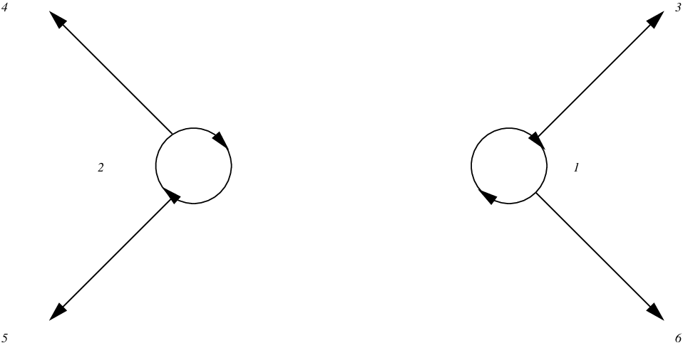
which solves the RHP depicted in Figure 4.

Refer to caption
Figure 4. The model RHP near z=+1z=+1 which can be solved explicitly using Hankel functions

More precisely, the function PB​ER​H​(ζ)P_{BE}^{RH}(\zeta) possesses the following analytic properties.

  • •

    PB​ER​H​(ζ)P_{BE}^{RH}(\zeta) is analytic for ζ∈ℂ\{arg​ζ=−π,−π6,π6}\zeta\in\mathbb{C}\backslash\{\textnormal{arg}\ \zeta=-\pi,-\frac{\pi}{6},\frac{\pi}{6}\}

  • •

    The following jumps hold

    (PB​ER​H​(ζ))+\displaystyle\big(P_{BE}^{RH}(\zeta)\big)_{+} =\displaystyle= (PB​ER​H​(ζ))−​(10−i1),arg​ζ=π6\displaystyle\big(P_{BE}^{RH}(\zeta)\big)_{-}\begin{pmatrix}1&0\\ -i&1\\ \end{pmatrix},\hskip 28.45274pt\textnormal{arg}\ \zeta=\frac{\pi}{6}
    (PB​ER​H​(ζ))+\displaystyle\big(P_{BE}^{RH}(\zeta)\big)_{+} =\displaystyle= (PB​ER​H​(ζ))−​(1−i01),arg​ζ=−π6\displaystyle\big(P_{BE}^{RH}(\zeta)\big)_{-}\begin{pmatrix}1&-i\\ 0&1\\ \end{pmatrix},\hskip 28.45274pt\textnormal{arg}\ \zeta=-\frac{\pi}{6}

    And for the jump on the line arg​ζ=π\textnormal{arg}\ \zeta=\pi we notice that the monodromy relations imply

    H0(2)​(ζ+)\displaystyle H_{0}^{(2)}\big(\sqrt{\zeta}_{+}\big) =\displaystyle= H0(2)​(ζ−​eπ​i)=H0(1)​(ζ−)+2​H0(2)​(ζ−)\displaystyle H_{0}^{(2)}\big(\sqrt{\zeta}_{-}e^{\pi i}\big)=H_{0}^{(1)}\big(\sqrt{\zeta}_{-}\big)+2H_{0}^{(2)}\big(\sqrt{\zeta}_{-}\big)
    (H0(2))′​(ζ+)\displaystyle\big(H_{0}^{(2)}\big)^{\prime}\big(\sqrt{\zeta}_{+}\big) =\displaystyle= e−i​π​(H0(1))′​(ζ−)+2​e−i​π​(H0(2))′​(ζ−)\displaystyle e^{-i\pi}\big(H_{0}^{(1)}\big)^{\prime}\big(\sqrt{\zeta}_{-}\big)+2e^{-i\pi}\big(H_{0}^{(2)}\big)^{\prime}\big(\sqrt{\zeta}_{-}\big)

    and

    H0(1)​(ζ+)\displaystyle H_{0}^{(1)}\big(\sqrt{\zeta}_{+}\big) =\displaystyle= H0(1)​(ζ−​eπ​i)=−H0(2)​(ζ−)\displaystyle H_{0}^{(1)}\big(\sqrt{\zeta}_{-}e^{\pi i}\big)=-H_{0}^{(2)}\big(\sqrt{\zeta}_{-}\big)
    (H0(1))′​(ζ+)\displaystyle\big(H_{0}^{(1)}\big)^{\prime}\big(\sqrt{\zeta}_{+}\big) =\displaystyle= (H0(2))′​(ζ−).\displaystyle\big(H_{0}^{(2)}\big)^{\prime}\big(\sqrt{\zeta}_{-}\big).

    Therefore

    (PB​E​(ζ))+=(PB​E​(ζ))−​ei​π4​σ3​(2−110)​e−i​π4​σ3=(PB​E​(ζ))−​(2−i−i0)\big(P_{BE}(\zeta)\big)_{+}=\big(P_{BE}(\zeta)\big)_{-}e^{i\frac{\pi}{4}\sigma_{3}}\begin{pmatrix}2&-1\\ 1&0\\ \end{pmatrix}e^{-i\frac{\pi}{4}\sigma_{3}}=\big(P_{BE}(\zeta)\big)_{-}\begin{pmatrix}2&-i\\ -i&0\\ \end{pmatrix}

    and hence

    (PB​ER​H​(ζ))+=(PB​ER​H​(ζ))−​(0−i−i0),arg​ζ=π,\big(P_{BE}^{RH}(\zeta)\big)_{+}=\big(P_{BE}^{RH}(\zeta)\big)_{-}\begin{pmatrix}0&-i\\ -i&0\\ \end{pmatrix},\ \ \ \textnormal{arg}\ \zeta=\pi,
  • •

    In order to determine the behavior of PB​ER​H​(ζ)P_{BE}^{RH}(\zeta) at infinity we make the following observations. First let arg​ζ∈(π6,π)\textnormal{arg}\ \zeta\in(\frac{\pi}{6},\pi) and consider

    e−i​ζ​σ3​(10−i1)​ei​ζ​σ3=(10−i​e2​i​ζ1).e^{-i\sqrt{\zeta}\sigma_{3}}\begin{pmatrix}1&0\\ -i&1\\ \end{pmatrix}e^{i\sqrt{\zeta}\sigma_{3}}=\begin{pmatrix}1&0\\ -ie^{2i\sqrt{\zeta}}&1\end{pmatrix}.

    Observe that Re​(i​ζ)<0\textnormal{Re}\big(i\sqrt{\zeta}\big)<0, hence the given product approaches the identity exponentially fast as ζ→∞\zeta\rightarrow\infty. Secondly for arg​ζ∈(−π,−π6)\textnormal{arg}\ \zeta\in(-\pi,-\frac{\pi}{6})

    e−i​ζ​σ3​(1i01)​ei​ζ​σ3=(1i​e−2​i​ζ01)e^{-i\sqrt{\zeta}\sigma_{3}}\begin{pmatrix}1&i\\ 0&1\\ \end{pmatrix}e^{i\sqrt{\zeta}\sigma_{3}}=\begin{pmatrix}1&ie^{-2i\sqrt{\zeta}}\\ 0&1\\ \end{pmatrix}

    and in this situation Re​(−i​ζ)<0\textnormal{Re}\big(-i\sqrt{\zeta}\big)<0, so again the product approaches the identity exponentially fast as ζ→∞\zeta\rightarrow\infty. Both cases together with the previously stated asymptotics for PB​E​(ζ)P_{BE}(\zeta) imply therefore

    (9.5) PB​ER​H​(ζ)\displaystyle P_{BE}^{RH}(\zeta) =\displaystyle= 2πζ−σ3/4ei​π4(11−11)[I+i8​ζ(−1−221)+3128​ζ(1−4−41)\displaystyle\sqrt{\frac{2}{\pi}}\zeta^{-\sigma_{3}/4}e^{i\frac{\pi}{4}}\begin{pmatrix}1&1\\ -1&1\\ \end{pmatrix}\bigg[I+\frac{i}{8\sqrt{\zeta}}\begin{pmatrix}-1&-2\\ 2&1\\ \end{pmatrix}+\frac{3}{128\zeta}\begin{pmatrix}1&-4\\ -4&1\\ \end{pmatrix}
    +15​i1024​ζ3/2(16−6−1)+O(ζ−2)]e−i​ζ​σ3,\displaystyle+\frac{15i}{1024\zeta^{3/2}}\begin{pmatrix}1&6\\ -6&-1\\ \end{pmatrix}+O\big(\zeta^{-2}\big)\bigg]e^{-i\sqrt{\zeta}\sigma_{3}},

    as ζ→∞\zeta\rightarrow\infty in a whole neighborhood of infinity.

The model function PB​ER​H​(ζ)P_{BE}^{RH}(\zeta) will now be used to construct the parametrix to the solution of the original XX-RHP in a neighborhood of z=+1z=+1. We proceed in two steps. First define

(9.6) ζ⁡(z)=−s6​g2​(z),|z−1|<r,−π<arg​ζ≤π\zeta(z)=-s^{6}g^{2}(z),\ \ |z-1|<r,\ -\pi<\textnormal{arg}\ \zeta\leq\pi

or respectively

ζ⁡(z)=−i​s3​g​(z)=4​s33​z2−1​(z2+12+3​x4​s2).\sqrt{\zeta(z)}=-is^{3}g(z)=\frac{4s^{3}}{3}\sqrt{z^{2}-1}\bigg(z^{2}+\frac{1}{2}+\frac{3x}{4s^{2}}\bigg).

This change of variables is indeed locally conformal, since

ζ⁡(z)=32​s69​(32+3​x4​s2)2​(z−1)​(1+O⁡(z−1)),|z−1|<r\zeta(z)=\frac{32s^{6}}{9}\bigg(\frac{3}{2}+\frac{3x}{4s^{2}}\bigg)^{2}(z-1)\big(1+O(z-1)\big),\ \ |z-1|<r

and it enables us to define the right parametrix U⁡(z)U(z) near z=+1z=+1 by the formula:

(9.7) U⁡(z)=Br​(z)​σ32​π2​e−i​π4​PB​ER​H​(ζ⁡(z))​es3​g​(z)​σ3,|z−1|<rU(z)=B_{r}(z)\frac{\sigma_{3}}{2}\sqrt{\frac{\pi}{2}}e^{-i\frac{\pi}{4}}P_{BE}^{RH}\big(\zeta(z)\big)e^{s^{3}g(z)\sigma_{3}},\ \ \ |z-1|<r

with ζ⁡(z)\zeta(z) as in (9.6) and the matrix multiplier

(9.8) Br​(z)=(111−1)​(ζ⁡(z)​z+1z−1)σ3/4,Br​(1)=(111−1)​(8​s33​(32+3​x4​s2))σ3/2.B_{r}(z)=\begin{pmatrix}1&1\\ 1&-1\\ \end{pmatrix}\bigg(\zeta(z)\frac{z+1}{z-1}\bigg)^{\sigma_{3}/4},\ \ B_{r}(1)=\begin{pmatrix}1&1\\ 1&-1\\ \end{pmatrix}\Bigg(\frac{8s^{3}}{3}\bigg(\frac{3}{2}+\frac{3x}{4s^{2}}\bigg)\Bigg)^{\sigma_{3}/2}.

By construction, in particular since Br​(z)B_{r}(z) is analytic in a neighborhood of z=+1z=+1, the parametrix U⁡(z)U(z) has jumps along the curves depicted in Figure 5, and we can always locally match the latter curves with the jump curves of the original RHP. Also these jumps are described by the same Stokes matrices as in the original TT-RHP. Furthermore, and we will elaborate this in full detail very soon, the singular behavior of U⁡(z)U(z) at the endpoint z=+1z=+1 matches the singular behavior of T⁡(z)T(z):

(9.9) U⁡(z)=O⁡(ln⁡(z−1)),|z−1|<r.U(z)=O\big(\ln(z-1)\big),\ \ |z-1|<r.

Hence the ratio of T⁡(z)T(z) with U⁡(z)U(z) is locally analytic, i.e.

(9.10) T⁡(z)=Nr​(z)​U​(z),|z−1|<r<12.T(z)=N_{r}(z)U(z),\ \ |z-1|<r<\frac{1}{2}.
Refer to caption
Figure 5. Transformation of parametrix jumps to original jumps

Let us explain the role of the left multiplier Br​(z)B_{r}(z) in the definition (9.7). Observe that

Br(z)ζ(z)−σ3/412(111−1)=M(z).B_{r}(z)\zeta(z)^{-\sigma_{3}/4}\frac{1}{2}\begin{pmatrix}1&1\\ 1&-1\\ \end{pmatrix}=M(z).

This relation together with the asymptotic equation (9.5) implies that,

(9.11) U⁡(z)\displaystyle U(z) =\displaystyle= (111−1)β(z)σ312(111−1)[I+i8​ζ(−1−221)+3128​ζ(1−4−41)\displaystyle\begin{pmatrix}1&1\\ 1&-1\\ \end{pmatrix}\beta(z)^{\sigma_{3}}\frac{1}{2}\begin{pmatrix}1&1\\ 1&-1\\ \end{pmatrix}\bigg[I+\frac{i}{8\sqrt{\zeta}}\begin{pmatrix}-1&-2\\ 2&1\\ \end{pmatrix}+\frac{3}{128\zeta}\begin{pmatrix}1&-4\\ -4&1\\ \end{pmatrix}
+15​i1024​ζ3/2(16−6−1)+O(ζ−2)]12(111−1)β(z)−σ3(111−1)M(z)\displaystyle+\frac{15i}{1024\zeta^{3/2}}\begin{pmatrix}1&6\\ -6&-1\\ \end{pmatrix}+O\big(\zeta^{-2}\big)\bigg]\frac{1}{2}\begin{pmatrix}1&1\\ 1&-1\\ \end{pmatrix}\beta(z)^{-\sigma_{3}}\begin{pmatrix}1&1\\ 1&-1\\ \end{pmatrix}M(z)
=\displaystyle= [I+i16​ζ(β2−3​β−2−(β2+3​β−2)β2+3​β−2−(β2−3​β−2))+3128​ζ(1−4−41)\displaystyle\bigg[I+\frac{i}{16\sqrt{\zeta}}\begin{pmatrix}\beta^{2}-3\beta^{-2}&-(\beta^{2}+3\beta^{-2})\\ \beta^{2}+3\beta^{-2}&-(\beta^{2}-3\beta^{-2})\\ \end{pmatrix}+\frac{3}{128\zeta}\begin{pmatrix}1&-4\\ -4&1\\ \end{pmatrix}
+15​i2048​ζ3/2(−(5​β2−7​β−2)5​β2+7​β−2−(5​β2+7​β−2)5​β2−7​β−2)+O(ζ−2)]M(z)\displaystyle+\frac{15i}{2048\zeta^{3/2}}\begin{pmatrix}-(5\beta^{2}-7\beta^{-2})&5\beta^{2}+7\beta^{-2}\\ -(5\beta^{2}+7\beta^{-2})&5\beta^{2}-7\beta^{-2}\\ \end{pmatrix}+O\big(\zeta^{-2}\big)\bigg]M(z)

as s→∞s\rightarrow\infty and 0<r1≤|z−1|≤r2<10<r_{1}\leq|z-1|\leq r_{2}<1 (so |ζ|→∞|\zeta|\rightarrow\infty). Since the function ζ⁡(z)\zeta(z) is of order O⁡(s6)O\big(s^{6}\big) on the latter annulus and β⁡(z)\beta(z) is bounded, equation (9.11) yields the matching relation between the model functions U⁡(z)U(z) and M⁡(z)M(z),

U⁡(z)=(I+o⁡(1))​M​(z),s→∞, 0<r1≤|z−1|≤r2<1U(z)=\big(I+o(1)\big)M(z),\hskip 14.22636pts\rightarrow\infty,\ \ 0<r_{1}\leq|z-1|\leq r_{2}<1

which is crucial for the successful implementation of the nonlinear steepest descent method as we shall see after the next subsection. This is the reason for chosing the left multiplier Br​(z)B_{r}(z) in (9.7) in the form (9.8).

10. Construction of a parametrix at the edge point z=−1z=-1

The model RHP near the other endpoint z=−1z=-1 can be introduced in a similar way as we did it in the last section. First we consider on the punctured plane ζ∈ℂ\{0}\zeta\in\mathbb{C}\backslash\{0\}

P~B​E​(ζ)=(e−i​3​π2​ζ​(H0(1))′​(e−i​π2​ζ)−ζ​(H0(2))′​(e−i​π2​ζ)−ei​π2​H0(1)​(e−i​π2​ζ)H0(2)​(e−i​π2​ζ)), 0<arg​ζ≤2​π\tilde{P}_{BE}(\zeta)=\begin{pmatrix}e^{-i\frac{3\pi}{2}}\sqrt{\zeta}\Big(H_{0}^{(1)}\Big)^{\prime}\big(e^{-i\frac{\pi}{2}}\sqrt{\zeta}\big)&-\sqrt{\zeta}\Big(H_{0}^{(2)}\Big)^{\prime}\big(e^{-i\frac{\pi}{2}}\sqrt{\zeta}\big)\\ -e^{i\frac{\pi}{2}}H_{0}^{(1)}\big(e^{-i\frac{\pi}{2}}\sqrt{\zeta}\big)&H_{0}^{(2)}\big(e^{-i\frac{\pi}{2}}\sqrt{\zeta}\big)\\ \end{pmatrix},\ \ \ 0<\textnormal{arg}\ \zeta\leq 2\pi

satisfying

P~B​E​(ζ)\displaystyle\tilde{P}_{BE}(\zeta) =\displaystyle= 2πζσ3/4(−1−1−ii)[I+18​ζ(−12−21)+3128​ζ(−1−4−4−1)\displaystyle\sqrt{\frac{2}{\pi}}\zeta^{\sigma_{3}/4}\begin{pmatrix}-1&-1\\ -i&i\\ \end{pmatrix}\bigg[I+\frac{1}{8\sqrt{\zeta}}\begin{pmatrix}-1&2\\ -2&1\\ \end{pmatrix}+\frac{3}{128\zeta}\begin{pmatrix}-1&-4\\ -4&-1\\ \end{pmatrix}
+151024​ζ3/2(−16−61)+O(ζ−2)]eζ​σ3\displaystyle+\frac{15}{1024\zeta^{3/2}}\begin{pmatrix}-1&6\\ -6&1\\ \end{pmatrix}+O\big(\zeta^{-2}\big)\bigg]e^{\sqrt{\zeta}\sigma_{3}}

as ζ→∞\zeta\rightarrow\infty and 0<arg​ζ≤2​π0<\textnormal{arg}\ \zeta\leq 2\pi. Next, instead of (9.4), define

(10.1) P~B​ER​H​(ζ)={P~B​E​(ζ)​(10−i1),arg ζ∈(0,5​π6),P~B​E​(ζ)​(1i01),arg ζ∈(7​π6,2​π),P~B​E​(ζ),arg ζ∈(5​π6,7​π6).\tilde{P}_{BE}^{RH}(\zeta)=\left\{\begin{array}[]{ll}\tilde{P}_{BE}(\zeta)\begin{pmatrix}1&0\\ -i&1\\ \end{pmatrix},&\hbox{arg $\zeta\in(0,\frac{5\pi}{6})$,}\\ \tilde{P}_{BE}(\zeta)\begin{pmatrix}1&i\\ 0&1\\ \end{pmatrix},&\hbox{arg $\zeta\in(\frac{7\pi}{6},2\pi)$,}\\ \tilde{P}_{BE}(\zeta),&\hbox{arg $\zeta\in(\frac{5\pi}{6},\frac{7\pi}{6})$.}\end{array}\right.

which solves the model RHP of Figure 6. More precisely, the function P~B​ER​H​(ζ)\tilde{P}_{BE}^{RH}(\zeta) has the following analytic properties

Refer to caption
Figure 6. The model RHP near z=−1z=-1 which can be solved explicitly using Hankel functions
  • •

    P~B​ER​H​(ζ)\tilde{P}_{BE}^{RH}(\zeta) is analytic for ζ∈ℂ\{arg​ζ=5​π6,7​π6,2​π}\zeta\in\mathbb{C}\backslash\{\textnormal{arg}\ \zeta=\frac{5\pi}{6},\frac{7\pi}{6},2\pi\}

  • •

    We have the following jumps on the contour depicted in Figure 6

    (P~B​ER​H​(ζ))+\displaystyle\big(\tilde{P}_{BE}^{RH}(\zeta)\big)_{+} =\displaystyle= (P~B​ER​H​(ζ))−​(10i1),arg​ζ=5​π6\displaystyle\big(\tilde{P}_{BE}^{RH}(\zeta)\big)_{-}\begin{pmatrix}1&0\\ i&1\\ \end{pmatrix},\ \ \ \textnormal{arg}\ \zeta=\frac{5\pi}{6}
    (P~B​ER​H​(ζ))+\displaystyle\big(\tilde{P}_{BE}^{RH}(\zeta)\big)_{+} =\displaystyle= (P~B​ER​H​(ζ))−​(1i01),arg​ζ=7​π6\displaystyle\big(\tilde{P}_{BE}^{RH}(\zeta)\big)_{-}\begin{pmatrix}1&i\\ 0&1\\ \end{pmatrix},\ \ \ \textnormal{arg}\ \zeta=\frac{7\pi}{6}

    and on the line segment arg​ζ=2​π\textnormal{arg}\ \zeta=2\pi

    H0(1)​(e−i​π2​ζ+)\displaystyle H_{0}^{(1)}\big(e^{-i\frac{\pi}{2}}\sqrt{\zeta}_{+}\big) =\displaystyle= H0(1)​(e−i​π2​ζ−​e−i​π)=H0(2)​(e−i​π2​ζ−)+2​H0(1)​(e−i​π2​ζ−)\displaystyle H_{0}^{(1)}\big(e^{-i\frac{\pi}{2}}\sqrt{\zeta}_{-}e^{-i\pi}\big)=H_{0}^{(2)}\big(e^{-i\frac{\pi}{2}}\sqrt{\zeta}_{-}\big)+2H_{0}^{(1)}\big(e^{-i\frac{\pi}{2}}\sqrt{\zeta}_{-}\big)
    (H0(1))′​(e−i​π2​ζ+)\displaystyle\big(H_{0}^{(1)}\big)^{\prime}\big(e^{-i\frac{\pi}{2}}\sqrt{\zeta}_{+}\big) =\displaystyle= ei​π​(H0(2))′​(e−i​π2​ζ−)+2​ei​π​(H0(1))′​(e−i​π2​ζ−)\displaystyle e^{i\pi}\big(H_{0}^{(2)}\big)^{\prime}\big(e^{-i\frac{\pi}{2}}\sqrt{\zeta}_{-}\big)+2e^{i\pi}\big(H_{0}^{(1)}\big)^{\prime}\big(e^{-i\frac{\pi}{2}}\sqrt{\zeta}_{-}\big)

    as well as

    H0(2)​(e−i​π2​ζ+)\displaystyle H_{0}^{(2)}\big(e^{-i\frac{\pi}{2}}\sqrt{\zeta}_{+}\big) =\displaystyle= H0(2)​(e−i​π2​ζ−​e−i​π)=−H0(1)​(e−i​π2​ζ−)\displaystyle H_{0}^{(2)}\big(e^{-i\frac{\pi}{2}}\sqrt{\zeta}_{-}e^{-i\pi}\big)=-H_{0}^{(1)}\big(e^{-i\frac{\pi}{2}}\sqrt{\zeta}_{-}\big)
    (H0(2))′​(e−i​π2​ζ+)\displaystyle\big(H_{0}^{(2)}\big)^{\prime}\big(e^{-i\frac{\pi}{2}}\sqrt{\zeta}_{+}\big) =\displaystyle= (H0(1))′​(e−i​π2​ζ−)\displaystyle\big(H_{0}^{(1)}\big)^{\prime}\big(e^{-i\frac{\pi}{2}}\sqrt{\zeta}_{-}\big)

    hence

    (P~B​ER​H​(ζ))+=(P~B​ER​H​(ζ))−​(0−i−i0),arg​ζ=2​π.\big(\tilde{P}_{BE}^{RH}(\zeta)\big)_{+}=\big(\tilde{P}_{BE}^{RH}(\zeta)\big)_{-}\begin{pmatrix}0&-i\\ -i&0\\ \end{pmatrix},\ \ \ \textnormal{arg}\ \zeta=2\pi.
  • •

    A similar argument as given in the construction of PB​ER​H​(ζ)P_{BE}^{RH}(\zeta) implies

    (10.2) P~B​ER​H​(ζ)\displaystyle\tilde{P}_{BE}^{RH}(\zeta) =\displaystyle= 2πζσ3/4(−1−1−ii)[I+18​ζ(−12−21)+3128​ζ(−1−4−4−1)\displaystyle\sqrt{\frac{2}{\pi}}\zeta^{\sigma_{3}/4}\begin{pmatrix}-1&-1\\ -i&i\\ \end{pmatrix}\bigg[I+\frac{1}{8\sqrt{\zeta}}\begin{pmatrix}-1&2\\ -2&1\\ \end{pmatrix}+\frac{3}{128\zeta}\begin{pmatrix}-1&-4\\ -4&-1\\ \end{pmatrix}
    +151024​ζ3/2(−16−61)+O(ζ−2)]eζ​σ3\displaystyle+\frac{15}{1024\zeta^{3/2}}\begin{pmatrix}-1&6\\ -6&1\\ \end{pmatrix}+O\big(\zeta^{-2}\big)\bigg]e^{\sqrt{\zeta}\sigma_{3}}

    as ζ→∞\zeta\rightarrow\infty, valid in a full neighborhood of infinity.

Again we use the model function P~B​ER​H​(ζ)\tilde{P}_{BE}^{RH}(\zeta) in the construction of the parametrix to the solution of the original XX-RHP near z=−1z=-1. Instead of (9.6)

(10.3) ζ⁡(z)=s6​g2​(z),|z+1|<r, 0<arg​ζ≤2​π\zeta(z)=s^{6}g^{2}(z),\ \ |z+1|<r,\ 0<\textnormal{arg}\ \zeta\leq 2\pi

or equivalently

ζ⁡(z)=−s3​g​(z)=−4​i​s33​z2−1​(z2+12+3​x4​s2).\sqrt{\zeta(z)}=-s^{3}g(z)=-\frac{4is^{3}}{3}\sqrt{z^{2}-1}\bigg(z^{2}+\frac{1}{2}+\frac{3x}{4s^{2}}\bigg).

This change of the independent variable is locally conformal

ζ⁡(z)=32​s69​(32+3​x4​s2)2​(z+1)​(1+O⁡(z+1)),|z+1|<r\zeta(z)=\frac{32s^{6}}{9}\bigg(\frac{3}{2}+\frac{3x}{4s^{2}}\bigg)^{2}(z+1)\big(1+O(z+1)\big),\ \ |z+1|<r

and allows us to define the left parametrix V⁡(z)V(z) near z=−1z=-1 by the formula:

(10.4) V⁡(z)=Bl​(z)​12​(−100i)​π2​P~B​ER​H​(ζ⁡(z))​es3​g​(z)​σ3,|z+1|<rV(z)=B_{l}(z)\frac{1}{2}\begin{pmatrix}-1&0\\ 0&i\\ \end{pmatrix}\sqrt{\frac{\pi}{2}}\tilde{P}_{BE}^{RH}\big(\zeta(z)\big)e^{s^{3}g(z)\sigma_{3}},\ \ |z+1|<r

with the matrix multiplier

(10.5) Bl(z)=(111−1)(ζ(z)z−1z+1)−σ3/4,Bl(−1)=(111−1)(8​i​s33(32+3​x4​s2))−σ3/2.B_{l}(z)=\begin{pmatrix}1&1\\ 1&-1\\ \end{pmatrix}\bigg(\zeta(z)\frac{z-1}{z+1}\bigg)^{-\sigma_{3}/4},\ \ B_{l}(-1)=\begin{pmatrix}1&1\\ 1&-1\\ \end{pmatrix}\Bigg(\frac{8is^{3}}{3}\bigg(\frac{3}{2}+\frac{3x}{4s^{2}}\bigg)\Bigg)^{-\sigma_{3}/2}.

Similar to the situation in the last section, V⁡(z)V(z) has jumps on the contour depicted in Figure 7 which are described by the same Stokes matrices as in the original TT-RHP.

Refer to caption
Figure 7. Transformation of parametrix jumps to original jumps

Also here, as we shall see in detail in the section 13, the singular behavior at z=−1z=-1 matches:

(10.6) V⁡(z)=O⁡(ln⁡(z+1)),|z+1|<rV(z)=O\big(\ln(z+1)\big),\ \ |z+1|<r

Hence the ratio of parametrix V⁡(z)V(z) with T⁡(z)T(z) is locally analytic

T⁡(z)=Nl​(z)​V​(z),|z+1|<r<12T(z)=N_{l}(z)V(z),\ \ |z+1|<r<\frac{1}{2}

and the left multiplier (10.5) in (10.4) provides us with the following asymptotic matchup between V⁡(z)V(z) and M⁡(z)M(z):

(10.7) V⁡(z)\displaystyle V(z) =\displaystyle= (111−1)β(z)σ312(111−1)[I+18​ζ(−12−21)+3128​ζ(−1−4−4−1)\displaystyle\begin{pmatrix}1&1\\ 1&-1\\ \end{pmatrix}\beta(z)^{\sigma_{3}}\frac{1}{2}\begin{pmatrix}1&1\\ 1&-1\\ \end{pmatrix}\bigg[I+\frac{1}{8\sqrt{\zeta}}\begin{pmatrix}-1&2\\ -2&1\\ \end{pmatrix}+\frac{3}{128\zeta}\begin{pmatrix}-1&-4\\ -4&-1\\ \end{pmatrix}
+151024​ζ3/2(−16−61)+O(ζ−2)]12(111−1)β(z)−σ3(111−1)M(z)\displaystyle+\frac{15}{1024\zeta^{3/2}}\begin{pmatrix}-1&6\\ -6&1\\ \end{pmatrix}+O\big(\zeta^{-2}\big)\bigg]\frac{1}{2}\begin{pmatrix}1&1\\ 1&-1\\ \end{pmatrix}\beta(z)^{-\sigma_{3}}\begin{pmatrix}1&1\\ 1&-1\\ \end{pmatrix}M(z)
=\displaystyle= [I+116​ζ(β−2−3​β2β−2+3​β2−(β−2+3​β2)−(β−2−3​β2))+3128​ζ(−1−4−4−1)\displaystyle\bigg[I+\frac{1}{16\sqrt{\zeta}}\begin{pmatrix}\beta^{-2}-3\beta^{2}&\beta^{-2}+3\beta^{2}\\ -(\beta^{-2}+3\beta^{2})&-(\beta^{-2}-3\beta^{2})\\ \end{pmatrix}+\frac{3}{128\zeta}\begin{pmatrix}-1&-4\\ -4&-1\\ \end{pmatrix}
+152048​ζ3/2(5​β−2−7​β25​β−2+7​β2−(5​β−2+7​β2)−(5​β−2−7​β2))+O(ζ−2)]M(z)\displaystyle+\frac{15}{2048\zeta^{3/2}}\begin{pmatrix}5\beta^{-2}-7\beta^{2}&5\beta^{-2}+7\beta^{2}\\ -(5\beta^{-2}+7\beta^{2})&-(5\beta^{-2}-7\beta^{2})\\ \end{pmatrix}+O\big(\zeta^{-2}\big)\bigg]M(z)

as s→∞s\rightarrow\infty and 0<r1≤|z+1|≤r2<10<r_{1}\leq|z+1|\leq r_{2}<1, thus

V⁡(z)=(I+o⁡(1))​M​(z),s→∞, 0<r1≤|z+1|≤r2<1.V(z)=\big(I+o(1)\big)M(z),\hskip 14.22636pts\rightarrow\infty,\ \ 0<r_{1}\leq|z+1|\leq r_{2}<1.

At this point we can use the model functions M⁡(z),U⁡(z)M(z),U(z) and V⁡(z)V(z) to employ the final transformation.

11. Third and final transformation of the RHP

In this final transformation we put

(11.1) R⁡(z)=T⁡(z)​{(U⁡(z))−1,|z−1|<r,(V⁡(z))−1,|z+1|<r,(M⁡(z))−1,|z∓1|>rR(z)=T(z)\left\{\begin{array}[]{ll}\big(U(z)\big)^{-1},&\hbox{$|z-1|<r$,}\\ \big(V(z)\big)^{-1},&\hbox{$|z+1|<r$,}\\ \big(M(z)\big)^{-1},&\hbox{$|z\mp 1|>r$}\end{array}\right.

where 0<r<140<r<\frac{1}{4} remains fixed. With CrC_{r} and ClC_{l} denoting the clockwise oriented circles shown in Figure 8, the ratio-function R⁡(z)R(z) solves the following RHP

Refer to caption
Figure 8. The jump graph for the ratio-function R⁡(z)R(z)
  • •

    R⁡(z)R(z) is anlytic for z∈ℂ\{Cr∪Cl∪⋃kγk}z\in\mathbb{C}\backslash\big\{C_{r}\cup C_{l}\cup\bigcup_{k}\gamma_{k}\big\}

  • •

    Along the infinite branches γk\gamma_{k}

    R+​(z)=R−​(z)​M​(z)​e−s3​g​(z)​σ3​Sk​es3​g​(z)​σ3​(M⁡(z))−1,z∈γk,R_{+}(z)=R_{-}(z)M(z)e^{-s^{3}g(z)\sigma_{3}}S_{k}e^{s^{3}g(z)\sigma_{3}}\big(M(z)\big)^{-1},\ \ z\in\gamma_{k},

    and on the clockwise oriented circles Cr,lC_{r,l}

    R+​(z)\displaystyle R_{+}(z) =\displaystyle= R−​(z)​U​(z)​(M⁡(z))−1,z∈Cr\displaystyle R_{-}(z)U(z)\big(M(z)\big)^{-1},\ z\in C_{r}
    R+​(z)\displaystyle R_{+}(z) =\displaystyle= R−​(z)​V​(z)​(M⁡(z))−1,z∈Cl\displaystyle R_{-}(z)V(z)\big(M(z)\big)^{-1},\ z\in C_{l}
  • •

    R⁡(z)R(z) is analytic at z=±1z=\pm 1. This observation follows from (9.9) and (10.6), which will be proved in section 13.

  • •

    In a neigborhood of infinity, we have R⁡(z)→IR(z)\rightarrow I

We emphasize that, by construction, the function R⁡(z)R(z) has no jumps inside of CrC_{r} and ClC_{l} and across the line segment in between them. In order to apply the Deift-Zhou nonlinear steepest descent method for the ratio-RHP, all its jump matrices have to be close to the unit matrix, as s→∞s\rightarrow\infty, see [14]. Due to the triangularity of all Stokes matrices SkS_{k}, the jump matrices corresponding to the infinite parts ⋃kγk\bigcup_{k}\gamma_{k} of the RR-jump contour are in fact exponentially close to the unit matrix

(11.2) ‖M​e−s3​g​(⋅)​σ3​Sk​es3​g​(⋅)​σ3​(M)−1−I‖L2∩L∞​(γk)≤c1​e−c2​s3​|z∓1|\|Me^{-s^{3}g(\cdot)\sigma_{3}}S_{k}e^{s^{3}g(\cdot)\sigma_{3}}\big(M\big)^{-1}-I\|_{L^{2}\cap L^{\infty}(\gamma_{k})}\leq c_{1}e^{-c_{2}s^{3}|z\mp 1|}

emanating from Cr,lC_{r,l} as s→∞s\rightarrow\infty with constants ci>0c_{i}>0 whose values are not important. Moreover, by virtue of (9.11), U⁡(z)​(M⁡(z))−1U(z)\big(M(z)\big)^{-1} approaches the unit matrix as s→∞s\rightarrow\infty

(11.3) ‖U​(M)−1−I‖L2∩L∞​(Cr)≤c3​s−3\|U\big(M\big)^{-1}-I\|_{L^{2}\cap L^{\infty}(C_{r})}\leq c_{3}s^{-3}

and from (10.7), also V⁡(z)​(M⁡(z))−1V(z)\big(M(z)\big)^{-1}

(11.4) ‖V​(M)−1−I‖L2∩L∞​(Cl)≤c4​s−3,s→∞.\|V\big(M\big)^{-1}-I\|_{L^{2}\cap L^{\infty}(C_{l})}\leq c_{4}s^{-3},\ s\rightarrow\infty.

All together, with GRG_{R} denoting the jump matrix in the latter ratio-RHP and ΣR\Sigma_{R} the underlying contour

(11.5) ‖GR−I‖L2∩L∞​(ΣR)≤c​s−3,s→∞\|G_{R}-I\|_{L^{2}\cap L^{\infty}(\Sigma_{R})}\leq cs^{-3},\ \ s\rightarrow\infty

uniformly on any compact subset of the set (1.15). The latter estimation enables us to solve the ratio-RHP iteratively.

12. Solution of the RHP for R⁡(z)R(z) via iteration

The RHP for the function R⁡(z)R(z),

  • •

    R⁡(z)R(z) is analytic for z∈ℂ\ΣRz\in\mathbb{C}\backslash\Sigma_{R}

  • •

    Along the contour depicted in Figure 8

    R+​(z)=R−​(z)​GR​(z),z∈ΣRR_{+}(z)=R_{-}(z)G_{R}(z),\ \ z\in\Sigma_{R}
  • •

    At infinity, R⁡(z)=I+O⁡(z−1),z→∞R(z)=I+O\big(z^{-1}\big),z\rightarrow\infty

is equivalent to the singular integral equation

(12.1) R−​(z)=I+12​π​i​∫ΣRR−​(w)​(GR​(w)−I)​d​ww−z−R_{-}(z)=I+\frac{1}{2\pi i}\int\limits_{\Sigma_{R}}R_{-}(w)\big(G_{R}(w)-I\big)\frac{dw}{w-z_{-}}

and by standard arguments (see [14]) we know that for sufficiently large ss the relevant integral operator is contracting and equation (12.1) can be solved iteratively in L2​(ΣR)L^{2}(\Sigma_{R}). Moreover, its unique solution satisfies

(12.2) ‖R−−I‖L2​(ΣR)≤c​s−3,s→∞.\|R_{-}-I\|_{L^{2}(\Sigma_{R})}\leq cs^{-3},\ \ s\rightarrow\infty.

It is now time to connect the latter information with (5.4) and (5.5) to determine the large ss asymptotics of det(I−KPII)\det(I-K_{\textnormal{PII}}) up to the constant term.

13. Asymptotics of lndet(I−KPII)\ln\det(I-K_{\textnormal{PII}}) - preliminary steps

Let us recall the transformations, which have been used in the asymptotical solution of the original YY-RHP

Y⁡(λ)↦X~​(λ)↦X⁡(λ)↦T⁡(z)↦R⁡(z).Y(\lambda)\mapsto\tilde{X}(\lambda)\mapsto X(\lambda)\mapsto T(z)\mapsto R(z).

Thus, in order to determine lndet(I−KPII)\ln\det(I-K_{\textnormal{PII}}) via Proposition 1 we need to connect Xˇ​(±s)\check{X}(\pm s) and Xˇ′​(±s)\check{X}^{\prime}(\pm s) to the values R⁡(±1)R(\pm 1) and R′​(±1)R^{\prime}(\pm 1) of the ratio-function. This can be done as follows: From (11.1) and (7.5) for |z−1|<r|z-1|<r

(13.1) R⁡(z)​U​(z)​e−s3​g​(z)​σ3=Xˇ​(z​s)​(1−12​π​ln⁡z−1z+101)​{I,λ∈Ω^1,S3​S4,λ∈Ω^3,S3​S4​S6,λ∈Ω^4,R(z)U(z)e^{-s^{3}g(z)\sigma_{3}}=\check{X}(zs)\begin{pmatrix}1&-\frac{1}{2\pi}\ln\frac{z-1}{z+1}\\ 0&1\\ \end{pmatrix}\left\{\begin{array}[]{ll}I,&\hbox{$\lambda\in\hat{\Omega}_{1}$,}\\ S_{3}S_{4},&\hbox{$\lambda\in\hat{\Omega}_{3}$,}\\ S_{3}S_{4}S_{6},&\hbox{$\lambda\in\hat{\Omega}_{4}$,}\end{array}\right.

and for |z+1|<r|z+1|<r

(13.2) R⁡(z)​V​(z)​e−s3​g​(z)​σ3=Xˇ​(z​s)​(1−12​π​ln⁡z−1z+101)​{I,λ∈Ω^1,S3,λ∈Ω^2,S3​S4,λ∈Ω^3.R(z)V(z)e^{-s^{3}g(z)\sigma_{3}}=\check{X}(zs)\begin{pmatrix}1&-\frac{1}{2\pi}\ln\frac{z-1}{z+1}\\ 0&1\\ \end{pmatrix}\left\{\begin{array}[]{ll}I,&\hbox{$\lambda\in\hat{\Omega}_{1}$,}\\ S_{3},&\hbox{$\lambda\in\hat{\Omega}_{2}$,}\\ S_{3}S_{4},&\hbox{$\lambda\in\hat{\Omega}_{3}$.}\end{array}\right.

This shows that the required values of Xˇ​(±s)\check{X}(\pm s) and Xˇ′​(±s)\check{X}^{\prime}(\pm s) can be determined via comparison in either (13.1) or (13.2), once we know the local expansions of U⁡(z)U(z), respectively V⁡(z)V(z) at z=±1z=\pm 1. Our starting point is (9.2)

(13.3) PB​ER​H​(ζ)\displaystyle P_{BE}^{RH}(\zeta) =\displaystyle= (a¯0+a¯12​ln⁡ζi⁡(a0+a12​ln⁡ζ)a¯1a1)\displaystyle\begin{pmatrix}\bar{a}_{0}+\frac{\bar{a}_{1}}{2}\ln\zeta&i(a_{0}+\frac{a_{1}}{2}\ln\zeta)\\ \bar{a}_{1}&a_{1}\end{pmatrix}
+ζ​(a¯2+a¯32​ln⁡ζi⁡(a2+a32​ln⁡ζ)2​a¯2+a¯3+a¯3​ln⁡ζ2​a2+a3+a3​ln⁡ζ)+O⁡(ζ2​ln⁡ζ),\displaystyle+\zeta\begin{pmatrix}\bar{a}_{2}+\frac{\bar{a}_{3}}{2}\ln\zeta&i(a_{2}+\frac{a_{3}}{2}\ln\zeta)\\ 2\bar{a}_{2}+\bar{a}_{3}+\bar{a}_{3}\ln\zeta&2a_{2}+a_{3}+a_{3}\ln\zeta\\ \end{pmatrix}+O\big(\zeta^{2}\ln\zeta),

as ζ→0\zeta\rightarrow 0 and −π6<arg​ζ<π6-\frac{\pi}{6}<\textnormal{arg}\ \zeta<\frac{\pi}{6}. The latter expansion together with the changes of variables ζ=ζ⁡(z)=−s6​g2​(z)\zeta=\zeta(z)=-s^{6}g^{2}(z) and λ=z​s\lambda=zs implies for −π6<arg​(λ−s)<π6-\frac{\pi}{6}<\textnormal{arg}\ (\lambda-s)<\frac{\pi}{6}

PB​ER​H​(ζ⁡(z))=Ω⁡(ln⁡(λ−s))+(λ−s)​Π​(ln⁡(λ−s))+O⁡((λ−s)2​ln⁡(λ−s)),λ→sP_{BE}^{RH}\big(\zeta(z)\big)=\Omega\big(\ln(\lambda-s)\big)+(\lambda-s)\Pi\big(\ln(\lambda-s)\big)+O\big((\lambda-s)^{2}\ln(\lambda-s)\big),\ \ \lambda\rightarrow s

with the matrix functions Ω=(Ωi​j)\Omega=(\Omega_{ij}) and Π=(Πi​j)\Pi=(\Pi_{ij}) being determined from (13.3). Now we combine the latter expansion with (9.7) and (11.1)

R⁡(z)​U​(z)​e−s3​g​(z)​σ3|z=λs=R⁡(z)​Br​(z)​σ32​π2​e−i​π4​PB​ER​H​(ζ⁡(z))|z=λs\displaystyle R(z)U(z)e^{-s^{3}g(z)\sigma_{3}}\Big|_{z=\frac{\lambda}{s}}=R(z)B_{r}(z)\frac{\sigma_{3}}{2}\sqrt{\frac{\pi}{2}}e^{-i\frac{\pi}{4}}P_{BE}^{RH}\big(\zeta(z)\big)\Big|_{z=\frac{\lambda}{s}}
=\displaystyle= R(1)Br(1)σ32π2e−i​π4Ω(ln(λ−s))+(λ−s){R(1)Br(1)\displaystyle R(1)B_{r}(1)\frac{\sigma_{3}}{2}\sqrt{\frac{\pi}{2}}e^{-i\frac{\pi}{4}}\Omega\big(\ln(\lambda-s)\big)+(\lambda-s)\bigg\{R(1)B_{r}(1)
×σ32π2e−i​π4Π(ln(λ−s))+(R′(1)Br(1)+R(1)Br′(1))σ32π2e−i​π4Ω⁡(ln⁡(λ−s))s}\displaystyle\times\frac{\sigma_{3}}{2}\sqrt{\frac{\pi}{2}}e^{-i\frac{\pi}{4}}\Pi\big(\ln(\lambda-s)\big)+\big(R^{\prime}(1)B_{r}(1)+R(1)B_{r}^{\prime}(1)\big)\frac{\sigma_{3}}{2}\sqrt{\frac{\pi}{2}}e^{-i\frac{\pi}{4}}\frac{\Omega\big(\ln(\lambda-s)\big)}{s}\bigg\}
+O⁡((λ−s)2​ln⁡(λ−s)),λ→s,−π6<arg​(λ−s)<π6\displaystyle+O\big((\lambda-s)^{2}\ln(\lambda-s)\big),\ \ \lambda\rightarrow s,\ \ -\frac{\pi}{6}<\textnormal{arg}\ (\lambda-s)<\frac{\pi}{6}

and similar identities hold for −π<arg​(λ−s)<−π6-\pi<\textnormal{arg}\ (\lambda-s)<-\frac{\pi}{6} and π6<arg​(λ−s)<π\frac{\pi}{6}<\textnormal{arg}\ (\lambda-s)<\pi, they differ from (13.3) only by right multiplication with a Stokes matrix (see (9.4)). On the other hand the right hand side in (13.1) implies for −π6<arg​(λ−s)<π6-\frac{\pi}{6}<\textnormal{arg}\ (\lambda-s)<\frac{\pi}{6}

T⁡(λs)​e−s3​g​(λs)​σ3=[Xˇ​(s)+(λ−s)​Xˇ′​(s)+O⁡((λ−s)2)]​(1−12​π​ln⁡λ−sλ+s01)​(10i1)\displaystyle T\Big(\frac{\lambda}{s}\Big)e^{-s^{3}g(\frac{\lambda}{s})\sigma_{3}}=\Big[\check{X}(s)+(\lambda-s)\check{X}^{\prime}(s)+O\big((\lambda-s)^{2}\big)\Big]\begin{pmatrix}1&-\frac{1}{2\pi}\ln\frac{\lambda-s}{\lambda+s}\\ 0&1\\ \end{pmatrix}\begin{pmatrix}1&0\\ i&1\\ \end{pmatrix}
=\displaystyle= [(Xˇ11​(s)12​π​ln⁡(2​s)​Xˇ11​(s)+Xˇ12​(s)Xˇ21​(s)12​π​ln⁡(2​s)​Xˇ21​(s)+Xˇ22​(s))\displaystyle\Bigg[\begin{pmatrix}\check{X}_{11}(s)&\frac{1}{2\pi}\ln(2s)\check{X}_{11}(s)+\check{X}_{12}(s)\\ \check{X}_{21}(s)&\frac{1}{2\pi}\ln(2s)\check{X}_{21}(s)+\check{X}_{22}(s)\\ \end{pmatrix}
+(λ−s)(Xˇ11′​(s)12​π​(ln⁡(2​s)​Xˇ11′​(s)+12​s​Xˇ11​(s))+Xˇ12′​(s)Xˇ21′​(s)12​π​(ln⁡(2​s)​Xˇ21′​(s)+12​s​Xˇ21​(s))+Xˇ22′​(s))]\displaystyle+(\lambda-s)\begin{pmatrix}\check{X}_{11}^{\prime}(s)&\frac{1}{2\pi}(\ln(2s)\check{X}_{11}^{\prime}(s)+\frac{1}{2s}\check{X}_{11}(s))+\check{X}_{12}^{\prime}(s)\\ \check{X}_{21}^{\prime}(s)&\frac{1}{2\pi}(\ln(2s)\check{X}_{21}^{\prime}(s)+\frac{1}{2s}\check{X}_{21}(s))+\check{X}_{22}^{\prime}(s)\\ \end{pmatrix}\Bigg]
×(1−i2​π​ln⁡(λ−s)−12​π​ln⁡(λ−s)i1)+O⁡((λ−s)2​ln⁡(λ−s)),λ→s\displaystyle\times\begin{pmatrix}1-\frac{i}{2\pi}\ln(\lambda-s)&-\frac{1}{2\pi}\ln(\lambda-s)\\ i&1\\ \end{pmatrix}+O\big((\lambda-s)^{2}\ln(\lambda-s)\big),\ \ \lambda\rightarrow s

and thus by comparison of the left hand side and right hand side in (13.1)

(13.4) Xˇ11​(s)=π2​e−i​π4​(R⁡(1)​Br​(1))11,Xˇ21​(s)=π2​e−i​π4​(R⁡(1)​Br​(1))21.\check{X}_{11}(s)=\sqrt{\frac{\pi}{2}}e^{-i\frac{\pi}{4}}\big(R(1)B_{r}(1)\big)_{11},\ \ \ \ \check{X}_{21}(s)=\sqrt{\frac{\pi}{2}}e^{-i\frac{\pi}{4}}\big(R(1)B_{r}(1)\big)_{21}.

Although (13.4) was derived from a comparison in the sector −π6<arg​(λ−s)<π6-\frac{\pi}{6}<\textnormal{arg}\ (\lambda-s)<\frac{\pi}{6}, the multiplication of (13.3) with the right Stokes matrix in the other sectors as well as the use of appropriate Stokes matrices in (4.1) show that (13.4) follows from comparison in a full neighborhood of λ=+s\lambda=+s. Comparing terms of O⁡((λ−s)​ln⁡(λ−s))O\big((\lambda-s)\ln(\lambda-s)\big) we also derive

(13.5) Xˇ11′​(s)\displaystyle\check{X}_{11}^{\prime}(s) =\displaystyle= −π2e−i​π4[8​s59(32+3​x4​s2)2((R(1)Br(1))11+2i(R(1)Br(1))12)\displaystyle-\sqrt{\frac{\pi}{2}}e^{-i\frac{\pi}{4}}\bigg[\frac{8s^{5}}{9}\bigg(\frac{3}{2}+\frac{3x}{4s^{2}}\bigg)^{2}\Big(\big(R(1)B_{r}(1)\big)_{11}+2i\big(R(1)B_{r}(1)\big)_{12}\Big)
−1s(R′(1)Br(1)+R(1)Br′(1))11]\displaystyle-\frac{1}{s}\big(R^{\prime}(1)B_{r}(1)+R(1)B_{r}^{\prime}(1)\big)_{11}\bigg]

and

(13.6) Xˇ21′​(s)\displaystyle\check{X}_{21}^{\prime}(s) =\displaystyle= −π2e−i​π4[8​s59(32+3​x4​s2)2((R(1)Br(1))21+2i(R(1)Br(1))22)\displaystyle-\sqrt{\frac{\pi}{2}}e^{-i\frac{\pi}{4}}\bigg[\frac{8s^{5}}{9}\bigg(\frac{3}{2}+\frac{3x}{4s^{2}}\bigg)^{2}\Big(\big(R(1)B_{r}(1)\big)_{21}+2i\big(R(1)B_{r}(1)\big)_{22}\Big)
−1s(R′(1)Br(1)+R(1)Br′(1))21].\displaystyle-\frac{1}{s}\big(R^{\prime}(1)B_{r}(1)+R(1)B_{r}^{\prime}(1)\big)_{21}\bigg].

All together we have the identities

F1​(s)=i2​π​Xˇ11​(s),F2​(s)=i2​π​Xˇ21​(s),F1′​(s)=i2​π​Xˇ11′​(s),F2′​(s)=i2​π​Xˇ21′​(s)F_{1}(s)=\frac{i}{\sqrt{2\pi}}\check{X}_{11}(s),\ F_{2}(s)=\frac{i}{\sqrt{2\pi}}\check{X}_{21}(s),\ F_{1}^{\prime}(s)=\frac{i}{\sqrt{2\pi}}\check{X}_{11}^{\prime}(s),\ F_{2}^{\prime}(s)=\frac{i}{\sqrt{2\pi}}\check{X}_{21}^{\prime}(s)

related to the solution of the ratio-RHP via (13.4),(13.5) and (13.6). A completely similar analysis for the left endpoint λ=−s\lambda=-s provides us with

(13.7) F1​(−s)=i2​(R⁡(−1)​Bl​(−1))12,F2​(−s)=i2​(R⁡(−1)​Bl​(−1))22F_{1}(-s)=\frac{i}{2}\big(R(-1)B_{l}(-1)\big)_{12},\ \ \ F_{2}(-s)=\frac{i}{2}\big(R(-1)B_{l}(-1)\big)_{22}

and

(13.8) F1′​(−s)\displaystyle F_{1}^{\prime}(-s) =\displaystyle= i2[8​s59(32+3​x4​s2)2((R(−1)Bl(−1))12+2(R(−1)Bl(−1))11)\displaystyle\frac{i}{2}\bigg[\frac{8s^{5}}{9}\bigg(\frac{3}{2}+\frac{3x}{4s^{2}}\bigg)^{2}\Big(\big(R(-1)B_{l}(-1)\big)_{12}+2\big(R(-1)B_{l}(-1)\big)_{11}\Big)
+1s(R(−1)Bl′(−1)+R′(−1)Bl(−1))12]\displaystyle+\frac{1}{s}\big(R(-1)B_{l}^{\prime}(-1)+R^{\prime}(-1)B_{l}(-1)\big)_{12}\bigg]

as well as

(13.9) F2′​(−s)\displaystyle F_{2}^{\prime}(-s) =\displaystyle= i2[8​s59(32+3​x4​s2)2((R(−1)Bl(−1))22+2(R(−1)Bl(−1))21)\displaystyle\frac{i}{2}\bigg[\frac{8s^{5}}{9}\bigg(\frac{3}{2}+\frac{3x}{4s^{2}}\bigg)^{2}\Big(\big(R(-1)B_{l}(-1)\big)_{22}+2\big(R(-1)B_{l}(-1)\big)_{21}\Big)
+1s(R(−1)Bl′(−1)+R′(−1)Bl(−1))22].\displaystyle+\frac{1}{s}\big(R(-1)B_{l}^{\prime}(-1)+R^{\prime}(-1)B_{l}(-1)\big)_{22}\bigg].

We can now derive

R⁡(s,s)=F1′​(s)​F2​(s)−F2′​(s)​F1​(s)\displaystyle R(s,s)=F_{1}^{\prime}(s)F_{2}(s)-F_{2}^{\prime}(s)F_{1}(s)
=\displaystyle= −4​s59​(32+3​x4​s2)2​[(R⁡(1)​Br​(1))11​(R⁡(1)​Br​(1))22−(R⁡(1)​Br​(1))21​(R⁡(1)​Br​(1))12]\displaystyle-\frac{4s^{5}}{9}\bigg(\frac{3}{2}+\frac{3x}{4s^{2}}\bigg)^{2}\Big[\big(R(1)B_{r}(1)\big)_{11}\big(R(1)B_{r}(1)\big)_{22}-\big(R(1)B_{r}(1)\big)_{21}\big(R(1)B_{r}(1)\big)_{12}\Big]
+i4​s[(R′(1)Br(1)+R(1)Br′(1))11(R(1)Br(1))21−(R′(1)Br(1)+R(1)Br′(1))21\displaystyle+\frac{i}{4s}\Big[\big(R^{\prime}(1)B_{r}(1)+R(1)B_{r}^{\prime}(1)\big)_{11}\big(R(1)B_{r}(1)\big)_{21}-\big(R^{\prime}(1)B_{r}(1)+R(1)B_{r}^{\prime}(1)\big)_{21}
×(R(1)Br(1))11]\displaystyle\times\big(R(1)B_{r}(1)\big)_{11}\Big]

as well as

R⁡(−s,−s)=F1′​(−s)​F2​(−s)−F2′​(−s)​F1​(−s)\displaystyle R(-s,-s)=F_{1}^{\prime}(-s)F_{2}(-s)-F_{2}^{\prime}(-s)F_{1}(-s)
=\displaystyle= −4​s59(32+3​x4​s2)2[(R(−1)Bl(−1))11(R(−1)Bl(−1))22−(R(−1)Bl(−1))21\displaystyle-\frac{4s^{5}}{9}\bigg(\frac{3}{2}+\frac{3x}{4s^{2}}\bigg)^{2}\Big[\big(R(-1)B_{l}(-1)\big)_{11}\big(R(-1)B_{l}(-1)\big)_{22}-\big(R(-1)B_{l}(-1)\big)_{21}
×(R(−1)Bl(−1))12]−14​s[(R(−1)Bl′(−1)+R′(−1)Bl(−1))12\displaystyle\times\big(R(-1)B_{l}(-1)\big)_{12}\Big]-\frac{1}{4s}\Big[\big(R(-1)B_{l}^{\prime}(-1)+R^{\prime}(-1)B_{l}(-1)\big)_{12}
×(R(−1)Bl(−1))22−(R(−1)Bl′(−1)+R′(−1)Bl(−1))22(R(−1)Bl(−1))12].\displaystyle\times\big(R(-1)B_{l}(-1)\big)_{22}-\big(R(-1)B_{l}^{\prime}(-1)+R^{\prime}(-1)B_{l}(-1)\big)_{22}\big(R(-1)B_{l}(-1)\big)_{12}\Big].

We make the following observation

Proposition 3.

R⁡(z)R(z) is unimodular for any x∈ℝx\in\mathbb{R}, i.e. detR⁡(z)≡1\det R(z)\equiv 1.

Proof.

From (9.4) we obtain that detPB​ER​H​(ζ)=4​iπ\det P_{BE}^{RH}(\zeta)=\frac{4i}{\pi}, hence detU⁡(z)=1\det U(z)=1. Similarly detP~B​ER​H​(ζ)=−4​iπ\det\tilde{P}_{BE}^{RH}(\zeta)=-\frac{4i}{\pi} leading to detV⁡(z)=1\det V(z)=1. Thus the ratio-RHP has a unimodular jump matrix GR​(z)G_{R}(z) which implies by normalization at infinity detR⁡(z)≡1\det R(z)\equiv 1. ∎

Applying the latter Proposition, one checks now readily

(R⁡(1)​Br​(1))11​(R⁡(1)​Br​(1))22−(R⁡(1)​Br​(1))21​(R⁡(1)​Br​(1))12=−2\big(R(1)B_{r}(1)\big)_{11}\big(R(1)B_{r}(1)\big)_{22}-\big(R(1)B_{r}(1)\big)_{21}\big(R(1)B_{r}(1)\big)_{12}=-2

and

(R⁡(−1)​Bl​(−1))11​(R⁡(−1)​Bl​(−1))22−(R⁡(−1)​Bl​(−1))21​(R⁡(−1)​Bl​(−1))12=−2.\big(R(-1)B_{l}(-1)\big)_{11}\big(R(-1)B_{l}(-1)\big)_{22}-\big(R(-1)B_{l}(-1)\big)_{21}\big(R(-1)B_{l}(-1)\big)_{12}=-2.

We combine these two identities with the values of Br′​(1)B_{r}^{\prime}(1) and Bl′​(−1)B_{l}^{\prime}(-1) to deduce

(13.10) R⁡(s,s)\displaystyle R(s,s) =\displaystyle= 8​s59(32+3​x4​s2)2+2​i​s23(32+3​x4​s2)[(R11′(1)+R12′(1))(R21(1)+R22(1))\displaystyle\frac{8s^{5}}{9}\bigg(\frac{3}{2}+\frac{3x}{4s^{2}}\bigg)^{2}+\frac{2is^{2}}{3}\bigg(\frac{3}{2}+\frac{3x}{4s^{2}}\bigg)\Big[\big(R^{\prime}_{11}(1)+R_{12}^{\prime}(1)\big)\big(R_{21}(1)+R_{22}(1)\big)
−(R21′(1)+R22′(1))(R11(1)+R12(1))]\displaystyle-\big(R_{21}^{\prime}(1)+R_{22}^{\prime}(1)\big)\big(R_{11}(1)+R_{12}(1)\big)\Big]

as well as

(13.11) R⁡(−s,−s)\displaystyle R(-s,-s) =\displaystyle= 8​s59(32+3​x4​s2)2−2​i​s23(32+3​x4​s2)[(R11′(−1)−R12′(−1))\displaystyle\frac{8s^{5}}{9}\bigg(\frac{3}{2}+\frac{3x}{4s^{2}}\bigg)^{2}-\frac{2is^{2}}{3}\bigg(\frac{3}{2}+\frac{3x}{4s^{2}}\bigg)\Big[\big(R_{11}^{\prime}(-1)-R_{12}^{\prime}(-1)\big)
×(R21(−1)−R22(−1))−(R21′(−1)−R22′(−1))(R11(−1)−R12(−1))].\displaystyle\times\big(R_{21}(-1)-R_{22}(-1)\big)-\big(R_{21}^{\prime}(-1)-R_{22}^{\prime}(-1)\big)\big(R_{11}(-1)-R_{12}(-1)\big)\Big].

14. Asymptotics of lndet(I−KPII)\ln\det(I-K_{\textnormal{PII}}) up to the constant term

The stated asymptotics (1.14) without the constant term is a direct consequence of Proposition 1 and 2. We first need to compute R⁡(±1)R(\pm 1). From the integral representation and estimates (11.5),(12.2)

R⁡(±1)\displaystyle R(\pm 1) =\displaystyle= I+12​π​i​∫ΣRR−​(w)​(GR​(w)−I)​d​ww∓1\displaystyle I+\frac{1}{2\pi i}\int\limits_{\Sigma_{R}}R_{-}(w)\big(G_{R}(w)-I\big)\frac{dw}{w\mp 1}
=\displaystyle= I+12​π​i​∫Cr,l(GR​(w)−I)​d​ww∓1+O⁡(s−6)=I+O⁡(s−3),s→∞\displaystyle I+\frac{1}{2\pi i}\int\limits_{C_{r,l}}\big(G_{R}(w)-I\big)\frac{dw}{w\mp 1}+O\big(s^{-6}\big)=I+O\big(s^{-3}\big),\ \ s\rightarrow\infty

so

R⁡(s,s)\displaystyle R(s,s) =\displaystyle= 8​s59(32+3​x4​s2)2+2​i​s23(32+3​x4​s2)[R11′(1)−R22′(1)\displaystyle\frac{8s^{5}}{9}\bigg(\frac{3}{2}+\frac{3x}{4s^{2}}\bigg)^{2}+\frac{2is^{2}}{3}\bigg(\frac{3}{2}+\frac{3x}{4s^{2}}\bigg)\Big[R^{\prime}_{11}(1)-R^{\prime}_{22}(1)
+R12′(1)−R21′(1)]+O(s−4)\displaystyle+R_{12}^{\prime}(1)-R^{\prime}_{21}(1)\Big]+O\big(s^{-4}\big)

and

R⁡(−s,−s)\displaystyle R(-s,-s) =\displaystyle= 8​s59(32+3​x4​s2)2+2​i​s23(32+3​x4​s2)[R11′(−1)−R22′(−1)\displaystyle\frac{8s^{5}}{9}\bigg(\frac{3}{2}+\frac{3x}{4s^{2}}\bigg)^{2}+\frac{2is^{2}}{3}\bigg(\frac{3}{2}+\frac{3x}{4s^{2}}\bigg)\Big[R^{\prime}_{11}(-1)-R^{\prime}_{22}(-1)
−R12′(−1)+R21′(−1)]+O(s−4),s→∞.\displaystyle-R^{\prime}_{12}(-1)+R^{\prime}_{21}(-1)\Big]+O\big(s^{-4}\big),\ \ s\rightarrow\infty.

In order to compute the values R′​(±1)R^{\prime}(\pm 1) one uses (9.11) and (10.7)

R′​(±1)\displaystyle R^{\prime}(\pm 1) =\displaystyle= 12​π​i​∫Cr,l(GR​(w)−I)​d​w(w∓1)2+O⁡(s−6)\displaystyle\frac{1}{2\pi i}\int\limits_{C_{r,l}}\big(G_{R}(w)-I\big)\frac{dw}{(w\mp 1)^{2}}+O\big(s^{-6}\big)
=\displaystyle= 12​π​i​∫Cri16​ζ⁡(w)​(β2−3​β−2−(β2+3​β−2)β2+3​β−2−(β2−3​β−2))​d​w(w∓1)2\displaystyle\frac{1}{2\pi i}\int\limits_{C_{r}}\frac{i}{16\sqrt{\zeta(w)}}\begin{pmatrix}\beta^{2}-3\beta^{-2}&-(\beta^{2}+3\beta^{-2})\\ \beta^{2}+3\beta^{-2}&-(\beta^{2}-3\beta^{-2})\\ \end{pmatrix}\frac{dw}{(w\mp 1)^{2}}
+12​π​i∫Cl116​ζ⁡(w)(β−2−3​β2β−2+3​β2−(β−2+3​β2)−(β−2−3​β2))d​w(w∓1)2+O(s−6)\displaystyle+\frac{1}{2\pi i}\int_{C_{l}}\frac{1}{16\sqrt{\zeta(w)}}\begin{pmatrix}\beta^{-2}-3\beta^{2}&\beta^{-2}+3\beta^{2}\\ -(\beta^{-2}+3\beta^{2})&-(\beta^{-2}-3\beta^{2})\\ \end{pmatrix}\frac{dw}{(w\mp 1)^{2}}+O\big(s^{-6}\big)

with the local variables given in (9.6),(10.3):

w∈Cr:β2​(w)ζ⁡(w)=34​s3​(w2+12+3​x4​s2)−1​1w−1,β−2​(w)ζ⁡(w)=34​s3​(w2+12+3​x4​s2)−1​1w+1w\in C_{r}:\ \frac{\beta^{2}(w)}{\sqrt{\zeta(w)}}=\frac{3}{4s^{3}}\bigg(w^{2}+\frac{1}{2}+\frac{3x}{4s^{2}}\bigg)^{-1}\frac{1}{w-1},\ \frac{\beta^{-2}(w)}{\sqrt{\zeta(w)}}=\frac{3}{4s^{3}}\bigg(w^{2}+\frac{1}{2}+\frac{3x}{4s^{2}}\bigg)^{-1}\frac{1}{w+1}
w∈Cl:β2​(w)ζ⁡(w)=3​i4​s3​(w2+12+3​x4​s2)−1​1w−1,β−2​(w)ζ⁡(w)=3​i4​s3​(w2+12+3​x4​s2)−1​1w+1.w\in C_{l}:\ \frac{\beta^{2}(w)}{\sqrt{\zeta(w)}}=\frac{3i}{4s^{3}}\bigg(w^{2}+\frac{1}{2}+\frac{3x}{4s^{2}}\bigg)^{-1}\frac{1}{w-1},\ \frac{\beta^{-2}(w)}{\sqrt{\zeta(w)}}=\frac{3i}{4s^{3}}\bigg(w^{2}+\frac{1}{2}+\frac{3x}{4s^{2}}\bigg)^{-1}\frac{1}{w+1}.

In the end residue theorem leads us to

R′​(±1)​(32+3​x4​s2)\displaystyle R^{\prime}(\pm 1)\bigg(\frac{3}{2}+\frac{3x}{4s^{2}}\bigg) =\displaystyle= 3​i256​s3​(−1∓1±11)\displaystyle\frac{3i}{256s^{3}}\begin{pmatrix}-1&\mp 1\\ \pm 1&1\\ \end{pmatrix}
+3​i64​s3​(32+3​x4​s2)−1​(−258−9​x16​s2∓(418+9​x16​s2)±(418+9​x16​s2)258+9​x16​s2)\displaystyle+\frac{3i}{64s^{3}}\bigg(\frac{3}{2}+\frac{3x}{4s^{2}}\bigg)^{-1}\begin{pmatrix}-\frac{25}{8}-\frac{9x}{16s^{2}}&\mp(\frac{41}{8}+\frac{9x}{16s^{2}})\\ \pm(\frac{41}{8}+\frac{9x}{16s^{2}})&\frac{25}{8}+\frac{9x}{16s^{2}}\\ \end{pmatrix}
+3​i16​s3​(32+3​x4​s2)−2​(−1±1∓11)+O⁡(s−6),\displaystyle+\frac{3i}{16s^{3}}\bigg(\frac{3}{2}+\frac{3x}{4s^{2}}\bigg)^{-2}\begin{pmatrix}-1&\pm 1\\ \mp 1&1\\ \end{pmatrix}+O\big(s^{-6}\big),

and

(14.1) R⁡(s,s)=R⁡(−s,−s)=8​s59​(32+3​x4​s2)2+38​s+O⁡(s−3),s→∞.R(s,s)=R(-s,-s)=\frac{8s^{5}}{9}\bigg(\frac{3}{2}+\frac{3x}{4s^{2}}\bigg)^{2}+\frac{3}{8s}+O\big(s^{-3}\big),\ \ s\rightarrow\infty.

Combining (14.1) with (5.4) we have thus derived the following asymptotics

(14.2) dd​s​ln​det(I−KPII)=−4​s5−4​x​s3−x2​s−34​s+O⁡(s−3),s→∞\frac{d}{ds}\ln\det(I-K_{\textnormal{PII}})=-4s^{5}-4xs^{3}-x^{2}s-\frac{3}{4s}+O\big(s^{-3}\big),\ \ s\rightarrow\infty

and the error term is uniform on any compact subset of the set (1.15).

Opposed to (14.2) we are going to determine det(I−KPII)\det(I-K_{\textnormal{PII}}) now via Proposition 2

dd​x​ln​det(I−KPII)=i⁡(X111−X122)−v\frac{d}{dx}\ln\det(I-K_{\textnormal{PII}})=i\big(X_{1}^{11}-X_{1}^{22}\big)-v

where

X1i​i=limλ→∞(λ(X(λ)ei⁡(43​λ3+x​λ)​σ3−I)i​i),i=1,2.X_{1}^{ii}=\lim_{\lambda\rightarrow\infty}\Big(\lambda\big(X(\lambda)e^{i(\frac{4}{3}\lambda^{3}+x\lambda)\sigma_{3}}-I\big)_{ii}\Big),\ \ i=1,2.

To this end remember the definition of β⁡(z)\beta(z) and g⁡(z)g(z), hence as z→∞z\rightarrow\infty

M⁡(z)=I+12​z​(0110)+O⁡(z−2),es3​(ϑ⁡(z)−g⁡(z))​σ3=I+i​s32​z​(1+xs2)​σ3+O⁡(z−2),M(z)=I+\frac{1}{2z}\begin{pmatrix}0&1\\ 1&0\\ \end{pmatrix}+O\big(z^{-2}\big),\ e^{s^{3}(\vartheta(z)-g(z))\sigma_{3}}=I+\frac{is^{3}}{2z}\Big(1+\frac{x}{s^{2}}\Big)\sigma_{3}+O\big(z^{-2}\big),

which gives

X1i​i=s​[i​s32​(1+xs2)​σ3+12​(0110)+i2​π​∫Cr,l(R−​(w)​(GR​(w)−I))​𝑑w]i​iX_{1}^{ii}=s\bigg[\frac{is^{3}}{2}\Big(1+\frac{x}{s^{2}}\Big)\sigma_{3}+\frac{1}{2}\begin{pmatrix}0&1\\ 1&0\\ \end{pmatrix}+\frac{i}{2\pi}\int\limits_{C_{r,l}}\Big(R_{-}(w)\big(G_{R}(w)-I\big)\Big)dw\bigg]_{ii}

already neglecting exponentially small contributions in the last equality. The latter integral can be evaluated in a similar way as we did it during the computation of (14.2), we end up with

i2​π​∫Cr,l(R−​(w)​(GR​(w)−I))11​𝑑w=3​i32​s3​(32+3​x4​s2)−1+O⁡(s−6)\displaystyle\frac{i}{2\pi}\int\limits_{C_{r,l}}\Big(R_{-}(w)\big(G_{R}(w)-I\big)\Big)_{11}dw=\frac{3i}{32s^{3}}\bigg(\frac{3}{2}+\frac{3x}{4s^{2}}\bigg)^{-1}+O\big(s^{-6}\big)
=\displaystyle= −i2​π∫Cr,l(R−(w)(GR(w)−I))22dw,\displaystyle-\frac{i}{2\pi}\int\limits_{C_{r,l}}\Big(R_{-}(w)\big(G_{R}(w)-I\big)\Big)_{22}dw,

i.e. together

(14.3) dd​x​ln​det(I−KPII)\displaystyle\frac{d}{dx}\ln\det(I-K_{\textnormal{PII}}) =\displaystyle= 2​i​s​[i​t2​(1+xs2)+3​i32​t​(32+3​x4​s2)−1]−v+O⁡(s−5)\displaystyle 2is\bigg[\frac{it}{2}\Big(1+\frac{x}{s^{2}}\Big)+\frac{3i}{32t}\bigg(\frac{3}{2}+\frac{3x}{4s^{2}}\bigg)^{-1}\bigg]-v+O\big(s^{-5}\big)
=\displaystyle= −s4−s2​x−v−18​s2+O⁡(s−4),s→∞,\displaystyle-s^{4}-s^{2}x-v-\frac{1}{8s^{2}}+O\big(s^{-4}\big),\ \ \ s\rightarrow\infty,

again uniformly on any compact subset of the set (1.15). Given the asymptotic expansions (14.2) and (14.3) we can now determine the large ss-asymptotics of lndet(I−KPII)\ln\det(I-K_{\textnormal{PII}}) via integration

(14.4) lndet(I−Ks)=−23s6−xs4−x2s2−34lns+∫x∞(y−x)u2(y)dy+ω+O(s−1),\ln\det(I-K_{s})=-\frac{2}{3}s^{6}-xs^{4}-x^{2}s^{2}-\frac{3}{4}\ln s+\int\limits_{x}^{\infty}(y-x)u^{2}(y)dy+\omega+O\big(s^{-1}\big),

recalling that u​(x)∼Ai​(x)u(x)\sim\textnormal{Ai}(x) as x→+∞x\rightarrow+\infty. As we see (14.4) matches (1.14) up to a general, universal constant term ω\omega. We shall now determine this constant term using an approximation argument for the given kernel (1.11).

15. Kernel approximation - KPII↦KcsinK_{\textnormal{PII}}\mapsto K_{\textnormal{csin}}

Within the asymptotical analysis of the XX-RHP in the past sections, one of the first transformations of the RHP was the gg-function transformation: it allowed us to transform the jumps on the infinite branches Γk\Gamma_{k} to exponentially small contributions and to solve the model problem on the line segment [−1,1][-1,1]. Then and there it was crucial that for xx chosen from a compact subset of the real line and ss sufficiently large, one always has that Re​g​(z)\textnormal{Re}\ g(z) is negative on the infinite parts Γ1,Γ3\Gamma_{1},\Gamma_{3} in the upper halfplane and positive on the infinite contours Γ4,Γ6\Gamma_{4},\Gamma_{6} in the lower halfplane. This fact however also holds in the limit x→+∞x\rightarrow+\infty, on the other hand it fails for x→−∞x\rightarrow-\infty: Let

z±=±i​12+3​x4​s2z_{\pm}=\pm i\sqrt{\frac{1}{2}+\frac{3x}{4s^{2}}}

denote the two vertices of the curves depicted in Figure 9 below. In case x,s>0x,s>0, they are purely imaginary and bounded away from zero, hence the statement on the sign of Re​g​(z)\textnormal{Re}\ g(z) on Γi\Gamma_{i} follows.

Refer to caption
Figure 9. Sign diagram for the function Re​g​(z)\textnormal{Re}\ g(z). In the left picture we indicate the location of z±z_{\pm} as x>0x>0 and in the right picture for a particular choice of x<0x<0. Along the solid lines Re​g​(z)=0\textnormal{Re}\ g(z)=0 and the dashed lines resemble arg​z=±π3,±2​π3\textnormal{arg}\ z=\pm\frac{\pi}{3},\pm\frac{2\pi}{3}

Our approach henceforth will be to study the large positive xx-limit of (1.11), i.e. the large positive xx-limit of the associated function Ψ⁡(λ,x)\Psi(\lambda,x). We begin with the following Riemann-Hilbert problem depicted in Figure 10, compare [17]

Refer to caption
Figure 10. The RHP jump graph associated with the Hastings-McLeod transcendent
  • •

    Ψ∞​(λ)\Psi^{\infty}(\lambda) is analytic for λ∈ℂ\(⋃kRk)\lambda\in\mathbb{C}\backslash\big(\bigcup_{k}R_{k}\big) where RkR_{k} denote the rays

    Rk={λ∈ℂ|argλ=π6+π3(k−1)},k=1,3,4,6R_{k}=\{\lambda\in\mathbb{C}|\ \textnormal{arg}\ \lambda=\frac{\pi}{6}+\frac{\pi}{3}(k-1)\},\ k=1,3,4,6
  • •

    On the rays RkR_{k}, the boundary values of the the function Ψ∞\Psi^{\infty} satisfy the jump relation

    Ψ+∞(λ)=Ψ−∞(λ)Sk,λ∈Rk,k=1,3,4,6\Psi^{\infty}_{+}(\lambda)=\Psi^{\infty}_{-}(\lambda)S_{k},\ \ \lambda\in R_{k},\ k=1,3,4,6
  • •

    At λ=∞\lambda=\infty the following asymptotic behavior takes place

    Ψ∞​(λ)​ei⁡(43​λ3+x​λ)​σ3=I+O⁡(λ−1)\Psi^{\infty}(\lambda)e^{i(\frac{4}{3}\lambda^{3}+x\lambda)\sigma_{3}}=I+O\big(\lambda^{-1}\big)

which is connected to the given Ψ\Psi-function of (1.11) by

Ψ⁡(λ,x)=Ψ∞​(λ,x)​S1.\Psi(\lambda,x)=\Psi^{\infty}(\lambda,x)S_{1}.

As we see, determining the large positive xx behavior of Ψ⁡(λ,x)\Psi(\lambda,x) therefore reduces to an analysis of the oscillatory Ψ∞\Psi^{\infty}-RHP. However the latter RHP is very well known since it is used to determine the large xx-asymptotics of the Hastings-McLeod solution of the second Painlevé transcendent given in the introduction (cf. [17]). We have in fact for λ∈(−s,s)\lambda\in(-s,s)

Ψ∞​(λ,x)​ei⁡(43​λ3+x​λ)​σ3−I=O⁡(x−1/4e−23​x3/24​λ2+x),x→+∞\Psi^{\infty}(\lambda,x)e^{i(\frac{4}{3}\lambda^{3}+x\lambda)\sigma_{3}}-I=O\bigg(\frac{x^{-1/4}e^{-\frac{2}{3}x^{3/2}}}{\sqrt{4\lambda^{2}+x}}\bigg),\hskip 14.22636ptx\rightarrow+\infty

hence

ψ11​(λ,x)\displaystyle\psi_{11}(\lambda,x) =\displaystyle= e−i⁡(43​λ3+x​λ)+O⁡(x−1/4e−23​x3/24​λ2+x)\displaystyle e^{-i(\frac{4}{3}\lambda^{3}+x\lambda)}+O\bigg(\frac{x^{-1/4}e^{-\frac{2}{3}x^{3/2}}}{\sqrt{4\lambda^{2}+x}}\bigg)
ψ21​(λ,x)\displaystyle\psi_{21}(\lambda,x) =\displaystyle= −i​ei⁡(43​λ3+x​λ)+O⁡(x−1/4e−23​x3/24​λ2+x)\displaystyle-ie^{i(\frac{4}{3}\lambda^{3}+x\lambda)}+O\bigg(\frac{x^{-1/4}e^{-\frac{2}{3}x^{3/2}}}{\sqrt{4\lambda^{2}+x}}\bigg)

as x→+∞x\rightarrow+\infty and λ∈(−s,s)\lambda\in(-s,s). Going back to (1.11) we obtain

(15.1) KPII(λ,μ)=Kˇcsin(λ,μ)(1+O(x−1/4e−23​x3/2(4​λ2+x)​(4​μ2+x))),x→+∞,λ,μ∈(−s,s)K_{\textnormal{PII}}(\lambda,\mu)=\check{K}_{\textnormal{csin}}(\lambda,\mu)\Bigg(1+O\bigg(\frac{x^{-1/4}e^{-\frac{2}{3}x^{3/2}}}{\sqrt{(4\lambda^{2}+x)(4\mu^{2}+x)}}\bigg)\Bigg),\ x\rightarrow+\infty,\ \ \lambda,\mu\in(-s,s)

where

(15.2) Kˇcsin​(λ,μ)=sin⁡(43​(λ3−μ3)+x⁡(λ−μ))π⁡(λ−μ).\check{K}_{\textnormal{csin}}(\lambda,\mu)=\frac{\sin\big(\frac{4}{3}(\lambda^{3}-\mu^{3})+x(\lambda-\mu)\big)}{\pi(\lambda-\mu)}.

The latter integral kernel is a cubic generalization of the well known sine kernel

sin⁡x⁡(λ−μ)π⁡(λ−μ)\frac{\sin x(\lambda-\mu)}{\pi(\lambda-\mu)}

acting on L2​((−s,s),d​λ)L^{2}\big((-s,s);d\lambda\big). In order to compute the constant term in (1.14) we will introduce a parameter t∈[0,1]t\in[0,1] and pass from (15.2) to

(15.3) Kˇcsin​(λ,μ)↦Kcsin​(λ,μ)=sin⁡(43​t​(λ3−μ3)+x⁡(λ−μ))π⁡(λ−μ)\check{K}_{\textnormal{csin}}(\lambda,\mu)\mapsto K_{\textnormal{csin}}(\lambda,\mu)=\frac{\sin\big(\frac{4}{3}t(\lambda^{3}-\mu^{3})+x(\lambda-\mu)\big)}{\pi(\lambda-\mu)}

Our strategy is as follows. First we are going to find the large ss-asymptotics of

(15.4) dd​t​ln​det(I−Kcsin)\frac{d}{dt}\ln\det(I-K_{\textnormal{csin}})

using the Riemann-Hilbert approach of section 22. This analysis can be done independently of the original kernel (1.11), although in some details it is similar to the presented one. Afterwards, using uniformity of the asymptotic expansion with respect to t∈[0,1]t\in[0,1] we shall integrate

∫01dd​tlndet(I−Kcsin)dt=lndet(I−Kˇcsin)−lndet(I−Ksin);\int\limits_{0}^{1}\frac{d}{dt}\ln\det(I-K_{\textnormal{csin}})\ dt=\ln\det(I-\check{K}_{\textnormal{csin}})-\ln\det(I-K_{\sin});

but since the asymptotic expansion of the sine kernel as s→∞s\rightarrow\infty is known including the constant term, we know the large ss-asymptotics of

det(I−Kˇcsin)\det(I-\check{K}_{\textnormal{csin}})

also up to order O⁡(s−1)O(s^{-1}), in fact

(15.5) lndet(I−Kˇcsin)=A(s,x)+ω0+O(s−1),s→∞\ln\det(I-\check{K}_{\textnormal{csin}})=A(s,x)+\omega_{0}+O\big(s^{-1}\big),\ \ s\rightarrow\infty

uniformly on any compact subset of the set (1.15) with

A⁡(s,x)=−23​s6−s4​x−12​(s​x)2−34​ln⁡s,ω0=−16​ln⁡2+3​ζ′​(−1),A(s,x)=-\frac{2}{3}s^{6}-s^{4}x-\frac{1}{2}(sx)^{2}-\frac{3}{4}\ln s,\hskip 14.22636pt\omega_{0}=-\frac{1}{6}\ln 2+3\zeta^{\prime}(-1),

which is the statement of Theorem 2. On the other hand from (14.4)

(15.6) lndet(I−KPII)=A(s,x)+∫x∞(y−x)u2(y)dy+ω+O(s−1),s→∞\ln\det(I-K_{\textnormal{PII}})=A(s,x)+\int\limits_{x}^{\infty}(y-x)u^{2}(y)dy+\omega+O\big(s^{-1}),\ \ s\rightarrow\infty

hence considering (15.1) as well as

(15.7) limx→∞∫x∞(y−x)​u2​(y)=0\lim_{x\rightarrow\infty}\int\limits_{x}^{\infty}(y-x)u^{2}(y)=0

we might conjecture that ω=ω0\omega=\omega_{0}, and this conclusion can be justified as follows. Notice the following identity for trace class operators A,BA,B (see [27])

det(I−A)​(I−B)=det(I−A)​det(I−B)\det(I-A)(I-B)=\det(I-A)\det(I-B)

which gives in our situation

det(I−KPII)−det(I−Kˇcsin)=−det(I−Kˇcsin)[1−det(I−(I−Kˇcsin)−1(KPII−Kˇcsin))]\det(I-K_{\textnormal{PII}})-\det(I-\check{K}_{\textnormal{csin}})=-\det(I-\check{K}_{\textnormal{csin}})\Big[1-\det\Big(I-(I-\check{K}_{\textnormal{csin}})^{-1}(K_{\textnormal{PII}}-\check{K}_{\textnormal{csin}})\Big)\Big]

provided

(15.8) (I−Kˇcsin)−1=I+Rˇcsin(I-\check{K}_{\textnormal{csin}})^{-1}=I+\check{R}_{\textnormal{csin}}

exists as a bounded operator. The latter statement will follow from the Riemann-Hilbert analysis given in section 23. Since from (15.1)

(KPII​f)​(λ)=∫−ssKPII​(λ,μ)​f​(μ)​𝑑μ=(Kˇcsin​f)​(λ)+(E​f)​(λ)(K_{\textnormal{PII}}f)(\lambda)=\int\limits_{-s}^{s}K_{\textnormal{PII}}(\lambda,\mu)f(\mu)d\mu=(\check{K}_{\textnormal{csin}}f)(\lambda)+(Ef)(\lambda)

where the trace class operator EE has a kernel satisfying

(15.9) E(λ,μ)=O(x−1/4e−23​x3/2),x→∞,(λ,μ)∈[−s,s]×[−s,s]E(\lambda,\mu)=O\Big(x^{-1/4}e^{-\frac{2}{3}x^{3/2}}\Big),\ \ x\rightarrow\infty,\ \ (\lambda,\mu)\in[-s,s]\times[-s,s]

we obtain

det(I−KPII)−det(I−Kˇcsin)=−det(I−Kˇcsin)[1−det(I−(I+Rˇcsin)E)]\det(I-K_{\textnormal{PII}})-\det(I-\check{K}_{\textnormal{csin}})=-\det(I-\check{K}_{\textnormal{csin}})\Big[1-\det\Big(I-(I+\check{R}_{\textnormal{csin}})E\Big)\Big]

and therefore

det(I−KPII)det(I−Kˇcsin)=det(I−(I+Rˇcsin)​E).\frac{\det(I-K_{\textnormal{PII}})}{\det(I-\check{K}_{\textnormal{csin}})}=\det\Big(I-(I+\check{R}_{\textnormal{csin}})E\Big).

Now from the boundedness of I+RˇcsinI+\check{R}_{\textnormal{csin}} as well as (15.9) we see that the convolution kernel of the operator

(I+Rˇcsin)​E(I+\check{R}_{\textnormal{csin}})E

approaches zero exponentially fast as x→∞x\rightarrow\infty, thus via Hadamard’s inequality

det(I−(I+Rˇcsin)​E)\displaystyle\det\Big(I-(I+\check{R}_{\textnormal{csin}})E\Big)
=\displaystyle= 1+∑n=1∞(−1)nn!∫−ss⋯∫−ssdet[(I+Rˇcsin)E](xi,xj)dx1⋯dxn=1+os(1),x→∞\displaystyle 1+\sum_{n=1}^{\infty}\frac{(-1)^{n}}{n!}\int\limits_{-s}^{s}\cdots\int\limits_{-s}^{s}\det\big[\big(I+\check{R}_{\textnormal{csin}})E\big](x_{i},x_{j})dx_{1}\cdots dx_{n}=1+o_{s}(1),\ x\rightarrow\infty

or similarly

(15.10) lndet(I−KPII)=lndet(I−Kˇcsin)+os(1),x→∞.\ln\det(I-K_{\textnormal{PII}})=\ln\det(I-\check{K}_{\textnormal{csin}})+o_{s}(1),\ \ x\rightarrow\infty.

We combine (15.5),(15.6), (15.10) and obtain from Schwarz inequality

|ω0−ω|≤αs+β⁡(s)x+∫x∞(y−x)​u2​(y)​𝑑y|\omega_{0}-\omega|\leq\frac{\alpha}{s}+\frac{\beta(s)}{x}+\int\limits_{x}^{\infty}(y-x)u^{2}(y)dy

for all x≥x0x\geq x_{0} and s≥s0s\geq s_{0}, with a universal constant α\alpha and a positive function β=β⁡(s)\beta=\beta(s). Recalling (15.7) we first take the limit x→∞x\rightarrow\infty and afterwards s→∞s\rightarrow\infty to conclude ω0=ω\omega_{0}=\omega.

16. Riemann-Hilbert problem for det(I−Kcsin)\det(I-K_{\textnormal{csin}})

Before we start proving (15.5), let us locate (15.3) within the framework of integrable Fredholm operators and derive the connection of (15.4) with the solution of the underlying Riemann-Hilbert problem.

The given kernel (15.3) is of integrable type with

Kcsin​(λ,μ)=dt​(λ)​e​(μ)λ−μ,d⁡(λ)=12​π​i​(ei⁡(43​t​λ3+x​λ)e−i⁡(43​t​λ3+x​λ)),e⁡(λ)=12​π​i​(e−i⁡(43​t​λ3+x​λ)−ei⁡(43​t​λ3+x​λ))K_{\textnormal{csin}}(\lambda,\mu)=\frac{d^{t}(\lambda)e(\mu)}{\lambda-\mu},\ d(\lambda)=\frac{1}{\sqrt{2\pi i}}\binom{e^{i(\frac{4}{3}t\lambda^{3}+x\lambda)}}{e^{-i(\frac{4}{3}t\lambda^{3}+x\lambda)}},\ e(\lambda)=\frac{1}{\sqrt{2\pi i}}\binom{e^{-i(\frac{4}{3}t\lambda^{3}+x\lambda)}}{-e^{i(\frac{4}{3}t\lambda^{3}+x\lambda)}}

hence Lemma 22 implies the following Θ\Theta-RHP

  • •

    Θ⁡(λ)\Theta(\lambda) is analytic for λ∈ℂ\[−s,s]\lambda\in\mathbb{C}\backslash[-s,s]

  • •

    On the line segment [−s,s][-s,s] oriented from left to right, the following jump holds

    Θ+​(λ)=Θ−​(λ)​(0e2​i​(43​t​λ3+x​λ)−e−2​i​(43​t​λ3+x​λ)2),λ∈[−s,s]\Theta_{+}(\lambda)=\Theta_{-}(\lambda)\begin{pmatrix}0&e^{2i(\frac{4}{3}t\lambda^{3}+x\lambda)}\\ -e^{-2i(\frac{4}{3}t\lambda^{3}+x\lambda)}&2\\ \end{pmatrix},\hskip 14.22636pt\lambda\in[-s,s]
  • •

    Θ⁡(λ)\Theta(\lambda) has at most logarithmic endpoint singularities at λ=±s\lambda=\pm s

    Θ⁡(λ)=O⁡(ln⁡(λ∓s)),λ→±s\Theta(\lambda)=O\big(\ln(\lambda\mp s)\big),\ \ \lambda\rightarrow\pm s
  • •

    Θ⁡(λ)→I\Theta(\lambda)\rightarrow I as λ→∞\lambda\rightarrow\infty.

Also here we can factorize the jump matrix

H⁡(λ)=(0e2​i​(43​t​λ3+x​λ)−e−2​i​(43​t​λ3+x​λ)2)=ei⁡(43​t​λ3+x​λ)​σ3​(01−12)​e−i⁡(43​t​λ3+x​λ)​σ3H(\lambda)=\begin{pmatrix}0&e^{2i(\frac{4}{3}t\lambda^{3}+x\lambda)}\\ -e^{-2i(\frac{4}{3}t\lambda^{3}+x\lambda)}&2\\ \end{pmatrix}=e^{i(\frac{4}{3}t\lambda^{3}+x\lambda)\sigma_{3}}\begin{pmatrix}0&1\\ -1&2\\ \end{pmatrix}e^{-i(\frac{4}{3}t\lambda^{3}+x\lambda)\sigma_{3}}

and employ a first transformation.

17. First transformation of the Θ\Theta-RHP

Introduce

(17.1) Φ⁡(λ)=Θ⁡(λ)​ei⁡(43​t​λ3+x​λ)​σ3,λ∈ℂ\[−s,s]\Phi(\lambda)=\Theta(\lambda)e^{i(\frac{4}{3}t\lambda^{3}+x\lambda)\sigma_{3}},\ \ \lambda\in\mathbb{C}\backslash[-s,s]

and obtain the following RHP

  • •

    Φ⁡(λ)\Phi(\lambda) is analytic for λ∈ℂ\[−s,s]\lambda\in\mathbb{C}\backslash[-s,s]

  • •

    On the segment [−s,s][-s,s]

    Φ+​(λ)=Φ−​(λ)​(01−12),λ∈[−s,s]\Phi_{+}(\lambda)=\Phi_{-}(\lambda)\begin{pmatrix}0&1\\ -1&2\\ \end{pmatrix},\hskip 14.22636pt\lambda\in[-s,s]
  • •

    Φ⁡(λ)\Phi(\lambda) has at most logarithmic endpoint singularities at λ=±s\lambda=\pm s

  • •

    We have the following asymptotics at infinity

    Φ⁡(λ)∼(I+O⁡(λ−1))​ei⁡(43​t​λ3+x​λ)​σ3,λ→∞.\Phi(\lambda)\sim\Big(I+O\big(\lambda^{-1}\big)\Big)e^{i(\frac{4}{3}t\lambda^{3}+x\lambda)\sigma_{3}},\hskip 14.22636pt\lambda\rightarrow\infty.

As we are going to see in the next sections the latter RHP admits direct asymptotical analysis via the nonlinear steepest descent method. This analysis shows similarities to the analysis of the sine kernel determinant analysis (see [11]) and the analysis presented in the past sections of the current paper. However one major difference to (1.11) is the absence of infinite jump contours in the given Φ\Phi-RHP, hence we should not start our analysis from the XX-RHP in section 22 and use the previously discussed large xx-approximation Ψ∞​(λ,x)\Psi^{\infty}(\lambda,x).

Before we start the asymptotical analysis, let us first express (15.4) in terms of Θ⁡(λ)\Theta(\lambda).

18. The logarithmic tt-derivative of det(I−Kcsin)\det(I-K_{\textnormal{csin}})

The following derivation is a special situation of the general case given in [23]. We start from (5.1)

dd​t​ln​det(I−Kcsin)\displaystyle\frac{d}{dt}\ln\det(I-K_{\textnormal{csin}}) =\displaystyle= −∫−ss((I−Kcsin)−1d​Kcsind​t)(λ,λ)dλ\displaystyle-\int\limits_{-s}^{s}\bigg(\big(I-K_{\textnormal{csin}}\big)^{-1}\frac{dK_{\textnormal{csin}}}{dt}\bigg)(\lambda,\lambda)d\lambda
=\displaystyle= −∫−ss((I+Rcsin)d​Kcsind​t)(λ,λ)dλ\displaystyle-\int\limits_{-s}^{s}\bigg(\big(I+R_{\textnormal{csin}}\big)\frac{dK_{\textnormal{csin}}}{dt}\bigg)(\lambda,\lambda)d\lambda

with (I−Kcsin)−1=I+Rcsin(I-K_{\textnormal{csin}})^{-1}=I+R_{\textnormal{csin}} denoting the resolvent. In the given situation

d​Kcsind​t​(λ,μ)=4​i3​(dt​(λ)​σ3​e​(μ))​λ3−μ3λ−μ=4​i3​(dt​(λ)​σ3​e​(μ))​(λ2+λ​μ+μ2)\frac{dK_{\textnormal{csin}}}{dt}(\lambda,\mu)=\frac{4i}{3}\big(d^{t}(\lambda)\sigma_{3}e(\mu)\big)\frac{\lambda^{3}-\mu^{3}}{\lambda-\mu}=\frac{4i}{3}\big(d^{t}(\lambda)\sigma_{3}e(\mu)\big)(\lambda^{2}+\lambda\mu+\mu^{2})

hence

(18.1) ∫−ssd​Kcsind​t​(λ,λ)​𝑑λ=trace​{4​i​σ3​∫−ss(d⁡(λ)​et​(λ))​λ2​𝑑λ}.\int\limits_{-s}^{s}\frac{dK_{\textnormal{csin}}}{dt}(\lambda,\lambda)d\lambda=\textnormal{trace}\Big\{4i\sigma_{3}\int\limits_{-s}^{s}\big(d(\lambda)e^{t}(\lambda)\big)\lambda^{2}d\lambda\Big\}.

On the other hand Lemma 11 allows us to write the second summand as

(18.2) ∫−ss(Rcsin​d​Kcsind​t)​(λ,λ)​𝑑λ=∫−ss∫−ssRcsin​(λ,μ)​d​Kcsind​t​(μ,λ)​𝑑μ​𝑑λ\displaystyle\int\limits_{-s}^{s}\bigg(R_{\textnormal{csin}}\frac{dK_{\textnormal{csin}}}{dt}\bigg)(\lambda,\lambda)d\lambda=\int\limits_{-s}^{s}\int\limits_{-s}^{s}R_{\textnormal{csin}}(\lambda,\mu)\frac{dK_{\textnormal{csin}}}{dt}(\mu,\lambda)d\mu d\lambda
=\displaystyle= ∫−ss∫−ssDt​(λ)​E​(μ)λ−μ​dt​(μ)​σ3​e​(λ)​4​i3​(λ2+λ​μ+μ2)​𝑑μ​𝑑λ\displaystyle\int\limits_{-s}^{s}\int\limits_{-s}^{s}\frac{D^{t}(\lambda)E(\mu)}{\lambda-\mu}d^{t}(\mu)\sigma_{3}e(\lambda)\frac{4i}{3}(\lambda^{2}+\lambda\mu+\mu^{2})d\mu d\lambda
=\displaystyle= trace​[43​σ3​∫−ss∫−ss(d⁡(μ)​Et​(μ))​(D⁡(λ)​et​(λ))λ−μ​i​(λ2+λ​μ+μ2)​𝑑μ​𝑑λ].\displaystyle\textnormal{trace}\Bigg[\frac{4}{3}\sigma_{3}\int\limits_{-s}^{s}\int\limits_{-s}^{s}\frac{\big(d(\mu)E^{t}(\mu)\big)\big(D(\lambda)e^{t}(\lambda)\big)}{\lambda-\mu}i(\lambda^{2}+\lambda\mu+\mu^{2})d\mu d\lambda\Bigg].

At this point the following observation is crucial

i⁡(λ2+λ​μ+μ2)=12​π​∫Σw3(w−λ)​(w−μ)​𝑑wi(\lambda^{2}+\lambda\mu+\mu^{2})=\frac{1}{2\pi}\int\limits_{\Sigma}\frac{w^{3}}{(w-\lambda)(w-\mu)}dw

with Σ\Sigma denoting a closed Jordan curve around the line segment [−s,s][-s,s]. This identity combined with (2.7) rewrites (18.2) as

∫−ss(Rcsin​d​Kcsind​t)​(λ,λ)​𝑑λ=trace​[σ32​π​∫Σ∫−ss∫−ss(d⁡(μ)​Et​(μ))​(D⁡(λ)​et​(λ))​43​w3(λ−μ)​(w−λ)​(w−μ)​𝑑λ​𝑑μ​𝑑w]\displaystyle\int\limits_{-s}^{s}\bigg(R_{\textnormal{csin}}\frac{dK_{\textnormal{csin}}}{dt}\bigg)(\lambda,\lambda)d\lambda=\textnormal{trace}\Bigg[\frac{\sigma_{3}}{2\pi}\int\limits_{\Sigma}\int\limits_{-s}^{s}\int\limits_{-s}^{s}\frac{\big(d(\mu)E^{t}(\mu)\big)\big(D(\lambda)e^{t}(\lambda)\big)\frac{4}{3}w^{3}}{(\lambda-\mu)(w-\lambda)(w-\mu)}d\lambda d\mu dw\Bigg]
=\displaystyle= trace​[σ32​π​∫Σ∫−ssd⁡(μ)​Et​(μ)(w−μ)2​43​w3​[∫−ssD⁡(λ)​et​(λ)λ−μ​𝑑λ−∫−ssD⁡(λ)​et​(λ)λ−w​𝑑λ]​𝑑μ​𝑑w]\displaystyle\textnormal{trace}\Bigg[\frac{\sigma_{3}}{2\pi}\int\limits_{\Sigma}\int\limits_{-s}^{s}\frac{d(\mu)E^{t}(\mu)}{(w-\mu)^{2}}\frac{4}{3}w^{3}\bigg[\int\limits_{-s}^{s}\frac{D(\lambda)e^{t}(\lambda)}{\lambda-\mu}d\lambda-\int\limits_{-s}^{s}\frac{D(\lambda)e^{t}(\lambda)}{\lambda-w}d\lambda\bigg]d\mu dw\Bigg]
(18.3) =\displaystyle= trace​[σ32​π​∫Σ∫−ssd⁡(μ)​Et​(μ)(w−μ)2​43​w3​(Θ⁡(w)−Θ⁡(μ))​𝑑μ​𝑑w].\displaystyle\textnormal{trace}\Bigg[\frac{\sigma_{3}}{2\pi}\int\limits_{\Sigma}\int\limits_{-s}^{s}\frac{d(\mu)E^{t}(\mu)}{(w-\mu)^{2}}\frac{4}{3}w^{3}\big(\Theta(w)-\Theta(\mu)\big)d\mu dw\Bigg].

Finally, as a consequence of (2.5) and (2.6), we note

Θ−1​(z)=I+∫Γd⁡(w)​Et​(w)​d​ww−z\Theta^{-1}(z)=I+\int\limits_{\Gamma}d(w)E^{t}(w)\frac{dw}{w-z}

thus (18.3) yields

∫−ss(Rcsin​d​Kcsind​t)​(λ,λ)​𝑑λ\displaystyle\int\limits_{-s}^{s}\bigg(R_{\textnormal{csin}}\frac{dK_{\textnormal{csin}}}{dt}\bigg)(\lambda,\lambda)d\lambda =\displaystyle= trace[σ32​π∫Σ(Θ−1(w))′Θ(w)43w3dw\displaystyle\textnormal{trace}\Bigg[\frac{\sigma_{3}}{2\pi}\int\limits_{\Sigma}\big(\Theta^{-1}(w)\big)^{\prime}\Theta(w)\frac{4}{3}w^{3}dw
−4iσ3∫−ssd(μ)et(μ)μ2dμ]\displaystyle-4i\sigma_{3}\int\limits_{-s}^{s}d(\mu)e^{t}(\mu)\mu^{2}d\mu\Bigg]

and adding the latter equality and (18.1) we derived

dd​t​ln​det(I−Kcsin)=12​π​∫Σtrace​[Θ′​(w)​σ3​Θ−1​(w)]​43​w3​𝑑w\frac{d}{dt}\ln\det(I-K_{\textnormal{csin}})=\frac{1}{2\pi}\int\limits_{\Sigma}\textnormal{trace}\Big[\Theta^{\prime}(w)\sigma_{3}\Theta^{-1}(w)\Big]\frac{4}{3}w^{3}dw

showing explicitly the connection to the Θ\Theta-RHP an which infact can be evaluated using residue theorem. We summarize

Proposition 4.

The logarithmic tt-derivative of the Fredholm determinant det(I−Kcsin)\det(I-K_{\textnormal{csin}}) can be expressed as

(18.4) dd​t​ln​det(I−Kcsin)=4​i3​trace​(−Θ1​σ3​(Θ12−Θ2)+2​Θ2​σ3​Θ1−3​Θ3​σ3)\frac{d}{dt}\ln\det(I-K_{\textnormal{csin}})=\frac{4i}{3}\textnormal{trace}\Big(-\Theta_{1}\sigma_{3}\big(\Theta_{1}^{2}-\Theta_{2}\big)+2\Theta_{2}\sigma_{3}\Theta_{1}-3\Theta_{3}\sigma_{3}\Big)

with

Θ⁡(λ)∼I+Θ1λ+Θ2λ2+Θ3λ3+O⁡(λ−4),λ→∞.\Theta(\lambda)\sim I+\frac{\Theta_{1}}{\lambda}+\frac{\Theta_{2}}{\lambda^{2}}+\frac{\Theta_{3}}{\lambda^{3}}+O\big(\lambda^{-4}\big),\hskip 14.22636pt\lambda\rightarrow\infty.

Our next task is to determine the large ss-asymptotics of the stated matrix coefficients Θ1,Θ2\Theta_{1},\Theta_{2} and Θ3\Theta_{3}, i.e. we need to asymptotically solve the Φ\Phi-RHP. Also here, a gg-function transformation is essential.

19. Second transformation of the Θ\Theta-RHP - rescaling and gg-function

The jump contour of the Φ\Phi-RHP consists only of the line segment [−s,s][-s,s] oriented from left to right

Φ+​(λ)=Φ−​(λ)​(01−12)\Phi_{+}(\lambda)=\Phi_{-}(\lambda)\begin{pmatrix}0&1\\ -1&2\\ \end{pmatrix}

and this jump equals the jump one faces during the asymptotical analysis of the sine kernel determinant (cf. [11]). Here and there we use a gg-function together with the scaling z=λsz=\frac{\lambda}{s}. Introduce

(19.1) g^​(z)=4​i3​z2−1​(z2​t+t2+3​x4​s2),z2−1∼z,z→∞\hat{g}(z)=\frac{4i}{3}\sqrt{z^{2}-1}\bigg(z^{2}t+\frac{t}{2}+\frac{3x}{4s^{2}}\bigg),\hskip 14.22636pt\sqrt{z^{2}-1}\sim z,\ \ z\rightarrow\infty

being analytic outside the segment [−1,1][-1,1] and as z→∞z\rightarrow\infty

g^​(z)=i⁡(43​t​z3+x​zs2)+O⁡(z−1).\hat{g}(z)=i\bigg(\frac{4}{3}tz^{3}+\frac{xz}{s^{2}}\bigg)+O\big(z^{-1}\big).

In the situation t=1t=1, (19.1) reduces to the previously used gg-function (7.2), whereas for t=0t=0, we obtain the gg-function used in the analysis of the sine kernel (see [11]). We put

(19.2) S⁡(z)=Φ⁡(z​s)​e−s3​g^​(z)​σ3,z∈ℂ\[−1,1]S(z)=\Phi(zs)e^{-s^{3}\hat{g}(z)\sigma_{3}},\ \ z\in\mathbb{C}\backslash[-1,1]

and are lead to the following RHP

  • •

    S⁡(z)S(z) is analytic for z∈ℂ\[−1,1]z\in\mathbb{C}\backslash[-1,1]

  • •

    The following jump holds

    S+​(z)=S−​(z)​(01−12​e2​s3​g^+​(z)),z∈(−1,1)S_{+}(z)=S_{-}(z)\begin{pmatrix}0&1\\ -1&2e^{2s^{3}\hat{g}_{+}(z)}\\ \end{pmatrix},\ \ z\in(-1,1)

    since

    g^+​(z)+g^−​(z)=0,z∈[−1,1].\hat{g}_{+}(z)+\hat{g}_{-}(z)=0,z\in[-1,1].
  • •

    S⁡(z)S(z) has at most logarithmic singularities at the endpoints z=±1z=\pm 1

  • •

    As z→∞z\rightarrow\infty, S⁡(z)=I+O⁡(z−1)S(z)=I+O\big(z^{-1}\big).

Since Im​z2−1+>0\textnormal{Im}\ \sqrt{z^{2}-1}_{+}>0 for z∈(−1,1)z\in(-1,1), we have Re​g^+​(z)<0\textnormal{Re}\ \hat{g}_{+}(z)<0 for z∈(−1,1)z\in(-1,1) showing that

(01−12​e2​s3​g^+​(z))⟶(01−10),s→∞,z∈(−1,1)\begin{pmatrix}0&1\\ -1&2e^{2s^{3}\hat{g}_{+}(z)}\\ \end{pmatrix}\longrightarrow\begin{pmatrix}0&1\\ -1&0\\ \end{pmatrix},\ \ s\rightarrow\infty,\ \ z\in(-1,1)

exponentially fast. Thus also here we expect, that as s→∞s\rightarrow\infty, S⁡(z)S(z) converges to a solution of a model RHP posed on the line segment [−1,1][-1,1].

20. The model problem in the SS-RHP

Find the piecewise analytic 2×22\times 2 matrix valued function N⁡(z)N(z) such that

  • •

    N⁡(z)N(z) is analytic for z∈[−1,1]z\in[-1,1]

  • •

    On the line segment [−1,1][-1,1] the following jump holds

    N+​(z)=N−​(z)​(01−10),z∈[−1,1]N_{+}(z)=N_{-}(z)\begin{pmatrix}0&1\\ -1&0\\ \end{pmatrix},\hskip 14.22636ptz\in[-1,1]
  • •

    N⁡(z)N(z) has at most logarithmic singularities at the endpoints z=±1z=\pm 1

  • •

    N⁡(z)=I+O⁡(z−1),z→∞N(z)=I+O\big(z^{-1}\big),\ z\rightarrow\infty

This problem has an explicit solution (compare section 88)

(20.1) N⁡(z)=(11i−i)​β​(z)−σ3​12​(1−i1i),β⁡(z)=(z+1z−1)1/4N(z)=\begin{pmatrix}1&1\\ i&-i\\ \end{pmatrix}\beta(z)^{-\sigma_{3}}\frac{1}{2}\begin{pmatrix}1&-i\\ 1&i\\ \end{pmatrix},\hskip 28.45274pt\beta(z)=\bigg(\frac{z+1}{z-1}\bigg)^{1/4}

and (z+1z−1)1/4\big(\frac{z+1}{z-1}\big)^{1/4} is defined on ℂ\[−1,1]\mathbb{C}\backslash[-1,1] with its branch fixed by the condition (z+1z−1)1/4→1\big(\frac{z+1}{z-1}\big)^{1/4}\rightarrow 1 as z→∞z\rightarrow\infty.

21. Construction of edge point parametrices in the SS-RHP

The construction of endpoint parametrices is very similar to the constructions given in sections 9 and 10. We use again Bessel functions. First for the right endpoint z=+1z=+1 introduce on the punctured plane ζ∈ℂ\{0}\zeta\in\mathbb{C}\backslash\{0\}

(21.1) QB​ER​H​(ζ)=(ζ​(H0(1))′​(ζ)ζ​(H0(2))′​(ζ)H0(1)​(ζ)H0(2)​(ζ)),−π<arg​ζ≤π.Q_{BE}^{RH}(\zeta)=\begin{pmatrix}\sqrt{\zeta}\big(H_{0}^{(1)}\big)^{\prime}(\sqrt{\zeta})&\sqrt{\zeta}\big(H_{0}^{(2)}\big)^{\prime}(\sqrt{\zeta})\\ H_{0}^{(1)}(\zeta)&H_{0}^{(2)}(\zeta)\\ \end{pmatrix},\hskip 14.22636pt-\pi<\textnormal{arg}\ \zeta\leq\pi.

Since QB​ER​H​(ζ)=σ1​e−i​π4​σ3​PB​E​(ζ)​ei​π4​σ3​σ1Q_{BE}^{RH}(\zeta)=\sigma_{1}e^{-i\frac{\pi}{4}\sigma_{3}}P_{BE}(\zeta)e^{i\frac{\pi}{4}\sigma_{3}}\sigma_{1} we can use (9.5) and deduce

(21.2) QB​ER​H​(ζ)\displaystyle Q_{BE}^{RH}(\zeta) =\displaystyle= 2πζσ3/4ei​π4(1−i−i1)[I+i8​ζ(12​i2​i−1)+3128​ζ(1−4​i4​i1)\displaystyle\sqrt{\frac{2}{\pi}}\zeta^{\sigma_{3}/4}e^{i\frac{\pi}{4}}\begin{pmatrix}1&-i\\ -i&1\\ \end{pmatrix}\bigg[I+\frac{i}{8\sqrt{\zeta}}\begin{pmatrix}1&2i\\ 2i&-1\\ \end{pmatrix}+\frac{3}{128\zeta}\begin{pmatrix}1&-4i\\ 4i&1\\ \end{pmatrix}
+15​i1024​ζ3/2(−1−6​i−6​i1)+O(ζ−2)]ei​ζ​σ3\displaystyle+\frac{15i}{1024\zeta^{3/2}}\begin{pmatrix}-1&-6i\\ -6i&1\\ \end{pmatrix}+O\big(\zeta^{-2}\big)\bigg]e^{i\sqrt{\zeta}\sigma_{3}}

as ζ→∞\zeta\rightarrow\infty, valid in a full neighborhood of infinity. Also on the line arg​ζ=π\textnormal{arg}\ \zeta=\pi we obtain

(QB​ER​H​(ζ))+=(QB​ER​H​(ζ))−​(01−12)\big(Q_{BE}^{RH}(\zeta)\big)_{+}=\big(Q_{BE}^{RH}(\zeta)\big)_{-}\begin{pmatrix}0&1\\ -1&2\\ \end{pmatrix}

thus (21.1) solves the RHP depicted in Figure 11.

Refer to caption
Figure 11. The model RHP near z=+1z=+1 which can be solved in terms of Hankel functions

We use the model function QB​ER​H​(ζ)Q_{BE}^{RH}(\zeta) in the construction of the parametrix to the solution of the original Φ\Phi-RHP in a neighborhood of z=+1z=+1. First (compare (9.6))

(21.3) ζ⁡(z)=−s6​g^2​(z),|z−1|<r,−π<arg​ζ≤π\zeta(z)=-s^{6}\hat{g}^{2}(z),\hskip 14.22636pt|z-1|<r,\ \ -\pi<\textnormal{arg}\ \zeta\leq\pi

with

ζ⁡(z)=−i​s3​g^​(z)=4​s33​z2−1​(z2​t+t2+3​x4​s2)\sqrt{\zeta(z)}=-is^{3}\hat{g}(z)=\frac{4s^{3}}{3}\sqrt{z^{2}-1}\bigg(z^{2}t+\frac{t}{2}+\frac{3x}{4s^{2}}\bigg)

which gives a locally conformal change of variables

ζ⁡(z)=32​s69​(3​t2+3​x4​s2)2​(z−1)​(1+O⁡(z−1)),|z−1|<r.\zeta(z)=\frac{32s^{6}}{9}\bigg(\frac{3t}{2}+\frac{3x}{4s^{2}}\bigg)^{2}(z-1)\big(1+O(z-1)\big),\ \ |z-1|<r.

Secondly define the right parametrix Sr​(z)S^{r}(z) near z=+1z=+1 by the formula

(21.4) Sr​(z)=Cr​(z)​12​(100i)​π2​e−i​π4​QB​ER​H​(ζ⁡(z))​e−s3​g^​(z)​σ3,|z−1|<rS^{r}(z)=C_{r}(z)\frac{1}{2}\begin{pmatrix}1&0\\ 0&i\\ \end{pmatrix}\sqrt{\frac{\pi}{2}}e^{-i\frac{\pi}{4}}Q_{BE}^{RH}\big(\zeta(z)\big)e^{-s^{3}\hat{g}(z)\sigma_{3}},\hskip 14.22636pt|z-1|<r

with ζ⁡(z)\zeta(z) as in (21.3) and

Cr(z)=(11i−i)(ζ(z)z+1z−1)−σ3/4,Cr(1)=(11i−i)(8​s33(3​t2+3​x4​s2))−σ3/2.C_{r}(z)=\begin{pmatrix}1&1\\ i&-i\\ \end{pmatrix}\bigg(\zeta(z)\frac{z+1}{z-1}\bigg)^{-\sigma_{3}/4},\ \ C_{r}(1)=\begin{pmatrix}1&1\\ i&-i\\ \end{pmatrix}\Bigg(\frac{8s^{3}}{3}\bigg(\frac{3t}{2}+\frac{3x}{4s^{2}}\bigg)\Bigg)^{-\sigma_{3}/2}.

As a result of our construction the parametrix has jumps only on the line segment depicted in Figure 11, described by the same jump matrix as in the original SS-RHP. Also, since QB​ER​H​(ζ)=σ1​e−i​π4​σ3​PB​E​(ζ)​ei​π4​σ3​σ1Q_{BE}^{RH}(\zeta)=\sigma_{1}e^{-i\frac{\pi}{4}\sigma_{3}}P_{BE}(\zeta)e^{i\frac{\pi}{4}\sigma_{3}}\sigma_{1}, the singular endpoint behavior matches. Therefore the ratio of S⁡(z)S(z) with Sr​(z)S^{r}(z) is locally analytic, i.e.

S⁡(z)=Mr​(z)​Sr​(z),|z−1|<r<12S(z)=M_{r}(z)S^{r}(z),\hskip 14.22636pt|z-1|<r<\frac{1}{2}

and moreover from (21.2)

(21.5) Sr​(z)\displaystyle S^{r}(z) =\displaystyle= (11i−i)β(z)−σ312(1−i1i)[I+i8​ζ(12​i2​i−1)+3128​ζ(1−4​i4​i1)\displaystyle\begin{pmatrix}1&1\\ i&-i\\ \end{pmatrix}\beta(z)^{-\sigma_{3}}\frac{1}{2}\begin{pmatrix}1&-i\\ 1&i\\ \end{pmatrix}\bigg[I+\frac{i}{8\sqrt{\zeta}}\begin{pmatrix}1&2i\\ 2i&-1\\ \end{pmatrix}+\frac{3}{128\zeta}\begin{pmatrix}1&-4i\\ 4i&1\\ \end{pmatrix}
+15​i1024​ζ3/2(−1−6​i−6​i1)+O(ζ−2)]12(11i−i)β(z)σ3(1−i1i)N(z)\displaystyle+\frac{15i}{1024\zeta^{3/2}}\begin{pmatrix}-1&-6i\\ -6i&1\\ \end{pmatrix}+O\big(\zeta^{-2}\big)\bigg]\frac{1}{2}\begin{pmatrix}1&1\\ i&-i\\ \end{pmatrix}\beta(z)^{\sigma_{3}}\begin{pmatrix}1&-i\\ 1&i\\ \end{pmatrix}N(z)
=\displaystyle= [I+i16​ζ(3​β−2−β2i⁡(3​β−2+β2)i⁡(3​β−2+β2)−(3​β−2−β2))+3128​ζ(1−4​i4​i1)\displaystyle\bigg[I+\frac{i}{16\sqrt{\zeta}}\begin{pmatrix}3\beta^{-2}-\beta^{2}&i(3\beta^{-2}+\beta^{2})\\ i(3\beta^{-2}+\beta^{2})&-(3\beta^{-2}-\beta^{2})\\ \end{pmatrix}+\frac{3}{128\zeta}\begin{pmatrix}1&-4i\\ 4i&1\\ \end{pmatrix}
+15​i2048​ζ3/2(5​β2−7​β−2−i⁡(5​β2+7​β−2)−i⁡(5​β2+7​β−2)−(5​β2−7​β−2))+O(ζ−2)]N(z)\displaystyle+\frac{15i}{2048\zeta^{3/2}}\begin{pmatrix}5\beta^{2}-7\beta^{-2}&-i(5\beta^{2}+7\beta^{-2})\\ -i(5\beta^{2}+7\beta^{-2})&-(5\beta^{2}-7\beta^{-2})\\ \end{pmatrix}+O\big(\zeta^{-2}\big)\bigg]N(z)

as s→∞s\rightarrow\infty and 0<r1≤|z−1|≤r2<10<r_{1}\leq|z-1|\leq r_{2}<1 (so |ζ|→∞|\zeta|\rightarrow\infty). It is very important that the function ζ⁡(z)\zeta(z) is or order O⁡(s2)O\big(s^{2}\big) on the latter annulus for all t∈[0,1]t\in[0,1]. Hence since β⁡(z)\beta(z) is bounded, equation (21.5) yields the desired matching relation between the model functions Sr​(z)S^{r}(z) and N⁡(z)N(z),

Sr​(z)=(I+o⁡(1))​N​(z),s→∞, 0<r1≤|z−1|≤r2<1S^{r}(z)=\big(I+o(1)\big)N(z),\hskip 14.22636pts\rightarrow\infty,\ 0<r_{1}\leq|z-1|\leq r_{2}<1

uniformly on any compact subset of the set

(21.6) {(t,x)∈ℝ2: 0≤t≤1,−∞<x<∞}.\big\{(t,x)\in\mathbb{R}^{2}:\ 0\leq t\leq 1,-\infty<x<\infty\big\}.

We move on to the left endpoint z=−sz=-s. For ζ∈ℂ\{0}\zeta\in\mathbb{C}\backslash\{0\} define

(21.7) Q~B​ER​H​(ζ)=(H0(2)​(e−i​π2​ζ)H0(1)​(e−i​π2​ζ)−e−i​π2​ζ​(H0(2))′​(e−i​π2​ζ)e−i​3​π2​ζ​(H0(1))′​(e−i​π2​ζ)), 0<arg​ζ≤2​π\tilde{Q}_{BE}^{RH}(\zeta)=\begin{pmatrix}H_{0}^{(2)}(e^{-i\frac{\pi}{2}}\sqrt{\zeta})&H_{0}^{(1)}(e^{-i\frac{\pi}{2}}\sqrt{\zeta})\\ -e^{-i\frac{\pi}{2}}\sqrt{\zeta}\big(H_{0}^{(2)}\big)^{\prime}(e^{-i\frac{\pi}{2}}\sqrt{\zeta})&e^{-i\frac{3\pi}{2}}\sqrt{\zeta}\big(H_{0}^{(1)}\big)^{\prime}(e^{-i\frac{\pi}{2}}\sqrt{\zeta})\\ \end{pmatrix},\ 0<\textnormal{arg}\ \zeta\leq 2\pi

hence, since Q~B​ER​H​(ζ)=σ1​e−i​π4​σ3​P~B​E​(ζ)​ei​π4​σ3​σ1\tilde{Q}_{BE}^{RH}(\zeta)=\sigma_{1}e^{-i\frac{\pi}{4}\sigma_{3}}\tilde{P}_{BE}(\zeta)e^{i\frac{\pi}{4}\sigma_{3}}\sigma_{1} we obtain from (10.2)

(21.8) Q~B​ER​H​(ζ)\displaystyle\tilde{Q}_{BE}^{RH}(\zeta) =\displaystyle= 2πζ−σ3/4(i1i−1)[I+18​ζ(1−2​i−2​i−1)+3128​ζ(−1−4​i4​i−1)\displaystyle\sqrt{\frac{2}{\pi}}\zeta^{-\sigma_{3}/4}\begin{pmatrix}i&1\\ i&-1\\ \end{pmatrix}\bigg[I+\frac{1}{8\sqrt{\zeta}}\begin{pmatrix}1&-2i\\ -2i&-1\\ \end{pmatrix}+\frac{3}{128\zeta}\begin{pmatrix}-1&-4i\\ 4i&-1\\ \end{pmatrix}
+151024​ζ3/2(1−6​i−6​i−1)+O(ζ−2)]e−ζ​σ3\displaystyle+\frac{15}{1024\zeta^{3/2}}\begin{pmatrix}1&-6i\\ -6i&-1\\ \end{pmatrix}+O\big(\zeta^{-2}\big)\bigg]e^{-\sqrt{\zeta}\sigma_{3}}

as ζ→∞\zeta\rightarrow\infty and on the line arg​ζ=2​π\textnormal{arg}\ \zeta=2\pi

(Q~B​ER​H​(ζ))+=(Q~B​ER​H​(ζ))−​(01−12)\big(\tilde{Q}_{BE}^{RH}(\zeta)\big)_{+}=\big(\tilde{Q}_{BE}^{RH}(\zeta)\big)_{-}\begin{pmatrix}0&1\\ -1&2\\ \end{pmatrix}

which shows that (21.7) solves the model problem of Figure 12.

Refer to caption
Figure 12. The model RHP near z=−1z=-1 which can be solved in terms of Hankel functions

This model problem enables us to introduce the parametrix Sl​(z)S^{l}(z) in a neighborhood of z=−1z=-1. Define

(21.9) ζ⁡(z)=s6​g^2​(z),|z+1|<r, 0<arg​ζ≤2​π\zeta(z)=s^{6}\hat{g}^{2}(z),\hskip 14.22636pt|z+1|<r,\ \ 0<\textnormal{arg}\ \zeta\leq 2\pi

with

ζ⁡(z)=−s3​g^​(z)=−4​i​s33​z2−1​(z2​t+t2+3​x4​s2),\sqrt{\zeta(z)}=-s^{3}\hat{g}(z)=-\frac{4is^{3}}{3}\sqrt{z^{2}-1}\bigg(z^{2}t+\frac{t}{2}+\frac{3x}{4s^{2}}\bigg),

a locally conformal change of variables

ζ⁡(z)=32​s69​(3​t2+3​x4​s2)2​(z+1)​(1+O⁡(z+1)),|z+1|<r.\zeta(z)=\frac{32s^{6}}{9}\bigg(\frac{3t}{2}+\frac{3x}{4s^{2}}\bigg)^{2}(z+1)\big(1+O(z+1)\big),\hskip 14.22636pt|z+1|<r.

Given the left parametrix Sl​(z)S^{l}(z) near z=−1z=-1 by the formula

(21.10) Sl​(z)=Cl​(z)​(−i2)​π2​Q~B​ER​H​(ζ⁡(z))​e−s3​g^​(z)​σ3,|z+1|<rS^{l}(z)=C_{l}(z)\bigg(-\frac{i}{2}\bigg)\sqrt{\frac{\pi}{2}}\tilde{Q}_{BE}^{RH}\big(\zeta(z)\big)e^{-s^{3}\hat{g}(z)\sigma_{3}},\hskip 14.22636pt|z+1|<r

where

Cl​(z)=(11i−i)​(ζ⁡(z)​z−1z+1)σ3/4,Cl​(−1)=(11i−i)​(8​i​s33​(3​t2+3​x4​s2))σ3/2C_{l}(z)=\begin{pmatrix}1&1\\ i&-i\\ \end{pmatrix}\bigg(\zeta(z)\frac{z-1}{z+1}\bigg)^{\sigma_{3}/4},\hskip 14.22636ptC_{l}(-1)=\begin{pmatrix}1&1\\ i&-i\\ \end{pmatrix}\Bigg(\frac{8is^{3}}{3}\bigg(\frac{3t}{2}+\frac{3x}{4s^{2}}\bigg)\Bigg)^{\sigma_{3}/2}

and ζ=ζ⁡(z)\zeta=\zeta(z) as in (21.9), we see that the model jump matches the jump in the original SS-RHP and by the symmetry relation Q~B​ER​H​(ζ)=σ1​e−i​π4​σ3​P~B​E​(ζ)​ei​π4​σ3​σ1\tilde{Q}_{BE}^{RH}(\zeta)=\sigma_{1}e^{-i\frac{\pi}{4}\sigma_{3}}\tilde{P}_{BE}(\zeta)e^{i\frac{\pi}{4}\sigma_{3}}\sigma_{1} also

Sl​(z)=O⁡(ln⁡(z+1)),z→−1.S^{l}(z)=O\big(\ln(z+1)\big),\hskip 14.22636ptz\rightarrow-1.

Hence the ratio of S⁡(z)S(z) with Sl​(z)S^{l}(z) is locally analytic

S⁡(z)=Ml​(z)​Sl​(z),|z+1|<r<12S(z)=M_{l}(z)S^{l}(z),\hskip 14.22636pt|z+1|<r<\frac{1}{2}

and via (21.8)

(21.11) Sl​(z)\displaystyle S^{l}(z) =\displaystyle= (11i−i)β(z)−σ312(1−i1i)[I+18​ζ(1−2​i−2​i−1)+3128​ζ(−1−4​i4​i−1)\displaystyle\begin{pmatrix}1&1\\ i&-i\\ \end{pmatrix}\beta(z)^{-\sigma_{3}}\frac{1}{2}\begin{pmatrix}1&-i\\ 1&i\\ \end{pmatrix}\bigg[I+\frac{1}{8\sqrt{\zeta}}\begin{pmatrix}1&-2i\\ -2i&-1\\ \end{pmatrix}+\frac{3}{128\zeta}\begin{pmatrix}-1&-4i\\ 4i&-1\\ \end{pmatrix}
+151024​ζ3/2(1−6​i−6​i−1)+O(ζ−2)]12(11i−i)β(z)σ3(1−i1i)N(z)\displaystyle+\frac{15}{1024\zeta^{3/2}}\begin{pmatrix}1&-6i\\ -6i&-1\\ \end{pmatrix}+O\big(\zeta^{-2}\big)\bigg]\frac{1}{2}\begin{pmatrix}1&1\\ i&-i\\ \end{pmatrix}\beta(z)^{\sigma_{3}}\begin{pmatrix}1&-i\\ 1&i\\ \end{pmatrix}N(z)
=\displaystyle= [I+116​ζ(3​β2−β−2−i⁡(3​β2+β−2)−i⁡(3​β2+β−2)−(3​β2−β−2))+3128​ζ(−1−4​i4​i−1)\displaystyle\bigg[I+\frac{1}{16\sqrt{\zeta}}\begin{pmatrix}3\beta^{2}-\beta^{-2}&-i(3\beta^{2}+\beta^{-2})\\ -i(3\beta^{2}+\beta^{-2})&-(3\beta^{2}-\beta^{-2})\\ \end{pmatrix}+\frac{3}{128\zeta}\begin{pmatrix}-1&-4i\\ 4i&-1\\ \end{pmatrix}
+152048​ζ3/2(7​β2−5​β−2−i⁡(7​β2+5​β−2)−i⁡(7​β2+5​β−2)−(7​β2−5​β−2))+O(ζ−2)]N(z)\displaystyle+\frac{15}{2048\zeta^{3/2}}\begin{pmatrix}7\beta^{2}-5\beta^{-2}&-i(7\beta^{2}+5\beta^{-2})\\ -i(7\beta^{2}+5\beta^{-2})&-(7\beta^{2}-5\beta^{-2})\\ \end{pmatrix}+O\big(\zeta^{-2}\big)\bigg]N(z)

as s→∞s\rightarrow\infty and 0<r1≤|z+1|≤r2<10<r_{1}\leq|z+1|\leq r_{2}<1 (hence |ζ|→∞|\zeta|\rightarrow\infty). Also here the function ζ⁡(z)\zeta(z) in (21.9) is of order O⁡(s2)O\big(s^{2}\big) on the latter annulus for all t∈[0,1]t\in[0,1]. Therefore (21.11) yields

Sl​(z)=(I+o⁡(1))​N​(z),s→∞, 0<r1≤|z+1|≤r2<1S^{l}(z)=\big(I+o(1)\big)N(z),\hskip 14.22636pts\rightarrow\infty,\ 0<r_{1}\leq|z+1|\leq r_{2}<1

again uniformly on any compact subset of the set (21.6).

22. Third and final transformation of the SS-RHP

Similar to (11.1) we define

(22.1) Λ⁡(z)=S⁡(z)​{(Sr​(z))−1,|z−1|<ε,(Sl​(z))−1,|z+1|<ε,(N⁡(z))−1,|z∓1|>ε\Lambda(z)=S(z)\left\{\begin{array}[]{ll}\big(S^{r}(z)\big)^{-1},&\hbox{$|z-1|<\varepsilon$,}\\ \big(S^{l}(z)\big)^{-1},&\hbox{$|z+1|<\varepsilon$,}\\ \big(N(z)\big)^{-1},&\hbox{$|z\mp 1|>\varepsilon$}\end{array}\right.

with 0<ε<140<\varepsilon<\frac{1}{4} fixed and are lead to the ratio-RHP depicted in Figure 13

Refer to caption
Figure 13. The jump graph for the ratio function Λ⁡(z)\Lambda(z)

More precisely, the function Λ⁡(z)\Lambda(z) has the following analytic properties.

  • •

    Λ⁡(z)\Lambda(z) is analytic for z∈ℂ\{(−1+ε,1−ε)∪C^r∪C^l}z\in\mathbb{C}\backslash\{(-1+\varepsilon,1-\varepsilon)\cup\hat{C}_{r}\cup\hat{C}_{l}\}

  • •

    The following jumps are valid on the clockwise oriented circles

    Λ+​(z)=Λ−​(z)​Sr,l​(z)​(N⁡(z))−1,|z∓1|=ε\Lambda_{+}(z)=\Lambda_{-}(z)S^{r,l}(z)\big(N(z)\big)^{-1},\hskip 14.22636pt|z\mp 1|=\varepsilon

    whereas on the line segment (−1+ε,1−ε)(-1+\varepsilon,1-\varepsilon)

    Λ+​(z)=Λ−​(z)​N+​(z)​(1−201)​(N+​(z))−1.\Lambda_{+}(z)=\Lambda_{-}(z)N_{+}(z)\begin{pmatrix}1&-2\\ 0&1\\ \end{pmatrix}\big(N_{+}(z)\big)^{-1}.
  • •

    Λ⁡(z)\Lambda(z) is analytic at z=±1z=\pm 1

  • •

    As z→∞z\rightarrow\infty we have Λ⁡(z)→I\Lambda(z)\rightarrow I.

As a result of our construction (22.1), Λ⁡(z)\Lambda(z) has no jumps in the parts of the original jump contour which lie inside the circles C^r,l\hat{C}_{r,l} and as we shall see now, the latter Λ\Lambda-RHP admits direct asymptotical analysis. To this end recall the matching relations (21.5), (21.11) and deduce

(22.2) ‖Sr,l​(N)−1−I‖L2∩L∞​(C^r,l)≤c4​s−1,s→∞\|S^{r,l}\big(N\big)^{-1}-I\|_{L^{2}\cap L^{\infty}(\hat{C}_{r,l})}\leq c_{4}s^{-1},\hskip 14.22636pts\rightarrow\infty

which holds uniformly on any compact subset of the set (21.6) with some constant c4>0c_{4}>0. Secondly recall (20.1)

N+​(z)​(1−201)​(N+​(z))−1\displaystyle N_{+}(z)\begin{pmatrix}1&-2\\ 0&1\\ \end{pmatrix}\big(N_{+}(z)\big)^{-1} =\displaystyle= (β++β+−1i⁡(β+−β+−1)−i⁡(β+−β+−1)β++β+−1)​(1−2​e2​s3​g^+​(z)01)\displaystyle\begin{pmatrix}\beta_{+}+\beta_{+}^{-1}&i(\beta_{+}-\beta_{+}^{-1})\\ -i(\beta_{+}-\beta_{+}^{-1})&\beta_{+}+\beta_{+}^{-1}\\ \end{pmatrix}\begin{pmatrix}1&-2e^{2s^{3}\hat{g}_{+}(z)}\\ 0&1\\ \end{pmatrix}
×(β++β+−1i⁡(β+−β+−1)−i⁡(β+−β+−1)β++β+−1)−1\displaystyle\times\begin{pmatrix}\beta_{+}+\beta_{+}^{-1}&i(\beta_{+}-\beta_{+}^{-1})\\ -i(\beta_{+}-\beta_{+}^{-1})&\beta_{+}+\beta_{+}^{-1}\\ \end{pmatrix}^{-1}

however, as we mentioned previously, for z∈(−1+ε,1−ε)z\in(-1+\varepsilon,1-\varepsilon)

Re​g^+​(z)<0,\textnormal{Re}\ \hat{g}_{+}(z)<0,

i.e.

(22.3) ‖N+​(1−201)​(N+)−1−I‖L2∩L∞​(−1+ε,1−ε)≤c5​e−c6​ε​s,s→∞\|N_{+}\bigl(\begin{smallmatrix}1&-2\\ 0&1\\ \end{smallmatrix}\bigr)\big(N_{+}\big)^{-1}-I\|_{L^{2}\cap L^{\infty}(-1+\varepsilon,1-\varepsilon)}\leq c_{5}e^{-c_{6}\varepsilon s},\hskip 14.22636pts\rightarrow\infty

also here uniformly on any compact subset of the set (21.6). Thus together in the limit s→∞s\rightarrow\infty, with GΛG_{\Lambda} denoting the jump matrix in the Λ\Lambda-RHP and ΣΛ\Sigma_{\Lambda} the underlying contour,

(22.4) ‖GΛ−I‖L2∩L∞​(ΣΛ)≤c7​s−1,s→∞\|G_{\Lambda}-I\|_{L^{2}\cap L^{\infty}(\Sigma_{\Lambda})}\leq c_{7}s^{-1},\hskip 14.22636pts\rightarrow\infty

uniformly on any compact subset of (21.6). The last estimate provides us with the unique solvability of the Λ\Lambda-RHP.

23. Solution of the RHP for Λ⁡(z)\Lambda(z) via iteration

The given Λ\Lambda-RHP is equivalent to the singular integral equation

(23.1) Λ−​(z)=I+12​π​i​∫ΣΛΛ−​(w)​(GΛ​(w)−I)​d​ww−z−\Lambda_{-}(z)=I+\frac{1}{2\pi i}\int\limits_{\Sigma_{\Lambda}}\Lambda_{-}(w)\big(G_{\Lambda}(w)-I\big)\frac{dw}{w-z_{-}}

which, by (22.4), can be solved iteratively in L2​(ΣΛ)L^{2}(\Sigma_{\Lambda}). Its unique solution satisfies

(23.2) ‖Λ−−I‖L2​(ΣΛ)≤c^​s−1.\|\Lambda_{-}-I\|_{L^{2}(\Sigma_{\Lambda})}\leq\hat{c}s^{-1}.

uniformly on any compact subset of (21.6). Tracing back the transformations

Θ⁡(λ)↦Φ⁡(λ)↦S⁡(z)↦Λ⁡(z)\Theta(\lambda)\mapsto\Phi(\lambda)\mapsto S(z)\mapsto\Lambda(z)

we also obtain existence and boundedness of Θ⁡(λ),λ∈[−s,s]\Theta(\lambda),\lambda\in[-s,s] and hence existence and boundedness of the resolvent I+RˇcsinI+\check{R}_{\textnormal{csin}} for sufficiently large ss which is needed in (15.8). The given information enables us now to determine the large ss-asymptotics of det(I−Kcsin)\det(I-K_{\textnormal{csin}}) via Proposition 4, however the computations will be more involved than in section 14.

24. Asymptotics of det(I−Kcsin)\det(I-K_{\textnormal{csin}}) - proof of theorem 2

Let us start to connect the required coefficients Θi\Theta_{i} in (18.4) to the solution of the Λ\Lambda-RHP. Since

Θ⁡(λ)∼I+Θ1λ+Θ2λ2+Θ3λ3+O⁡(λ−4),λ→∞\Theta(\lambda)\sim I+\frac{\Theta_{1}}{\lambda}+\frac{\Theta_{2}}{\lambda^{2}}+\frac{\Theta_{3}}{\lambda^{3}}+O\big(\lambda^{-4}\big),\hskip 14.22636pt\lambda\rightarrow\infty

we have

Θ1\displaystyle\Theta_{1} =\displaystyle= limλ→∞(λ⁡(Θ⁡(λ)−I)),Θ2=limλ→∞(λ2​(Θ⁡(λ)−I−Θ1λ)),\displaystyle\lim_{\lambda\rightarrow\infty}\Big(\lambda\big(\Theta(\lambda)-I\big)\Big),\hskip 28.45274pt\Theta_{2}=\lim_{\lambda\rightarrow\infty}\big(\lambda^{2}\Big(\Theta(\lambda)-I-\frac{\Theta_{1}}{\lambda}\Big)\big),
Θ3\displaystyle\Theta_{3} =\displaystyle= limλ→∞(λ3​(Θ⁡(λ)−I−Θ1λ−Θ2λ2)).\displaystyle\lim_{\lambda\rightarrow\infty}\big(\lambda^{3}\Big(\Theta(\lambda)-I-\frac{\Theta_{1}}{\lambda}-\frac{\Theta_{2}}{\lambda^{2}}\Big)\big).

At this point the following expansions for z→∞z\rightarrow\infty are needed.

N⁡(z)=I+i2​z​(01−10)+18​z2​(1001)+3​i16​z3​(01−10)+O⁡(z−4),N(z)=I+\frac{i}{2z}\begin{pmatrix}0&1\\ -1&0\\ \end{pmatrix}+\frac{1}{8z^{2}}\begin{pmatrix}1&0\\ 0&1\\ \end{pmatrix}+\frac{3i}{16z^{3}}\begin{pmatrix}0&1\\ -1&0\\ \end{pmatrix}+O\big(z^{-4}\big),

as well as

g^​(z)=i⁡(43​t​z3+x​zs2)−i2​z​(t+xs2)−i2​z3​(t3+x4​s2)+O⁡(z−5).\hat{g}(z)=i\bigg(\frac{4}{3}tz^{3}+\frac{xz}{s^{2}}\bigg)-\frac{i}{2z}\Big(t+\frac{x}{s^{2}}\Big)-\frac{i}{2z^{3}}\bigg(\frac{t}{3}+\frac{x}{4s^{2}}\bigg)+O\big(z^{-5}\big).

and also

Λ⁡(z)\displaystyle\Lambda(z) =\displaystyle= I+i2​π​z​∫ΣΛΛ−​(w)​(GΛ​(w)−I)​𝑑w+i2​π​z2​∫ΣΛΛ−​(w)​(GΛ​(w)−I)​w​𝑑w\displaystyle I+\frac{i}{2\pi z}\int\limits_{\Sigma_{\Lambda}}\Lambda_{-}(w)\big(G_{\Lambda}(w)-I\big)dw+\frac{i}{2\pi z^{2}}\int\limits_{\Sigma_{\Lambda}}\Lambda_{-}(w)\big(G_{\Lambda}(w)-I\big)wdw
+i2​π​z3∫ΣΛΛ−(w)(GΛ(w)−I)w2dw+O(z−4).\displaystyle+\frac{i}{2\pi z^{3}}\int\limits_{\Sigma_{\Lambda}}\Lambda_{-}(w)\big(G_{\Lambda}(w)-I\big)w^{2}dw+O\big(z^{-4}\big).

Since

e(s3​g^​(z)−i​s3​(43​t​z3+x​zs2))​σ3\displaystyle e^{(s^{3}\hat{g}(z)-is^{3}(\frac{4}{3}tz^{3}+\frac{xz}{s^{2}}))\sigma_{3}} =\displaystyle= I−i2​z​(t​s3+x​s)​σ3−18​z2​(t​s3+x​s)2​I\displaystyle I-\frac{i}{2z}(ts^{3}+xs)\sigma_{3}-\frac{1}{8z^{2}}(ts^{3}+xs)^{2}I
−i2​z3​(t​s33+x​s4)​σ3+i48​z3​(t​s3+x​s)3​σ3+O⁡(z−4)\displaystyle-\frac{i}{2z^{3}}\bigg(\frac{ts^{3}}{3}+\frac{xs}{4}\bigg)\sigma_{3}+\frac{i}{48z^{3}}(ts^{3}+xs)^{3}\sigma_{3}+O\big(z^{-4}\big)

we obtain

Θ1\displaystyle\Theta_{1} =\displaystyle= s​limz→∞(z⁡(Λ⁡(z)​N​(z)​e(s3​g^​(z)−i​s3​(43​t​z3+x​zs2))​σ3−I))\displaystyle s\lim_{z\rightarrow\infty}\Big(z\big(\Lambda(z)N(z)e^{(s^{3}\hat{g}(z)-is^{3}(\frac{4}{3}tz^{3}+\frac{xz}{s^{2}}))\sigma_{3}}-I\big)\Big)
=\displaystyle= s⁡[−i2​(t​s3+x​s)​σ3−σ22+i2​π​∫ΣΛΛ−​(w)​(GΛ​(w)−I)​𝑑w].\displaystyle s\bigg[-\frac{i}{2}(ts^{3}+xs)\sigma_{3}-\frac{\sigma_{2}}{2}+\frac{i}{2\pi}\int\limits_{\Sigma_{\Lambda}}\Lambda_{-}(w)\big(G_{\Lambda}(w)-I\big)dw\bigg].

Similarly

Θ2\displaystyle\Theta_{2} =\displaystyle= s2[−18(ts3+xs)2I−14(ts3+xs)σ1+I8\displaystyle s^{2}\bigg[-\frac{1}{8}\big(ts^{3}+xs\big)^{2}I-\frac{1}{4}(ts^{3}+xs)\sigma_{1}+\frac{I}{8}
+14​π∫ΣΛΛ−(w)(GΛ(w)−I)dw(ts3+xs)σ3\displaystyle+\frac{1}{4\pi}\int\limits_{\Sigma_{\Lambda}}\Lambda_{-}(w)\big(G_{\Lambda}(w)-I\big)dw(ts^{3}+xs)\sigma_{3}
−i4​π∫ΣΛΛ−(w)(GΛ(w)−I)dwσ2+i2​π∫ΣΛΛ−(w)(GΛ(w)−I)wdw]\displaystyle-\frac{i}{4\pi}\int\limits_{\Sigma_{\Lambda}}\Lambda_{-}(w)\big(G_{\Lambda}(w)-I\big)dw\sigma_{2}+\frac{i}{2\pi}\int\limits_{\Sigma_{\Lambda}}\Lambda_{-}(w)\big(G_{\Lambda}(w)-I\big)wdw\bigg]

and furthermore

Θ3=s3[i48(ts3+xs)3σ3+116(ts3+xs)2σ2−i16(ts3+xs)σ3\displaystyle\Theta_{3}=s^{3}\bigg[\frac{i}{48}\big(ts^{3}+xs\big)^{3}\sigma_{3}+\frac{1}{16}\big(ts^{3}+xs\big)^{2}\sigma_{2}-\frac{i}{16}(ts^{3}+xs)\sigma_{3}
−i2​(t​s33+x​s4)​σ3−3​i16​σ2−i16​π​∫ΣΛΛ−​(w)​(GΛ​(w)−I)​𝑑w​(t​s3+x​s)2\displaystyle-\frac{i}{2}\bigg(\frac{ts^{3}}{3}+\frac{xs}{4}\bigg)\sigma_{3}-\frac{3i}{16}\sigma_{2}-\frac{i}{16\pi}\int\limits_{\Sigma_{\Lambda}}\Lambda_{-}(w)\big(G_{\Lambda}(w)-I\big)dw\big(ts^{3}+xs\big)^{2}
−i8​π∫ΣΛΛ−(w)(GΛ(w)−I)dw(ts3+xs)σ1+i16​π∫ΣΛΛ−(w)(GΛ(w)−I)dw\displaystyle-\frac{i}{8\pi}\int\limits_{\Sigma_{\Lambda}}\Lambda_{-}(w)\big(G_{\Lambda}(w)-I\big)dw(ts^{3}+xs)\sigma_{1}+\frac{i}{16\pi}\int\limits_{\Sigma_{\Lambda}}\Lambda_{-}(w)\big(G_{\Lambda}(w)-I\big)dw
+14​π∫ΣΛΛ−(w)(GΛ(w)−I)wdw(ts3+xs)σ3\displaystyle+\frac{1}{4\pi}\int\limits_{\Sigma_{\Lambda}}\Lambda_{-}(w)\big(G_{\Lambda}(w)-I\big)wdw(ts^{3}+xs)\sigma_{3}
−i4​π∫ΣΛΛ−(w)(GΛ(w)−I)wdwσ2+i2​π∫ΣΛΛ−(w)(GΛ(w)−I)w2dw].\displaystyle-\frac{i}{4\pi}\int\limits_{\Sigma_{\Lambda}}\Lambda_{-}(w)\big(G_{\Lambda}(w)-I\big)wdw\sigma_{2}+\frac{i}{2\pi}\int\limits_{\Sigma_{\Lambda}}\Lambda_{-}(w)\big(G_{\Lambda}(w)-I\big)w^{2}dw\bigg].

Our next move focuses on the computation of

In=∫ΣΛΛ−(w)(GΛ(w)−I)wndw,n=0,1,2.I_{n}=\int\limits_{\Sigma_{\Lambda}}\Lambda_{-}(w)\big(G_{\Lambda}(w)-I\big)w^{n}dw,\ \ n=0,1,2.

As we see from (22.4) and (23.2)

In=O⁡(s−3),s→∞,t>0In=O⁡(s−1),s→∞,t=0I_{n}=O\big(s^{-3}\big),\ \ s\rightarrow\infty,\ t>0\hskip 28.45274ptI_{n}=O\big(s^{-1}\big),\ \ s\rightarrow\infty,\ t=0

on the other hand (18.4) has to be evaluated up to O⁡(s−1)O\big(s^{-1}\big) in order to determine ω\omega in (1.14). Hence we need to start iterating (23.1). First in case t>0t>0 for z∈ΣΛz\in\Sigma_{\Lambda}

Λ−​(z)−I=12​π​i​∫C^r(GΛ​(w)−I)​d​ww−z−+12​π​i​∫C^l(GΛ​(w)−I)​d​ww−z−+O⁡(s−6)\Lambda_{-}(z)-I=\frac{1}{2\pi i}\int\limits_{\hat{C}_{r}}\big(G_{\Lambda}(w)-I\big)\frac{dw}{w-z_{-}}+\frac{1}{2\pi i}\int\limits_{\hat{C}_{l}}\big(G_{\Lambda}(w)-I\big)\frac{dw}{w-z_{-}}+O\big(s^{-6}\big)

and if t=0t=0 the latter error term is of order O⁡(s−2)O\big(s^{-2}\big). Thus as s→∞s\rightarrow\infty

Λ−​(z)−I\displaystyle\Lambda_{-}(z)-I =\displaystyle= 12​π​i​∫C^ri16​ζ​(3​β−2−β2i⁡(3​β−2+β2)i⁡(3​β−2+β2)−(3​β−2−β2))​d​ww−z−\displaystyle\frac{1}{2\pi i}\int\limits_{\hat{C}_{r}}\frac{i}{16\sqrt{\zeta}}\begin{pmatrix}3\beta^{-2}-\beta^{2}&i(3\beta^{-2}+\beta^{2})\\ i(3\beta^{-2}+\beta^{2})&-(3\beta^{-2}-\beta^{2})\\ \end{pmatrix}\frac{dw}{w-z_{-}}
+12​π​i∫C^l116​ζ(3​β2−β−2−i⁡(3​β2+β−2)−i⁡(3​β2+β−2)−(3​β2−β−2))d​ww−z−\displaystyle+\frac{1}{2\pi i}\int\limits_{\hat{C}_{l}}\frac{1}{16\sqrt{\zeta}}\begin{pmatrix}3\beta^{2}-\beta^{-2}&-i(3\beta^{2}+\beta^{-2})\\ -i(3\beta^{2}+\beta^{-2})&-(3\beta^{2}-\beta^{-2})\\ \end{pmatrix}\frac{dw}{w-z_{-}}

modulo a correction term. Since

∫C^rβ−2​(w)ζ⁡(w)​(w−z−)​𝑑w\displaystyle\int\limits_{\hat{C}_{r}}\frac{\beta^{-2}(w)}{\sqrt{\zeta(w)}(w-z_{-})}dw =\displaystyle= −34​s3​(z2​t+t2+3​x4​s2)−1​2​π​iz+1\displaystyle-\frac{3}{4s^{3}}\bigg(z^{2}t+\frac{t}{2}+\frac{3x}{4s^{2}}\bigg)^{-1}\frac{2\pi i}{z+1}
∫C^rβ2​(w)ζ⁡(w)​(w−z−)​𝑑w\displaystyle\int\limits_{\hat{C}_{r}}\frac{\beta^{2}(w)}{\sqrt{\zeta(w)}(w-z_{-})}dw =\displaystyle= 34​s3​((3​t2+3​x4​s2)−1−(z2​t+t2+3​x4​s2)−1)​2​π​iz−1\displaystyle\frac{3}{4s^{3}}\Bigg(\bigg(\frac{3t}{2}+\frac{3x}{4s^{2}}\bigg)^{-1}-\bigg(z^{2}t+\frac{t}{2}+\frac{3x}{4s^{2}}\bigg)^{-1}\Bigg)\frac{2\pi i}{z-1}
∫C^lβ2​(w)ζ⁡(w)​(w−z−)​𝑑w\displaystyle\int\limits_{\hat{C}_{l}}\frac{\beta^{2}(w)}{\sqrt{\zeta(w)}(w-z_{-})}dw =\displaystyle= −3​i4​s3​(z2​t+t2+3​x4​s2)−1​2​π​iz−1\displaystyle-\frac{3i}{4s^{3}}\bigg(z^{2}t+\frac{t}{2}+\frac{3x}{4s^{2}}\bigg)^{-1}\frac{2\pi i}{z-1}
∫C^lβ−2​(w)ζ⁡(w)​(w−z−)​𝑑w\displaystyle\int\limits_{\hat{C}_{l}}\frac{\beta^{-2}(w)}{\sqrt{\zeta(w)}(w-z_{-})}dw =\displaystyle= 3​i4​s3​((3​t2+3​x4​s2)−1−(z2​t+t2+3​x4​s2)−1)​2​π​iz+1\displaystyle\frac{3i}{4s^{3}}\Bigg(\bigg(\frac{3t}{2}+\frac{3x}{4s^{2}}\bigg)^{-1}-\bigg(z^{2}t+\frac{t}{2}+\frac{3x}{4s^{2}}\bigg)^{-1}\Bigg)\frac{2\pi i}{z+1}

we obtain

(24.1) Λ−​(z)−I\displaystyle\Lambda_{-}(z)-I =\displaystyle= 3​i64​s3​(−2​(z2​t+t2+3​x4​s2)−1−(3​t2+3​x4​s2)−1)\displaystyle\frac{3i}{64s^{3}}\Bigg(-2\bigg(z^{2}t+\frac{t}{2}+\frac{3x}{4s^{2}}\bigg)^{-1}-\bigg(\frac{3t}{2}+\frac{3x}{4s^{2}}\bigg)^{-1}\Bigg)
×[1z−1​(1−i−i−1)+1z+1​(1ii−1)]+O⁡(s−6)\displaystyle\times\bigg[\frac{1}{z-1}\begin{pmatrix}1&-i\\ -i&-1\\ \end{pmatrix}+\frac{1}{z+1}\begin{pmatrix}1&i\\ i&-1\\ \end{pmatrix}\bigg]+O\big(s^{-6}\big)
≡\displaystyle\equiv 3​i64​s3​f​(z,t)​[1z−1​(1−i−i−1)+1z+1​(1ii−1)]+O⁡(s−6),s→∞\displaystyle\frac{3i}{64s^{3}}f(z,t)\bigg[\frac{1}{z-1}\begin{pmatrix}1&-i\\ -i&-1\\ \end{pmatrix}+\frac{1}{z+1}\begin{pmatrix}1&i\\ i&-1\\ \end{pmatrix}\bigg]+O\big(s^{-6}\big),\ \ s\rightarrow\infty

for t>0t>0 respectively with a correction term of order O⁡(s−2)O\big(s^{-2}\big) in case t=0t=0. We are going to improve the latter estimation via iteration

Λ−​(z)−I=∫ΣΛ(Λ−​(w)−I)​(GΛ​(w)−I)​d​ww−z−+∫ΣΛ(GΛ​(w)−I)​d​ww−z−\Lambda_{-}(z)-I=\int\limits_{\Sigma_{\Lambda}}\big(\Lambda_{-}(w)-I\big)\big(G_{\Lambda}(w)-I\big)\frac{dw}{w-z_{-}}+\int\limits_{\Sigma_{\Lambda}}\big(G_{\Lambda}(w)-I\big)\frac{dw}{w-z_{-}}

and the first integral Λ−−I\Lambda_{-}-I is given by (24.1), thus

Λ−(z)−I=−12​π​i∫C^r3​i32​s3f⁡(w,t)ζ⁡(w)(β2w+1−3​β−2w−1−i⁡(β2w+1+3​β−2w−1)i⁡(β2w+1+3​β−2w−1)β2w+1−3​β−2w−1)d​ww−z−\displaystyle\Lambda_{-}(z)-I=-\frac{1}{2\pi i}\int\limits_{\hat{C}_{r}}\frac{3i}{32s^{3}}\frac{f(w,t)}{\sqrt{\zeta(w)}}\begin{pmatrix}\frac{\beta^{2}}{w+1}-\frac{3\beta^{-2}}{w-1}&-i\big(\frac{\beta^{2}}{w+1}+\frac{3\beta^{-2}}{w-1}\big)\\ i\big(\frac{\beta^{2}}{w+1}+\frac{3\beta^{-2}}{w-1}\big)&\frac{\beta^{2}}{w+1}-\frac{3\beta^{-2}}{w-1}\\ \end{pmatrix}\frac{dw}{w-z_{-}}
+12​π​i∫C^l332​s3f⁡(w,t)ζ⁡(w)(3​β2w+1−β−2w−1−i⁡(3​β2w+1+β−2w−1)i⁡(3​β2w+1+β2w−1)3​β2w+1−β−2w−1)d​ww−z−\displaystyle+\frac{1}{2\pi i}\int\limits_{\hat{C}_{l}}\frac{3}{32s^{3}}\frac{f(w,t)}{\sqrt{\zeta(w)}}\begin{pmatrix}\frac{3\beta^{2}}{w+1}-\frac{\beta^{-2}}{w-1}&-i\big(\frac{3\beta^{2}}{w+1}+\frac{\beta^{-2}}{w-1}\big)\\ i\big(\frac{3\beta^{2}}{w+1}+\frac{\beta^{2}}{w-1}\big)&\frac{3\beta^{2}}{w+1}-\frac{\beta^{-2}}{w-1}\\ \end{pmatrix}\frac{dw}{w-z_{-}}
+12​π​i∫C^r[i16​ζ⁡(w)(3​β−2−β2i⁡(3​β−2+β2)i⁡(3​β−2+β2)−(3​β−2−β2))+3128​ζ​(w)(1−4​i4​i1)]d​ww−z−\displaystyle+\frac{1}{2\pi i}\int\limits_{\hat{C}_{r}}\bigg[\frac{i}{16\sqrt{\zeta(w)}}\begin{pmatrix}3\beta^{-2}-\beta^{2}&i(3\beta^{-2}+\beta^{2})\\ i(3\beta^{-2}+\beta^{2})&-(3\beta^{-2}-\beta^{2})\\ \end{pmatrix}+\frac{3}{128\zeta(w)}\begin{pmatrix}1&-4i\\ 4i&1\\ \end{pmatrix}\bigg]\frac{dw}{w-z_{-}}
+12​π​i∫C^l[116​ζ⁡(w)(3​β2−β−2−i⁡(3​β2+β−2)−i⁡(3​β2+β−2)−(3​β2−β−2))+3128​ζ​(w)(−1−4​i4​i−1)]\displaystyle+\frac{1}{2\pi i}\int\limits_{\hat{C}_{l}}\bigg[\frac{1}{16\sqrt{\zeta(w)}}\begin{pmatrix}3\beta^{2}-\beta^{-2}&-i(3\beta^{2}+\beta^{-2})\\ -i(3\beta^{2}+\beta^{-2})&-(3\beta^{2}-\beta^{-2})\\ \end{pmatrix}+\frac{3}{128\zeta(w)}\begin{pmatrix}-1&-4i\\ 4i&-1\\ \end{pmatrix}\bigg]
×d​ww−z−+O⁡(s−9)\displaystyle\times\frac{dw}{w-z_{-}}+O\big(s^{-9}\big)

as s→∞s\rightarrow\infty for t>0t>0 or with a correction term of order O⁡(s−3)O\big(s^{-3}\big) in case t=0t=0. Applying residue theorem we compute

Λ−​(z)−I=3​i64​s3​f​(z,t)​[1z−1​(1−i−i−1)+1z+1​(1ii−1)]\displaystyle\Lambda_{-}(z)-I=\frac{3i}{64s^{3}}f(z,t)\bigg[\frac{1}{z-1}\begin{pmatrix}1&-i\\ -i&-1\\ \end{pmatrix}+\frac{1}{z+1}\begin{pmatrix}1&i\\ i&-1\\ \end{pmatrix}\bigg]
−27​i128​s6​(3​t2+3​x4​s2)−2​[1z−1​(1+i322​i+18−2​i−181+i32)−1z+1​(1+i32−2​i−182​i+181+i32)]\displaystyle-\frac{27i}{128s^{6}}\bigg(\frac{3t}{2}+\frac{3x}{4s^{2}}\bigg)^{-2}\bigg[\frac{1}{z-1}\begin{pmatrix}1+\frac{i}{32}&2i+\frac{1}{8}\\ -2i-\frac{1}{8}&1+\frac{i}{32}\\ \end{pmatrix}-\frac{1}{z+1}\begin{pmatrix}1+\frac{i}{32}&-2i-\frac{1}{8}\\ 2i+\frac{1}{8}&1+\frac{i}{32}\\ \end{pmatrix}\bigg]
+9​i16​s6​h​(z,t)​(1001)+O⁡(s−9),s→∞\displaystyle+\frac{9i}{16s^{6}}h(z,t)\begin{pmatrix}1&0\\ 0&1\\ \end{pmatrix}+O\big(s^{-9}\big),\ \ s\rightarrow\infty

with

h⁡(z,t)=(z2​t+t2+3​x4​s2)−1(z+1)​(z−1)​[(z2​t+t2+3​x4​s2)−1​(1+3​i64)+(3​t2+3​x4​s2)−1]h(z,t)=\frac{\big(z^{2}t+\frac{t}{2}+\frac{3x}{4s^{2}}\big)^{-1}}{(z+1)(z-1)}\Bigg[\bigg(z^{2}t+\frac{t}{2}+\frac{3x}{4s^{2}}\bigg)^{-1}\bigg(1+\frac{3i}{64}\bigg)+\bigg(\frac{3t}{2}+\frac{3x}{4s^{2}}\bigg)^{-1}\Bigg]

again for t>0t>0 and with an error term of order O⁡(s−3)O\big(s^{-3}\big) in case t=0t=0. Having the latter information we will now start to compute I0I_{0}

I0=∫ΣΛ(Λ−​(w)−I)​(GΛ​(w)−I)​𝑑w+∫ΣΛ(GΛ​(w)−I)​𝑑wI_{0}=\int\limits_{\Sigma_{\Lambda}}\big(\Lambda_{-}(w)-I\big)\big(G_{\Lambda}(w)-I\big)dw+\int\limits_{\Sigma_{\Lambda}}\big(G_{\Lambda}(w)-I\big)dw

First

∫ΣΛ(Λ−​(w)−I)​(GΛ​(w)−I)​𝑑w\displaystyle\int\limits_{\Sigma_{\Lambda}}\big(\Lambda_{-}(w)-I\big)\big(G_{\Lambda}(w)-I\big)dw
=\displaystyle= 3512​s3​∫C^rf⁡(z,t)ζ⁡(z)​(β2z+1−3​β−2z−1−i⁡(β2z+1+3​β−2z−1)i⁡(β2z+1+3​β−2z−1)β2z+1−3​β−2z−1)​𝑑z\displaystyle\frac{3}{512s^{3}}\int\limits_{\hat{C}_{r}}\frac{f(z,t)}{\sqrt{\zeta(z)}}\begin{pmatrix}\frac{\beta^{2}}{z+1}-\frac{3\beta^{-2}}{z-1}&-i\big(\frac{\beta^{2}}{z+1}+\frac{3\beta^{-2}}{z-1}\big)\\ i\big(\frac{\beta^{2}}{z+1}+\frac{3\beta^{-2}}{z-1}\big)&\frac{\beta^{2}}{z+1}-\frac{3\beta^{-2}}{z-1}\\ \end{pmatrix}dz
+9​i8192​s3∫C^rf⁡(z,t)ζ⁡(z)[1z−1(5−5​i−5​i−5)+1z+1(−3−3​i−3​i3)]dz\displaystyle+\frac{9i}{8192s^{3}}\int\limits_{\hat{C}_{r}}\frac{f(z,t)}{\zeta(z)}\bigg[\frac{1}{z-1}\begin{pmatrix}5&-5i\\ -5i&-5\\ \end{pmatrix}+\frac{1}{z+1}\begin{pmatrix}-3&-3i\\ -3i&3\\ \end{pmatrix}\bigg]dz
+272048​s6​(3​t2+3​x4​s2)−2\displaystyle+\frac{27}{2048s^{6}}\bigg(\frac{3t}{2}+\frac{3x}{4s^{2}}\bigg)^{-2}
×[(1+i322​i+18−2​i−181+i32)∫C^r(3​β−2−β2i⁡(3​β−2+β2)i⁡(3​β−2+β2)−(3​β−2−β2))d​zζ⁡(z)​(z−1)\displaystyle\times\Bigg[\begin{pmatrix}1+\frac{i}{32}&2i+\frac{1}{8}\\ -2i-\frac{1}{8}&1+\frac{i}{32}\\ \end{pmatrix}\int\limits_{\hat{C}_{r}}\begin{pmatrix}3\beta^{-2}-\beta^{2}&i(3\beta^{-2}+\beta^{2})\\ i(3\beta^{-2}+\beta^{2})&-(3\beta^{-2}-\beta^{2})\\ \end{pmatrix}\frac{dz}{\sqrt{\zeta(z)}(z-1)}
−(1+i32−2​i−182​i+181+i32)∫C^r(3​β−2−β2i⁡(3​β−2+β2)i⁡(3​β−2+β2)−(3​β−2−β2))d​zζ⁡(z)​(z+1)]\displaystyle-\begin{pmatrix}1+\frac{i}{32}&-2i-\frac{1}{8}\\ 2i+\frac{1}{8}&1+\frac{i}{32}\\ \end{pmatrix}\int\limits_{\hat{C}_{r}}\begin{pmatrix}3\beta^{-2}-\beta^{2}&i(3\beta^{-2}+\beta^{2})\\ i(3\beta^{-2}+\beta^{2})&-(3\beta^{-2}-\beta^{2})\\ \end{pmatrix}\frac{dz}{\sqrt{\zeta(z)}(z+1)}\Bigg]
−9256​s6∫C^rh⁡(z,t)ζ⁡(z)(3​β−2−β2i⁡(3​β−2+β2)i⁡(3​β−2+β2)−(3​β−2−β2))dz\displaystyle-\frac{9}{256s^{6}}\int\limits_{\hat{C}_{r}}\frac{h(z,t)}{\sqrt{\zeta(z)}}\begin{pmatrix}3\beta^{-2}-\beta^{2}&i(3\beta^{-2}+\beta^{2})\\ i(3\beta^{-2}+\beta^{2})&-(3\beta^{-2}-\beta^{2})\\ \end{pmatrix}dz
+3​i512​s3∫C^lf⁡(z,t)ζ⁡(z)(3​β2z+1−β−2z−1−i⁡(3​β2z+1+β−2z−1)i⁡(3​β2z+1+β−2z−1)3​β2z+1−β−2z−1)dz\displaystyle+\frac{3i}{512s^{3}}\int\limits_{\hat{C}_{l}}\frac{f(z,t)}{\sqrt{\zeta(z)}}\begin{pmatrix}\frac{3\beta^{2}}{z+1}-\frac{\beta^{-2}}{z-1}&-i\big(\frac{3\beta^{2}}{z+1}+\frac{\beta^{-2}}{z-1}\big)\\ i\big(\frac{3\beta^{2}}{z+1}+\frac{\beta^{-2}}{z-1}\big)&\frac{3\beta^{2}}{z+1}-\frac{\beta^{-2}}{z-1}\\ \end{pmatrix}dz
+9​i8192​s3∫C^lf⁡(z,t)ζ⁡(z)[1z−1(3−3​i−3​i−3)+1z+1(−5−5​i−5​i5)]dz\displaystyle+\frac{9i}{8192s^{3}}\int\limits_{\hat{C}_{l}}\frac{f(z,t)}{\zeta(z)}\bigg[\frac{1}{z-1}\begin{pmatrix}3&-3i\\ -3i&-3\\ \end{pmatrix}+\frac{1}{z+1}\begin{pmatrix}-5&-5i\\ -5i&5\\ \end{pmatrix}\bigg]dz
−27​i2048​s6​(3​t2+3​x4​s2)−2\displaystyle-\frac{27i}{2048s^{6}}\bigg(\frac{3t}{2}+\frac{3x}{4s^{2}}\bigg)^{-2}
×[(1+i322​i+18−2​i−181+i32)∫C^l(3​β2−β−2−i⁡(3​β2+β−2)−i⁡(3​β2+β−2)−(3​β2−β−2))d​zζ⁡(z)​(z−1)\displaystyle\times\Bigg[\begin{pmatrix}1+\frac{i}{32}&2i+\frac{1}{8}\\ -2i-\frac{1}{8}&1+\frac{i}{32}\\ \end{pmatrix}\int\limits_{\hat{C}_{l}}\begin{pmatrix}3\beta^{2}-\beta^{-2}&-i(3\beta^{2}+\beta^{-2})\\ -i(3\beta^{2}+\beta^{-2})&-(3\beta^{2}-\beta^{-2})\\ \end{pmatrix}\frac{dz}{\sqrt{\zeta(z)}(z-1)}
−(1+i32−2​i−182​i+181+i32)∫C^l(3​β2−β−2−i⁡(3​β2+β−2)−i⁡(3​β2+β−2)−(3​β2−β−2))d​zζ⁡(z)​(z+1)]\displaystyle-\begin{pmatrix}1+\frac{i}{32}&-2i-\frac{1}{8}\\ 2i+\frac{1}{8}&1+\frac{i}{32}\\ \end{pmatrix}\int\limits_{\hat{C}_{l}}\begin{pmatrix}3\beta^{2}-\beta^{-2}&-i(3\beta^{2}+\beta^{-2})\\ -i(3\beta^{2}+\beta^{-2})&-(3\beta^{2}-\beta^{-2})\\ \end{pmatrix}\frac{dz}{\sqrt{\zeta(z)}(z+1)}\Bigg]
+9​i256​s6∫C^lh⁡(z,t)ζ⁡(z)(3​β2−β−2−i⁡(3​β2+β−2)−i⁡(3​β2+β−2)−(3​β2−β−2))dz+O(s−12),s→∞\displaystyle+\frac{9i}{256s^{6}}\int\limits_{\hat{C}_{l}}\frac{h(z,t)}{\sqrt{\zeta(z)}}\begin{pmatrix}3\beta^{2}-\beta^{-2}&-i(3\beta^{2}+\beta^{-2})\\ -i(3\beta^{2}+\beta^{-2})&-(3\beta^{2}-\beta^{-2})\\ \end{pmatrix}dz+O\big(s^{-12}\big),\ s\rightarrow\infty

and secondly

∫ΣΛ(GΛ(w)−I)dw=∫C^r[i16​ζ⁡(z)(3​β−2−β2i⁡(3​β−2+β2)i⁡(3​β−2+β2)−(3​β−2−β2))\displaystyle\int\limits_{\Sigma_{\Lambda}}\big(G_{\Lambda}(w)-I\big)dw=\int\limits_{\hat{C}_{r}}\bigg[\frac{i}{16\sqrt{\zeta(z)}}\begin{pmatrix}3\beta^{-2}-\beta^{2}&i(3\beta^{-2}+\beta^{2})\\ i(3\beta^{-2}+\beta^{2})&-(3\beta^{-2}-\beta^{2})\\ \end{pmatrix}
+3128​ζ​(z)​(1−4​i4​i1)\displaystyle+\frac{3}{128\zeta(z)}\begin{pmatrix}1&-4i\\ 4i&1\\ \end{pmatrix}
+15​i2048​ζ​(z)3/2(5​β2−7​β−2−i⁡(5​β2+7​β−2)−i⁡(5​β2+7​β−2)−(5​β2−7​β−2))]dz\displaystyle+\frac{15i}{2048\zeta(z)^{3/2}}\begin{pmatrix}5\beta^{2}-7\beta^{-2}&-i(5\beta^{2}+7\beta^{-2})\\ -i(5\beta^{2}+7\beta^{-2})&-(5\beta^{2}-7\beta^{-2})\\ \end{pmatrix}\bigg]dz
+∫C^l[116​ζ⁡(z)(3​β2−β−2−i⁡(3​β2+β−2)−i⁡(3​β2+β−2)−(3​β2−β−2))+3128​ζ(−1−4​i4​i−1)\displaystyle+\int\limits_{\hat{C}_{l}}\bigg[\frac{1}{16\sqrt{\zeta(z)}}\begin{pmatrix}3\beta^{2}-\beta^{-2}&-i(3\beta^{2}+\beta^{-2})\\ -i(3\beta^{2}+\beta^{-2})&-(3\beta^{2}-\beta^{-2})\\ \end{pmatrix}+\frac{3}{128\zeta}\begin{pmatrix}-1&-4i\\ 4i&-1\\ \end{pmatrix}
+152048​ζ​(z)3/2(7​β2−5​β−2−i⁡(7​β2+5​β−2)−i⁡(7​β2+5​β−2)−(7​β2−5​β−2))]dz+O(s−12),s→∞.\displaystyle+\frac{15}{2048\zeta(z)^{3/2}}\begin{pmatrix}7\beta^{2}-5\beta^{-2}&-i(7\beta^{2}+5\beta^{-2})\\ -i(7\beta^{2}+5\beta^{-2})&-(7\beta^{2}-5\beta^{-2})\\ \end{pmatrix}\bigg]dz+O\big(s^{-12}\big),\ s\rightarrow\infty.

All integrals can be evaluated via residue theorem, we summarize the results

12​π​i​∫ΣΛ(GΛ​(w)−I)​𝑑w=3​i32​s3​(3​t2+3​x4​s2)−1​σ3−27512​s6​(3​t2+3​x4​s2)−2​σ2\displaystyle\frac{1}{2\pi i}\int\limits_{\Sigma_{\Lambda}}\big(G_{\Lambda}(w)-I\big)dw=\frac{3i}{32s^{3}}\bigg(\frac{3t}{2}+\frac{3x}{4s^{2}}\bigg)^{-1}\sigma_{3}-\frac{27}{512s^{6}}\bigg(\frac{3t}{2}+\frac{3x}{4s^{2}}\bigg)^{-2}\sigma_{2}
+405​i65536​s9​(3​t2+3​x4​s2)−3​[54​27​t2+3​x4​s23​t2+3​x4​s2+74]​σ3+O⁡(s−12),\displaystyle+\frac{405i}{65536s^{9}}\bigg(\frac{3t}{2}+\frac{3x}{4s^{2}}\bigg)^{-3}\Bigg[\frac{5}{4}\frac{\frac{27t}{2}+\frac{3x}{4s^{2}}}{\frac{3t}{2}+\frac{3x}{4s^{2}}}+\frac{7}{4}\Bigg]\sigma_{3}+O\big(s^{-12}\big),

as s→∞s\rightarrow\infty for t>0t>0 and with an error term of order O⁡(s−4)O\big(s^{-4}\big) in case t=0t=0. Similarly

12​π​i​∫C^r,l(Λ−​(w)−I)​(GΛ​(w)−I)​𝑑w=27512​s6​(3​t2+3​x4​s2)−2​σ2\displaystyle\frac{1}{2\pi i}\int\limits_{\hat{C}_{r,l}}\big(\Lambda_{-}(w)-I\big)\big(G_{\Lambda}(w)-I\big)dw=\frac{27}{512s^{6}}\bigg(\frac{3t}{2}+\frac{3x}{4s^{2}}\bigg)^{-2}\sigma_{2}
+811024​s9​(3​t2+3​x4​s2)−3​(1−3​i256)​σ3+818192​s9​(3​t2+3​x4​s2)−3​(1−5​i32)​σ3\displaystyle+\frac{81}{1024s^{9}}\bigg(\frac{3t}{2}+\frac{3x}{4s^{2}}\bigg)^{-3}\bigg(1-\frac{3i}{256}\bigg)\sigma_{3}+\frac{81}{8192s^{9}}\bigg(\frac{3t}{2}+\frac{3x}{4s^{2}}\bigg)^{-3}\bigg(1-\frac{5i}{32}\bigg)\sigma_{3}
+2732768​s9​(3​t2+3​x4​s2)−4​[49​t+3​i​t+(2112+3​i)​(19​t2+3​x4​s2)]​σ3\displaystyle+\frac{27}{32768s^{9}}\bigg(\frac{3t}{2}+\frac{3x}{4s^{2}}\bigg)^{-4}\bigg[49t+3it+\Big(\frac{211}{2}+3i\Big)\bigg(\frac{19t}{2}+\frac{3x}{4s^{2}}\bigg)\bigg]\sigma_{3}
−818192​s9(3​t2+3​x4​s2)−3[(1+i32)(3i−4it(3​t2+3​x4​s2)−1)\displaystyle-\frac{81}{8192s^{9}}\bigg(\frac{3t}{2}+\frac{3x}{4s^{2}}\bigg)^{-3}\bigg[\bigg(1+\frac{i}{32}\bigg)\Big(3i-4it\bigg(\frac{3t}{2}+\frac{3x}{4s^{2}}\bigg)^{-1}\Big)
−(2i+18)(3+4t(3​t2+3​x4​s2)−1)]σ1+O(s−12),s→∞\displaystyle-\bigg(2i+\frac{1}{8}\bigg)\Big(3+4t\bigg(\frac{3t}{2}+\frac{3x}{4s^{2}}\bigg)^{-1}\Big)\bigg]\sigma_{1}+O\big(s^{-12}\big),\ \ \ s\rightarrow\infty

and we summarize

(24.2) I02​π​i=3​i32​s3​(3​t2+3​x4​s2)−1​σ3+2764​s9​(3​t2+3​x4​s2)−3​(a⁡(s,t)​σ3+b⁡(s,t)​σ1)+O⁡(s−12)\frac{I_{0}}{2\pi i}=\frac{3i}{32s^{3}}\bigg(\frac{3t}{2}+\frac{3x}{4s^{2}}\bigg)^{-1}\sigma_{3}+\frac{27}{64s^{9}}\bigg(\frac{3t}{2}+\frac{3x}{4s^{2}}\bigg)^{-3}\big(a(s,t)\sigma_{3}+b(s,t)\sigma_{1}\big)+O\big(s^{-12}\big)

as s→∞s\rightarrow\infty for t>0t>0 respectively with an error term of order O⁡(s−4)O\big(s^{-4}\big) for t=0t=0. Here the functions a=a⁡(s,t)a=a(s,t) and b=b⁡(s,t)b=b(s,t) can be read of from the previous lines, we state I0I_{0} in this form since as we will see, only the structure of the term of order O⁡(s−9)O\big(s^{-9}\big) matters. Moving on to I1I_{1} and I2I_{2} similar computations imply

(24.3) I12​π​i=332​s3​(3​t2+3​x4​s2)−1​σ1−812048​s6​(3​t2+3​x4​s2)−2​I+O⁡(s−9)\frac{I_{1}}{2\pi i}=\frac{3}{32s^{3}}\bigg(\frac{3t}{2}+\frac{3x}{4s^{2}}\bigg)^{-1}\sigma_{1}-\frac{81}{2048s^{6}}\bigg(\frac{3t}{2}+\frac{3x}{4s^{2}}\bigg)^{-2}I+O\big(s^{-9}\big)

and

(24.4) I22​π​i=3​i32​s3​(3​t2+3​x4​s2)−1​σ3+O⁡(s−9)\frac{I_{2}}{2\pi i}=\frac{3i}{32s^{3}}\bigg(\frac{3t}{2}+\frac{3x}{4s^{2}}\bigg)^{-1}\sigma_{3}+O\big(s^{-9}\big)

in the limit s→∞s\rightarrow\infty for t>0t>0 or in case t=0t=0 with adjusted error terms. It is now straight forward to use the given information (24.2),(24.3) and (24.4) to obtain the large ss-asymptotics for Θ1,Θ2\Theta_{1},\Theta_{2} and Θ3\Theta_{3}. Once we have the latter expansions we go back to (18.4)

4​i3​trace​(−3​Θ3​σ3)=s36​(t​s3+x​s)3−s32​(t​s3+x​s)−4​s3​(t​s33+x​s4)\displaystyle\frac{4i}{3}\textnormal{trace}\ \big(-3\Theta_{3}\sigma_{3}\big)=\frac{s^{3}}{6}\big(ts^{3}+xs\big)^{3}-\frac{s^{3}}{2}\big(ts^{3}+xs\big)-4s^{3}\bigg(\frac{ts^{3}}{3}+\frac{xs}{4}\bigg)
+332​(3​t2+3​x4​s2)−1​(t​s3+x​s)2−27​i64​s6​(3​t2+3​x4​s2)−3​(t​s3+x​s)2​a​(s,t)\displaystyle+\frac{3}{32}\bigg(\frac{3t}{2}+\frac{3x}{4s^{2}}\bigg)^{-1}\big(ts^{3}+xs\big)^{2}-\frac{27i}{64s^{6}}\bigg(\frac{3t}{2}+\frac{3x}{4s^{2}}\bigg)^{-3}\big(ts^{3}+xs\big)^{2}a(s,t)
−1532​(3​t2+3​x4​s2)−1−81512​s3​(3​t2+3​x4​s2)−2​(t​s3+x​s)+O⁡(s−3),s→∞\displaystyle-\frac{15}{32}\bigg(\frac{3t}{2}+\frac{3x}{4s^{2}}\bigg)^{-1}-\frac{81}{512s^{3}}\bigg(\frac{3t}{2}+\frac{3x}{4s^{2}}\bigg)^{-2}\big(ts^{3}+xs\big)+O\big(s^{-3}\big),\ \ s\rightarrow\infty

and

4​i3​trace​(2​Θ2​σ3​Θ1)=−316​(3​t2+3​x4​s2)−1​(t​s3+x​s)2\displaystyle\frac{4i}{3}\textnormal{trace}\ \big(2\Theta_{2}\sigma_{3}\Theta_{1}\big)=-\frac{3}{16}\bigg(\frac{3t}{2}+\frac{3x}{4s^{2}}\bigg)^{-1}\big(ts^{3}+xs\big)^{2}
+27​i32​s6​(3​t2+3​x4​s2)−3​(t​s3+x​s)2​a​(s,t)−s33​(t​s3+x​s)3+s3​(t​s3+x​s)\displaystyle+\frac{27i}{32s^{6}}\bigg(\frac{3t}{2}+\frac{3x}{4s^{2}}\bigg)^{-3}\big(ts^{3}+xs\big)^{2}a(s,t)-\frac{s^{3}}{3}\big(ts^{3}+xs\big)^{3}+s^{3}\big(ts^{3}+xs\big)
+316​(3​t2+3​x4​s2)−1+21256​s3​(3​t2+3​x4​s2)−2​(t​s3+x​s)+O⁡(s−3)\displaystyle+\frac{3}{16}\bigg(\frac{3t}{2}+\frac{3x}{4s^{2}}\bigg)^{-1}+\frac{21}{256s^{3}}\bigg(\frac{3t}{2}+\frac{3x}{4s^{2}}\bigg)^{-2}\big(ts^{3}+xs\big)+O\big(s^{-3}\big)

as well as

4​i3​trace​(−Θ1​σ3​(Θ12−Θ2))=39512​s3​(3​t2+3​x4​s2)−2​(t​s3+x​s)−332​(3​t2+3​x4​s2)−1\displaystyle\frac{4i}{3}\textnormal{trace}\ \big(-\Theta_{1}\sigma_{3}(\Theta_{1}^{2}-\Theta_{2})\big)=\frac{39}{512s^{3}}\bigg(\frac{3t}{2}+\frac{3x}{4s^{2}}\bigg)^{-2}\big(ts^{3}+xs\big)-\frac{3}{32}\bigg(\frac{3t}{2}+\frac{3x}{4s^{2}}\bigg)^{-1}
+332​(3​t2+3​x4​s2)−1​(t​s3+x​s)2−27​i64​s6​(3​t2+3​x4​s2)−3​(t​s3+x​s)2​a​(s,t)\displaystyle+\frac{3}{32}\bigg(\frac{3t}{2}+\frac{3x}{4s^{2}}\bigg)^{-1}\big(ts^{3}+xs\big)^{2}-\frac{27i}{64s^{6}}\bigg(\frac{3t}{2}+\frac{3x}{4s^{2}}\bigg)^{-3}\big(ts^{3}+xs\big)^{2}a(s,t)
−s32​(t​s3+x​s)+s66​(t​s3+x​s)3+O⁡(s−3)\displaystyle-\frac{s^{3}}{2}\big(ts^{3}+xs\big)+\frac{s^{6}}{6}\big(ts^{3}+xs\big)^{3}+O\big(s^{-3}\big)

in all cases as s→∞s\rightarrow\infty uniformly on any compact subset of the set (21.6). Now use Proposition 4 and add up the latter three identities

dd​t​ln​det(I−Kcsin)=−43​t​s6−x​s4−38​(3​t2+3​x4​s2)−1+O⁡(s−3),s→∞\frac{d}{dt}\ln\det(I-K_{\textnormal{csin}})=-\frac{4}{3}ts^{6}-xs^{4}-\frac{3}{8}\bigg(\frac{3t}{2}+\frac{3x}{4s^{2}}\bigg)^{-1}+O\big(s^{-3}\big),\ \ s\rightarrow\infty

uniformly on any compact subset of the set (21.6). We integrate and obtain

∫01dd​t​ln​det(I−Kcsin)​𝑑t\displaystyle\int\limits_{0}^{1}\frac{d}{dt}\ln\det(I-K_{\textnormal{csin}})\ dt =\displaystyle= −23​s6−s4​x−14​ln⁡(32+3​x4​s2)+14​ln⁡(3​x4​s2)+O⁡(s−3)\displaystyle-\frac{2}{3}s^{6}-s^{4}x-\frac{1}{4}\ln\bigg(\frac{3}{2}+\frac{3x}{4s^{2}}\bigg)+\frac{1}{4}\ln\bigg(\frac{3x}{4s^{2}}\bigg)+O\big(s^{-3}\big)
=\displaystyle= −23​s6−s4​x−12​ln⁡s+14​ln⁡x−14​ln⁡2+O⁡(s−2),s→∞.\displaystyle-\frac{2}{3}s^{6}-s^{4}x-\frac{1}{2}\ln s+\frac{1}{4}\ln x-\frac{1}{4}\ln 2+O\big(s^{-2}\big),\ s\rightarrow\infty.

On the other hand

∫01dd​tlndet(I−Kcsin)=lndet(I−Kˇcsin)−lndet(I−Ksin)\int\limits_{0}^{1}\frac{d}{dt}\ln\det(I-K_{\textnormal{csin}})=\ln\det(I-\check{K}_{\textnormal{csin}})-\ln\det(I-K_{\sin})

and we know (see [15])

lndet(I−Ksin)=−(x​s)22−14ln(sx)+112ln2+3ζ′(−1)+O(s−1),s→∞\ln\det(I-K_{\sin})=-\frac{(xs)^{2}}{2}-\frac{1}{4}\ln(sx)+\frac{1}{12}\ln 2+3\zeta^{\prime}(-1)+O\big(s^{-1}\big),\ s\rightarrow\infty

hence together as s→∞s\rightarrow\infty

lndet(I−Kˇcsin)=−23s6−xs4−(x​s)22−34lns−16ln2+3ζ′(−1)+O(s−1)\ln\det(I-\check{K}_{\textnormal{csin}})=-\frac{2}{3}s^{6}-xs^{4}-\frac{(xs)^{2}}{2}-\frac{3}{4}\ln s-\frac{1}{6}\ln 2+3\zeta^{\prime}(-1)+O\big(s^{-1}\big)

and the error term is uniform on any compact subset of the set (1.15). This proves Theorem 2.

25. Asymptotics of det(I−KPII)\det(I-K_{\textnormal{PII}}) - proof of Theorem 1

Recalling the discussion of section 15 and the result of Theorem 2 we obtain immediately

lndet(I−KˇPII)=−23s6−s4x−34lns+∫x∞(y−x)u2(y)dy+ω+O(s−1)\ln\det(I-\check{K}_{\textnormal{PII}})=-\frac{2}{3}s^{6}-s^{4}x-\frac{3}{4}\ln s+\int\limits_{x}^{\infty}(y-x)u^{2}(y)dy+\omega+O\big(s^{-1}\big)

uniformly on any compact subset of the set (1.15) with ω=−16​ln⁡2+3​ζ′​(−1)\omega=-\frac{1}{6}\ln 2+3\zeta^{\prime}(-1). This proves Theorem 1.

References

  • [1] H. Bateman, A. Erdelyi, Higher Transcendental Functions, McGraw-Hill, NY, 1953.
  • [2] E. Brézin, S. Hikami, Level spacing of random mtrices in an external source, Phys. Rev. E 58 (1998), 7176 - 7185
  • [3] P. Bleher and A. Its, Semiclassical asymptotics of orthogonal polynomials, Riemann-Hilbert problem, and universality in the matrix model, Annals Math.150 (1999), 185-266.
  • [4] P. Bleher and A. Its, Double scaling limit in the random matrix model: the Riemann-Hilbert approach, Comm. Pure Appl. Math. 56 (2003), 433-516.
  • [5] Y. Chen, K. J. Eriksen, C. A. Tracy, Largest eigenvalue distribution in the double scaling limit of matrix models: a Coulomb fluid approach, J. Phys A 28 (1995), L207 - L211.
  • [6] T. Claeys and A. Kuijlaars, Universality of the double scaling limit in random matrix models, Comm. Pure Appl. Math., 59, no. 11 (2006), 1573-1603.
  • [7] T. Claeys, A. Its, ad I. Krasovsky, Higher order analogues of the Tracy-Widom distribution and the Painlevé II hierarchy, Comm. Pure. Appl. Math. 63 no. 3 (2010) Pages 362 - 412
  • [8] P. Deift, Orthogonal Polynomials and Random Matrices: A Riemann- Hilbert Approach, Courant Lecture Notes in Mathematics 3, Amer. Math. Soc., Providence, RI, 1999.
  • [9] P. Deift, A. Its, I. Krasovsky, and X. Zhou, The Widom-Dyson constant for the gap probability in random matrix theory, J. Comput. Appl. Math. 202 (2007), no. 1, 26-47
  • [10] P. Deift, A. Its, I. Krasovsky, Asymptotics of the Airy-kernel determinant, Communications in Mathematical Physics, 278 (2008), no. 3, 643-678
  • [11] P. Deift, A. Its, and X. Zhou, A Riemann-Hilbert approach to asymptotic problems arising in the theory of random matrix models, and also in the theory of integrable statistical mechanics, Ann. Math. 146 (1997), 149-235
  • [12] P. Deift, T. Kriecherbauer, and K.T-R McLaughlin, New results on the equilibrium measure for logarithmic potentials in the presence of an external field, J. Approx. Theory 95 (1998), 388-475
  • [13] P. Deift, T. Kriecherbauer, K.T-R McLaughlin, S. Venakides, and X. Zhou, Uniform asymptotics for polynomials orthogonal with respect to varying exponential weights and applications to universality questions in random matrix theory, Comm. Pure Appl. Math. 52 (1999), 1335-1425
  • [14] P.A. Deift and X. Zhou, A steepest descent method for oscillatory Riemann-Hilbert problems. Asymptotics for the MKdV equation, Ann. of Math., 137 (1993) 295–368.
  • [15] F. Dyson, Fredholm determinants and inverse scattering problems,Commun. Math. Phys. 47 (1976) 171-183
  • [16] T. Ehrhardt, Dyson’s constant in the asymptotics of the Fredholm determinant of the sine kernel, Comm. Math. Phys. 262 (2006), 317-341
  • [17] A. Fokas, A. Its, A. Kapaev, V. Novokshenov, Painlevé transcendents. The Riemann-Hilbert approach, AMS series: Mathematical surveys and monographs, 128 (2006) 553p.
  • [18] H. Flaschka and A.C. Newell, Monodromy- and spectrum-preserving deformations I, Comm. Math. Phys. 76 (1980) 65–116.
  • [19] P. J. Forrester, Nucl. Phys. B 402 (1993) 709
  • [20] S.P. Hastings, and J.B. McLeod, A boundary value problem associated with the second Painlevé transcendent and the Korteweg-de Vries equation, Arch. Rational Mech. Anal. 73 (1980), 31-51.
  • [21] A. Its, A. Izergin, V. Korepin, and N. Slavnov, Differential equations for quantum correlation functions, Int. J. Mod. Physics B4 (1990), 1003-1037
  • [22] M. Jimbo, T. Miwa, and K. Ueno, Monodromy preserving deformation of linear ordinary differential equations with rational coefficients. I. General theory and τ\tau-function, Phys. D 2 no. 2 (1981), 306-352.
  • [23] N. Kitanine, K. Kozlowski, J. Maillet, N. Slavnov, V. Terras, Riemann-Hilbert approach to a generalised sine kernel and applications, Comm. Math. Phys. 291 (2009) 691-761
  • [24] I. Krasovsky, Gap probability in the spectrum of random matrices and asymptotics of polynomials orthogonal on an arc of the unit circle, Int. Math. Res. Not. 2004 (2004), 1249-1272
  • [25] M.L. Mehta, Random Matrices, 2nd edition, Academic Press, Boston, 1991.
  • [26] L. Pastur, M. Shcherbina, Universality of the local eigenvalue statistics for a class of unitary invariant random matrix ensembles. 1996
  • [27] B. Simon, Trace ideals and their applications, London Mathematical Society Lecture Note Series, 35. Cambridge University Press, Cambridge-New York, 1979