Offering Supplementary Network Technologies:
Adoption Behavior and Offloading Benefits
Abstract
To alleviate the congestion caused by rapid growth in demand for mobile data, wireless service providers (WSPs) have begun encouraging users to offload some of their traffic onto supplementary network technologies, e.g., offloading from 3G or 4G to WiFi or femtocells. With the growing popularity of such offerings, a deeper understanding of the underlying economic principles and their impact on technology adoption is necessary. To this end, we develop a model for user adoption of a base technology (e.g., 3G) and a bundle of the base plus a supplementary technology (e.g., 3G + WiFi). Users individually make their adoption decisions based on several factors, including the technologies’ intrinsic qualities, negative congestion externalities from other subscribers, and the flat access rates that a WSP charges. We then show how these user-level decisions translate into aggregate adoption dynamics and prove that these converge to a unique equilibrium for a given set of exogenously determined system parameters. We fully characterize these equilibria and study adoption behaviors of interest to a WSP. We then derive analytical expressions for the revenue-maximizing prices and optimal coverage factor for the supplementary technology and examine some resulting non-intuitive user adoption behaviors. Finally, we develop a mobile app to collect empirical 3G/WiFi usage data and numerically investigate the profit-maximizing adoption levels when a WSP accounts for its cost of deploying the supplemental technology and savings from offloading traffic onto this technology.
I Introduction
Successful technologies are often followed by other supplemental technologies, which when combined with the original enhance its features and quality. In the context of networks, one could think of 3G or 4G traffic being offloaded to WiFi or femtocells respectively. Yet adoption of these supplemental and base technologies depends not just on their access prices, but also on the externalities that users of each technology impose on others. For example, as more users adopt a base technology like 3G or 4G, congestion on the network increases, which can in turn reduce users’ utility from using that technology.
The presence of negative network externalities affords network operators an opportunity to improve services on their base technology by offloading users onto a supplemental technology. Indeed, Wireless Service Providers (WSP)s are already beginning to do so: for instance, in the United States, Verizon has begun to offer femtocells in order to supplement its 4G network capacity [1], while AT&T has deployed WiFi hotspots in New York to manage persistent 3G congestion [2]. In light of rapid growth in the projected demand for mobile data [3], WSPs are likely to continue using such supplemental networks to curb network congestion [4]. Indeed, as mobile demand keeps growing, WSPs are beginning to charge consumers for access to these supplemental networks. For instance, Orange offers a £2 bundle to some of their customers for access to WiFi hotspots [5]. Given these developments, there is a need for economic models that can help determine how to price access to such base and supplementary technologies and the implications of those pricing decisions.
Our work is inspired by two research areas: the study of user technology adoption and that of network offloading and pricing. Though both areas have separately received considerable attention from economics and networking researchers, our contribution lies in incorporating user -level adoption models to study technology subscription dynamics and the consequent revenue and cost tradeoffs of offering a supplementary technology. We seek to understand user adoption decisions between a generic base technology and a bundled offering of a base plus supplemental technology; users may adopt the base technology, no technology, or the bundle of both technologies. In particular, we explore the following example scenarios:
- •
Will increasing the coverage area of a supplemental network always lead to more users adopting it? Suppose that a WSP wishes to expand its supplemental network to offload more traffic from the base technology, but cannot change its pricing structure due to exogenous factors, e.g., the presence of a major competitor. We derive conditions under which increased supplemental network coverage will decrease its adoption: at the new equilibrium, each user offloads more traffic, which can increase overall congestion on the supplemental network and induce some users to drop the bundled service (Result 1). We show that this decrease may occur even when the WSP offers revenue-maximizing prices (Result 4).
- •
Can increasing the base technology’s access price reduce its adoption? Consider a WSP trying to induce some users to leave its base technology’s network by increasing the access price. In some scenarios, this move can increase the base technology’s adoption: increasing the price of base and the base + supplementary bundle by the same amount can lead some users dropping from their bundled subscriptions to only the base technology (Result 2).
Given these adoption behaviors, we then consider a WSP’s optimal operating point. In our framework, the WSP may influence user adoption with three variables: the access prices of the two technologies, and the coverage area of the supplementary technology (e.g., supplementary WiFi access may not be available at all locations). We first consider a generic model of WSP revenue and derive analytical expressions for the revenue-maximizing prices and coverage of the supplemental technology. We then focus on the scenario of offloading traffic from base to supplementary technology, estimating the offloading benefits and deployment costs with empirical usage data. We consider the following questions:
- •
What is the optimal coverage area of a supplemental network? Suppose that a WSP seeks to maximize its revenue by optimizing the supplemental technology’s coverage area and the base and bundle access prices. We show that revenue is maximized with full supplemental network coverage (i.e., available everywhere) (Prop. 4).
- •
Will users always adopt both the base and bundled technologies at the revenue-maximizing prices? Suppose that the WSP cannot expand its supplemental network coverage, e.g., due to investment costs. We show that the base and bundle offers will both have users unless the supplementary network coverage area is sufficiently small and the base technology experiences sufficiently severe congestion externalities (Result 3).
- •
Will increasing the supplemental technology’s coverage area always increase the total adoption of the base and bundled technologies? Suppose that a WSP increases its supplementary network coverage in an attempt to increase its revenue. We derive necessary and sufficient conditions under which the total adoption will decrease as this coverage increases (Result 4).
- •
Will deployment costs affect the optimal coverage and resulting adoption of the base plus supplementary bundle? While increasing the deployment costs of the supplementary technology decreases its optimal coverage area, it also decreases the potential congestion on this supplementary network. Consequently we find that the adoption of the supplementary technology can increase with its deployment costs, even when choosing profit-maximizing prices and coverage area (Fig. 12).
To answer these questions, we develop an analytical framework that incorporates individual users’ adoption decisions, instead of simply considering the aggregate adoption dynamics. Users have heterogeneous valuations of each technology’s quality and account for the negative externalities of congestion effects as a technology’s adoption increases. In lieu of modeling details specific to a given technology, we utilize a generic externality model and investigate possible adoption behaviors; we also show that our qualitative results hold for some more specific externality models. We consider a monopolistic WSP, reflecting the near-monopolistic conditions in many wireless Internet markets. For instance, in 2012 the dominant U.S. carriers AT&T and Verizon reported near-negligible churn rates [6], indicating that these providers essentially function as monopolists for their respective customer bases. Instead of considering competition between such WSP, we consider different data plans that each WSP can offer. In Appendix D, we show an extension to multiple competing WSPs.
In Section II, we compare our work to similar contributions in the literature, focusing on network adoption and offloading works. We then introduce and analyze our model in Section III, and examine some interesting adoption outcomes in Section IV. Finally, in Section V, we consider users’ equilibrium adoption levels when a WSP maximizes its revenue and profit. We conclude the paper in Section VI. Proofs of all propositions, theorems and results are available in Appendix A.
II Related Work
Our work relates to two topics in the literature: technology adoption dynamics and the economics of offloading traffic to supplemental networks (e.g., 3G/4G to WiFi/femtocells).
II-A Technology Adoption
Many works in economics have studied technology adoption in various contexts [7, 8]. Katz and Shapiro, for instance, consider competing network technologies with positive externalities in a homogeneous user population [9], while Cabral [10] presents a diffusion model for a single technology ’s adoption by users with heterogeneous network valuations. Economides and Viard [11] provide a static analysis for the adoption of two complementary technologies with positive externalities and heterogeneity in user evaluations. In the context of networks, Joseph et al. [12] study the adoption of new network architectures, characterizing possible adoption trajectories for a continuum of identical utility-maximizing users. Jin et al. [13] and Sen et. al. [14] model heterogeneous users to study the dynamics of competition between two generic network technologies with positive network externalities, considering in particular the effects of converters [14].
While our work follows these in modeling user heterogeneity, it differs in that (a) we explicitly model the negative externality of network congestion, as opposed to the dominant positive externality generally considered in technology adoption models; (b) we consider a non-competitive scenario in which the supplementary technology is bundled with the base technology ; and (c) we optimize the system decision variables and investigate the resulting equilibrium adoption outcomes.
In another work related to ours, Ren, Park, and van der Schaar consider market entry and spectrum sharing decisions of femtocell providers [15]. We do not focus on the entrant-incumbent interaction of two providers sharing a market; instead, we model the adoption of a supplementary technology offered by a monopolist provider and the resulting tradeoffs between deployment costs and savings from offloading.
II-B Traffic Offloading
Shetty, Parekh and Walrand analyze user adoption of split- and common-spectrum 4G and femtocell networks to study WSP revenue maximization [16]. They consider the utility of heterogeneous users under both spectrum sharing schemes and account for congestion effects with detailed throughput models. However, [16] does not consider WSP costs or savings from offloading and relies on numerical studies due to the complexity of their throughput models. In our more generic framework, we take the spectrum sharing scheme as an input and consider the resulting adoption dynamics.
Other works have also studied traffic offloading, but without developing an analytical model of user adoption decisions. For instance, [17] considers the problem of offloading 3G traffic to WiFi networks, focusing on the implications for WSP revenue. User adoption is here modeled using given demand functions, which depend on the prices of 3G and WiFi. Offloading onto femtocell networks is studied in [18], which considers WSP revenue and social welfare under flat and usage-based pricing of both open and closed femtocell networks. Our work contributes to these efforts by providing a generic analytical framework, complemented with data collected from real users, to study the role of economic and technological decisions on the possible outcomes of the adoption process.
III Technology Adoption Model
In this section, we introduce an analytic framework to model the dynamics of user adoption based on the user’s utility of subscribing to the base and supplemental technologies, denoted as Technologies 1 and 2, respectively. We consider a monopolist WSP. Users may choose to adopt the base technology (Technology 1), a bundle of the base and supplemental technologies (Technologies (1+2)), or neither technology; Technology 2 is never offered without Technology 1. This choice is governed by the utility that each of the above options provides to the user, as derived in Section III-A. Users’ subscription choices evolve over time (e.g., weeks or months) in response to changes in the network adoption and congestion levels. To reflect the timescale of these choices, changes in the adoption dynamics are based on users’ overall quality of experience in using each network. In Section III-A, we formulate these subscription dynamics, and in Section III-B, we show that exactly one asymptotically stable equilibrium exists for any given set of exogenous system parameters.
III-A User Adoption Decisions
A user’s value or utility from subscribing to a particular wireless technology depends on several factors, such as the intrinsic quality of the technology (e.g., the user’s valuation of the maximum throughput), the negative externality of congestion (i.e., reduced throughput), and the access price charged by the service provider. Following [14] and [16], we account for these factors in defining the utility functions associated with each technology adoption option. For the two options, the base and the bundle (base plus supplementary) plans, the respective utility functions are given by (1) and (2); the utility of non-adoption is assumed to be zero.
| (1) | ||||
| (2) |
The above utility functions have three separate value components, as we discuss here. All are normalized to monetary units. The intrinsic qualities of Technologies 1 and 2 are denoted by , ; we assume that the supplemental technology has a higher intrinsic quality than the base (). For example, WiFi typically delivers much higher maximum throughput than 3G. While the actual throughput, delay, etc. at a given time can vary depending on the distance from a cell tower, obstacles, etc., recall that users make adoption decisions based on the overall quality experienced over a subscription period. The valuation of this intrinsic quality is weighted by a random variable to account for user heterogeneity.11 1 The exact values of the parameters depend on the particular technology being considered, while the distribution of values can be estimated from established techniques in marketing research, e.g., conjoint analysis [19].
The supplemental technology, Technology 2, can have a limited coverage area (e.g., users are not always within range of a hotspot or a femtocell) that determines the “coverage factor” , such that on average, a fraction of traffic from adopters of the technology bundle is offloaded to Technology 2’s network. We assume that users are distributed uniformly throughout the coverage area, so that at any given location, the expected amount of traffic offloaded over time equals , multiplied by the total traffic of the bundle adopters. Assuming that the distribution of usage volume for these adopters is independent of their valuation types , the total usage of the bundled adopters is then proportional to the number of such adopters. Moreover, since users are distributed uniformly throughout the coverage area, each user experiences the same amount of congestion from others. As is generally the case with supplementary technologies such as WiFi, we suppose that adequate infrastructure (e.g., device antennas) and handoff protocols are in place to allow users connectivity to the two technologies with no cost of switching between them. Nearly all mobile phones and tablets, for instance, can automatically switch from cellular to WiFi networks.
Given the above assumptions, the average amount of traffic on Technology 2 is proportional to the fraction of users adopting the technology bundle, multiplied by . We let denote the fraction of users adopting only Technology 1 at time and the fraction of users adopting the bundle.22 2 We note that , , and . Thus, the volume of traffic on Technology 2 is . The amount of traffic on Technology 1 from users adopting only Technology 1 is , while the amount from bundle adopters is . The total traffic volume on Technology 1 is then . We use decreasing functions and to represent the negative externality as a function of the number of users for Technologies 1 and 2 respectively.33 3 While users can also experience positive externalities, in the context of mobile data this positive externality is dominated by the content that users can access. Since data plans, unlike in-network voice calls, rarely offer extra benefits for communicating with other users on the same technology, the positive externality can be modeled as a constant term encapsulated in the similarly constant access price of the base technology. We suppose that plans for voice calls or text messages are orthogonal to a user’s data plan. We can interpret these negative externalities as the decrease in user utility due to lower throughput from higher usage volumes.
The wireless service provider prices the access for the two options at for the base technology and for the base plus supplemental technology bundle (i.e., is the extra price that a user pays for the bundled option). For ease of notation, the time arguments of and will be assumed from here on to be implicit in the utility functions (1) and (2).
Given these functions, we can find the threshold value of , , for which users will prefer to adopt Technology 1 (i.e., ). Similarly, we can also find the value of for which Technology 1 users will prefer the bundle of Technologies (1 + 2) (i.e., ). Each threshold is a (time-dependent) function of and . The threshold for preferring Technology 1 occurs when , i.e.,
| (3) |
The threshold for adopting Technology 2 in addition to Technology 1 occurs when , i.e.,
| (4) |
Finally, we solve for the threshold above which users will prefer to adopt both technologies, rather than have no connectivity. This occurs when , or
| (5) |
In the remainder of this paper, we follow existing literature [13, 14, 15] by taking the throughput degradation functions and to be linear, i.e., , for some positive constants . In practice, linear functions will only approximate the “true,” nonlinear throughput degradation functions, e.g., for . We use this approximation to keep our approach generic rather than technology-specific, as the exact algorithm for distributing resources among multiple users varies by the type of technology (i.e., 3G, 4G, WiFi, etc.) and sometimes the deployment vendor. In Appendix B, we derive analytical bounds on the approximation error for typical throughput functions and show that qualitatively similar results are achieved with nonlinear functions. With the linear and , (3-5) become
| (6) | ||||
| (7) | ||||
| (8) |
For given adoption levels and , the ordering of these threshold values (6-8) determines whether a user of type is willing to adopt a particular technology. Thus, we can determine the fraction of users and willing to adopt Technology 1 and Technologies (1 + 2) respectively. In doing so, we recall that ; for instance, if , all users receive positive utility from adopting Technology 1. We thus let denote the projection onto the interval.44 4 That is, if , 0 if , and 1 if .
We first consider the case , i.e., the threshold for preferring the base technology to no adoption is smaller than that of preferring both technologies to no adoption. We show that ; thus, if a user receives positive utility from Technology 1 and increases it by adopting Technology 2 as well , she cannot receive negative utility from adopting both technologies . The threshold orderings must then satisfy the following:
Proposition 1
If , then . If , then .
Thus, if , the fraction of users willing to adopt Technology 1 equals the fraction for whom , and the fraction willing to adopt Technologies (1 + 2) equals those for whom . Assuming is uniformly distributed between 0 and 1, we have
| (9) |
If the thresholds are reversed, i.e., , then we may use Prop. 1 to derive
| (10) |
Following standard economic models, we assume a negligible cost of switching between the adoption choices [14, 15].
| Conditions on | |||
| a | 0 | 1 | |
| b | |||
| c | |||
| d | 0 | ||
| e | 0 | ||
| f | 1 | 0 | |
| g | 0 | 0 | |
By dividing the dynamical space into seven regions, we can explicitly write out (9 - 10) as in Table I. Figure 1 visually represents the adoption expressions in two regions, and Fig. 2 uses the threshold values (6 - 8) to map them to the adoption levels and .55 5 A qualitatively similar figure with the same adjacent regions will be obtained even for nonlinear and .


The user dynamics are then
| (11) |
where expresses the hazard rate, or the probability that a user who has not yet adopted a technology will do so at time . If , the fraction of users adopting each technology equals the fraction willing to adopt, less those who have already done so. Given these dynamics, we now derive the possible equilibrium points in each region, i.e., the values of and for which and for the expressions in Table I. Tables II and III summarize the expressions for possible equilibria in each region , along with constraints ensuring that the equilibria lie in their corresponding regions.
| Region Constraints | ||
| a | ||
| b | ||
| c | See Table III. | See Table III. |
| d | , | |
| e | ||
| f | , | |
| g | ||
| Constraints | |
|---|---|
III-B Convergence and Stability
Proposition 2
Assuming that an equilibrium point exists, it is asymptotically stable.
We can use this result to show that for any set of exogenous parameters values and initial adoption levels, the adoption dynamics must converge to some stable equilibrium:
Proposition 3
With the adoption dynamics (11), no periodic orbit can exist: for any initial values and , and converge to a stable equilibrium point.
While we assume that throughput degradation ( and ) is linear in the previous section, the proofs of Props. 2 and 3 depend respectively on only the Jacobian of the dynamics (11) at given adoption levels . Since our only assumption on the slopes and of the throughput degradation and is positivity, the Jacobian expressions at any given adoption levels are not affected by nonlinear forms of the . Thus, if and are continuously differentiable and strictly decreasing, both propositions still hold, i.e., for any initial values and , and converge to a stable equilibrium point.
Moreover, only one such equilibrium point exists:
Theorem 1
For given values of the system parameters , , , , , , and , the adoption levels and converge to a unique, asymptotically stable equilibrium that does not depend on the initial values and .
In the remainder of the paper, we use and to denote the unique equilibrium adoption levels. While the overall adoption levels and do not change at equilibrium, individual users may change their adoption decisions.
IV Selected Adoption Behaviors
We now investigate the dependence of the equilibrium adoption on prices and the coverage factor. Though the full equilibrium behaviors may be directly derived from Table II, in this section we present some adoption outcomes and consequences that are of importance to a WSP. Section IV-A highlights conditions under which the total adoption can increase with an increase in the coverage factor, while Section IV-B derives conditions under which adoption of the base technology can increase with the base technology’s access price. In Section IV-C, we show that similar behaviors occur when the user heterogeneity variable is non-uniformly distributed. Similar results are obtained with nonlinear throughput degradation functions and , as shown in Appendix B.
Our first observation is that full adoption can only be achieved with subsidies (, or both), which may be seen by inspection of regions a, b, and f in Table II. If some users’ technology valuations are sufficiently close to zero due to a small value, their utility functions (1) and (2) will be negative unless the prices are negative (i.e., the WSP offers adoption subsidies). Since we assume that is uniformly distributed, these subsidies are necessary for full adoption. In the remainder of this section, we consider only scenarios without full adoption .
IV-A Effect of the Coverage Factor


We first consider the adoption behavior for a range of coverage factors , e.g., a WSP that increases its WiFi coverage to offload more traffic from 3G, but cannot change its access prices due to the presence of a competitor. Figure 3a shows the equilibrium adoption levels for a set of exogenous system parameters. At very small values of , the adoption levels lie in region d of Table II and users adopt the bundle only if Technology 2 has sufficient coverage, i.e., . At large values of , adoption of the bundled technologies decreases with , even though the coverage area increases. We can explain this phenomenon by noting that as increases, two effects are present. First, each adopter of Technologies (1 + 2) can offload a larger amount of traffic to Technology 2. The total amount of traffic offloaded, , therefore increases, leading to more congestion on Technology 2. Lower-end users then cease adopting the bundled technologies (i.e., the user valuation thresholds and for adopting the bundle will increase) and adopt only the base technology instead. Second, increasing allows more traffic to be offloaded from Technology 1 to Technology 2, decreasing the congestion on Technology 1 and inducing some non-adopters to begin adopting Technology 1: the valuation threshold for adoption of Technology 1 decreases. Thus, though adoption of the bundled technologies will decrease, adoption of Technology 1 will increase, and the total adoption will also increase due to the movement of non-adopters towards Technology 1.
Figure 3b shows an example in which the second effect is not present, i.e., non-adopters still prefer to adopt neither technology. In this case, the increased congestion on Technology 2 induces some bundled adopters to adopt neither technology, rather than adopting Technology 1 . Non-adopters still prefer to adopt neither technology, and in fact no users adopt the base technology . Thus, and the total adoption may decrease:
Result 1
Increasing the coverage factor can cause the total adoption to decrease.
Suppose that the coverage factor increases from to . Then the total adoption at the new equilibrium adoption levels (for which ) is larger than the total adoption at the former equilibrium (for which ) if and only if, for any , the equilibrium adoption outcome is such that no users adopt the base technology , some users adopt the bundled technologies , and
| (12) |
We note that the left-hand side of (12) is decreasing in for sufficiently small prices: Technology 2’s throughput degradation coefficient , multiplied by , must be sufficiently high for to decrease as increases. Without such a loss of utility from congestion on Technology 2, users will continue to adopt the bundled Technologies (1 + 2) for large . This effect, however, may be outweighed by a large price for the bundle, which increases the positive term. If the Technology 2 has a much higher intrinsic quality, i.e., is large, users may adopt the bundled technologies as increases even if Technology 2 has a large .
Another interesting feature of Fig. 3b is the rapid switch from all users adopting the base technology to all users adopting the bundled technologies when . In this example, the access price of Technology 2 is relatively low, as is its throughput degradation coefficient when compared to . Thus, as increases slightly, the utility of adopting Technologies (1 + 2) increases quickly: the user need not pay much more for Technology 2, which provides higher quality service with relatively little throughput degradation. Many users then adopt the supplemental technology in addition to the base one. As grows further to 0.08, the utility of adopting both technologies exceeds that of adopting only the base technology , save for those users who adopt neither technology due to low valuation levels .

| Revenue | |||
| a | |||
| b∗ | |||
| c† | |||
| d | |||
| e | |||
| f | |||
| g | 0 | ||
| ∗If , the revenue-maximizing prices for region b are instead: , | |||
| , revenue = | |||
| †If , then at the optimal prices and the equilibrium lies in region e. | |||


IV-B Effect of the Base Access Price
We next consider adoption behaviors for a fixed Technology 2 access price and coverage factor . For instance, the WSP may increase the base technology’s access price in an attempt to induce some users to leave the network. However, we find that in some cases, this approach can backfire: increasing may instead increase Technology 1’s adoption . Figure 4 shows an example; we note that though increases for , the total adoption decreases. We then see that:
Result 2
Increasing the base price need not decrease the base technology’s adoption .
Suppose that increases from to . Then the base technology’s equilibrium adoption when is larger than that at which if and only if the equilibrium adoption outcome for any is such that some users adopt Technology 1 and some adopt Technologies 1 + 2 (i.e., and as in region c), and
| (13) |
The quantity on the right side of (13) represents the throughput improvement on Technology 1 due to users of Technologies (1 + 2) offloading traffic onto Technology 2, while represents the throughput degradation on Technology 2 due to congestion. Thus, (13) indicates that Technology 1’s adoption increases with if the quality differential from adoption of Technology 2 is outweighed by the marginal savings in throughput degradation from adopting only Technology 1 . Users will then choose to adopt Technology 1, rather than the bundled technologies: the valuation threshold for adopting the bundled technologies will increase. This increase may be faster than that of , i.e., more users will drop from the bundled technology to Technology 1 than the users who cease adopting Technology 1, leading to a net increase in . As shown in Fig. 4, once the number of users of Technologies (1 + 2) has gone to zero, the dynamics transition from region c to region d and users no longer switch from adopting Technologies (1 + 2) to adopting Technology 1. The base technology’s adoption then begins to decrease with Technology 1’s price . The threshold price at which this transition occurs is that at which in region c, i.e., .
IV-C Nonuniform Valuation Distributions
In Figs. 5 and 6, we show adoption behaviors for fixed system parameters when the user valuations are not uniformly distributed. We consider three different distributions of , chosen as different distributions, and investigate the equilibrium adoption levels as the coverage factor varies.
We first note that despite the nonuniform heterogeneity, equilibria exist for each value of simulated. In fact, as in Fig. 3a with a uniformly distributed variable , in Fig. 5a we observe that as the coverage increases, adoption of the bundled technologies decreases, while total adoption increases. Our simulation in Fig. 5b even replicates Fig. 3b’s rapid switch from predominant adoption of only Technology 1 () to predominant adoption of only Technologies (1 + 2). In Fig. 6, we present an example in which for ; then as the adoption of Technologies (1 + 2) decreases, so does the total adoption. This adoption behavior is qualitatively comparable to that observed in Fig. 3b.
V Revenue and Profit Maximization
Having used our model to identify and characterize a range of equilibrium adoption behaviors, we now use the insights derived in Sections III and IV to analyze the implications for WSP profit and revenue. We first consider the WSP’s revenue in Section V-A, deriving the revenue-maximizing prices and investigating the corresponding adoption behavior. We then introduce two additional factors in Section V-B, WSP savings from offloading traffic and the cost of deploying the supplemental technology. We use empirical usage data to estimate these costs and the resulting adoption behaviors.
V-A Revenue Maximization
We first consider the behavior of Technologies (1 + 2)’s equilibrium adoption as varies and the WSP chooses prices so as to maximize its revenue . We use Tables II and III’s expressions for the equilibrium and to find the revenue-maximizing prices and at each possible equilibrium (Table IV). To emphasize their dependence on price, in the rest of this section the notation and denotes the equilibrium adoption levels at the optimal prices and .
We see from Table IV that the WSP earns non-positive revenue if it maximizes its revenue at equilibria in regions a, f, or g. In region g, there is no adoption, leading to zero revenue. In regions a and f, the WSP observes full adoption, and as observed in Section IV, it must therefore offer negative prices and , leading to negative revenue. In region b, which also has full adoption, the negative price of Technology 1 () may be offset by a sufficiently positive price for Technologies (1 + 2), so that the overall revenue is positive. This (possibly) positive revenue, however, is exceeded by that in other regions. We therefore focus on regions b–e. Using Table IV, we can prove that revenue is greatest under partial adoption of both technologies:
Proposition 4
WSP revenue is maximized with partial, but not full, adoption () and full coverage ().
If the WSP is not free to vary its coverage factor, then we can also derive conditions under which no users adopt the base technology at the revenue-maximizing prices:
Result 3
For any fixed , some users adopt the base technology at the revenue-maximizing prices if and only if
| (14) |
Thus, if (14) is not satisfied, the WSP can eliminate data plans for only the base technology, and only offer bundled plans.
The condition in Result 3 can be interpreted as stating that when the quality of Technology 1 is sufficiently high and the marginal throughput degradation sufficiently low relative to Technology 2, then for a large coverage factor , some users will adopt Technology 1 at the optimal prices.
Under these conditions, the adoption of Technologies (1 + 2) will decrease as increases, as shown in Fig. 7’s example.66 6 We note that the overall adoption levels in Fig. 7 are low when compared with those of Fig. 3. With different parameters (e.g. and values), the overall adoption levels may change; we use the ones here to reflect current smartphone penetration rates in the U.S. [20]. As in Fig. 3a, two effects are present. First, the total volume of traffic offloaded onto Technology 2 increases with , increasing Technology 2’s adoption threshold and driving more users to adopt only Technology 1 instead of the bundle. Second, overall adoption increases: the increase in leads to more traffic being offloaded from Technology 1 to Technology 2, reducing congestion on Technology 1 and inducing low-end non-adopters to adopt Technology 1. If this second effect is not present, then the overall adoption equals that of Technologies 1 + 2 and does not increase:
Result 4
Increasing the coverage factor at the WSP’s revenue-maximizing prices can cause the total adoption to decrease.
Suppose that the coverage factor increases from to . Then the total equilibrium adoption with revenue-maximizing prices when will only be smaller than that when if, for any , the equilibrium adoption at the revenue maximizing prices is such that no users adopt the base technology , or equivalently, (14) does not hold.

| Condition | ||
|---|---|---|


We can further derive the exact adoption levels and as a function of from the proof of Result 3. If (14) holds, then the revenue-maximizing adoption levels occur in region c; if not, then they occur in region e. From Tables II and IV, we then find the equilibrium adoption levels as in Table V. We also note that WSP revenue increases with . In fact, we observe from Table IV (region c) that increases with ; this increase in price offsets any decrease in adoption for Technologies (1 + 2), increasing the WSP revenue.
V-B Optimizing Profit
In addition to its revenue, WSP profit includes its savings from offloading, less the cost of deploying a supplemental technology.77 7 We assume that the deployment cost of the base technology is independent of the adoption levels, e.g., an already-deployed 3G network. Since these parameters depend on the market conditions, we consider three scenarios: a small city; a large, sparsely populated city; and a large, more densely populated city. We refer to the latter two cities as the “sparse” and “dense” cities. We take the base technology to be 3G and the supplemental one to be WiFi, and collect empirical data to estimate their costs and savings from offloading. We then derive a mathematical model for the offloading savings and deployment costs and show how these costs affect the optimal coverage factor and adoption behaviors. We find that the adoption behavior with fixed coverage factor is qualitatively similar to the behavior when only revenue is maximized.
V-B1 Trial Data
To estimate 3G and WiFi cost parameters, we gather 3G and WiFi usage data from 20 Android smartphones over six days. Since WSP cost is driven by peak-hour traffic, we focus on usage when the 3G network is most heavily utilized [21]. Our goal is twofold: first, to estimate the fraction of 3G traffic that occurs at this peak time; and second, to estimate the probability of WiFi access at this time, given the overall WiFi access probability. We can then estimate the amount of traffic that will be offloaded to WiFi at the peak time, given the WiFi adoption level and coverage factor.
We implemented a simple data monitoring app and released it to users in the United States. In each hour, we recorded the volume of 3G and WiFi usage and WiFi base station IDs. We find that the probability of WiFi access in the hour of highest 3G usage is 82% of the overall probability of WiFi access. On average, 55% of 3G traffic occurs in these peak hours, corroborating existing findings that 3G data usage exhibits severe peaks during the day [21]. Moreover, the overall fraction of traffic on WiFi is fairly consistent across all participants, with an average of 71% and variance of 9%. This result helps validate our model’s assumption of a single coverage factor affecting heterogeneous users’ utilities from using the base and supplemental technologies.
V-B2 Cost Model
We model the cost savings introduced by user offloading as a linear function of the amount offloaded during the peak hour, i.e., the marginal cost of peak traffic, multiplied by the amount offloaded [21]. The amount offloaded may be expressed as , where is the probability that a bundle user has access to WiFi in the hour of peak 3G usage, multiplied by the per-user peak 3G usage. Multiplying by then yields the amount of traffic offloaded, normalized by the user population. The total savings from offloading is then multiplied by the marginal savings, which we denote as . As described in Appendix C, we estimate using our trial data to derive , 10.6, or 15.8 for the small, sparse, and dense cities respectively.
We next consider the cost of deploying the supplemental technology. We assume that the WSP’s access point (AP) deployment in each type of city is such that the throughput degradation is the same function of the traffic on Technology 2’s network (i.e., equal values). In more densely populated cities, the WSP may utilize a denser AP deployment in order to accommodate the larger number of users in the sparse and dense cities. These additional APs do not increase the geographical coverage area, but rather accommodate more users within the same area.
We model the cost of deployment as , a linear function of ; we use , 4.9, and 11.5 respectively for the small, sparse, and dense cities, as calculated in Appendix C. We thus maximize the WSP’s total profit at equilibrium
| (15) |
with respect to the optimization variables , , and . In the remainder of this section, we use , , and to denote the optimal values of , , and , respectively; the corresponding adoption levels are denoted by and .



V-B3 Adoption Behaviors
We first examine adoption behavior at the profit-maximizing prices and for fixed coverage factor and cost parameters and . Since is fixed in this scenario, we see from (15) that the only cost term in the optimization is ; we would thus expect to observe higher adoption of the bundled technologies when profit is maximized, rather than revenue.
We show the profit-maximizing adoption levels in Fig. 8; visually, their behavior is qualitatively similar to the revenue-maximizing adoption levels in Fig. 7. In particular, even though the WSP receives an additional offloading benefit from more users adopting the bundled technologies, adoption of the bundled technologies still decreases for large . We note, however, that as the marginal benefit from offloading increases ( is smallest for the small city and largest for the dense city), the threshold value of at which decreases grows. Thus, if is sufficiently large, the WSP’s prices will be such that adoption of the bundled technologies never decreases as the coverage factor increases.
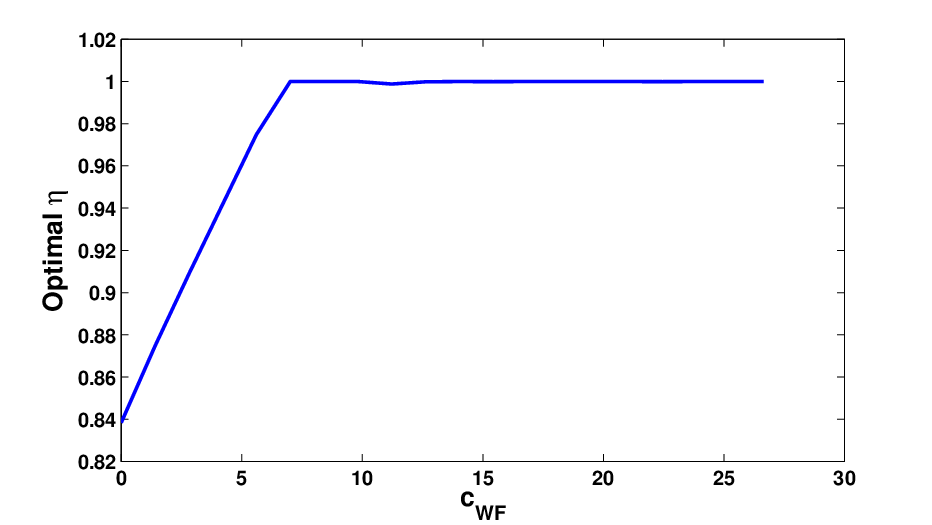
In Fig. 10, we show the adoption levels and for the sparse city at the WSP’s profit-maximizing operating point for a range of offloading benefits . Results for the small and dense cities are similar. We show the optimal coverage factors in Fig. 11; as we might expect from Fig. 8, the optimal value of increases with and eventually becomes 1.
We next vary the cost of deployment , keeping constant. Figure 12 shows the resulting adoption levels, with the optimal coverage factors shown in Fig. 13. For all cities, as the marginal cost of deployment increases, and the adoption of Technology 1 decrease. The decrease in is nonlinear: initially, as the cost of deployment is outweighed by the savings from offloading . The initial decrease from , however, is relatively rapid, as the decrease in due to decreasing is muted by an increase in adoption of the bundled technologies . For any fixed , the optimal coverage factor is largest for the dense city and smallest for the small city; this reflects the ordering of the marginal savings from offloading , which are largest for the dense city.
For the small city, the immediate decrease in the optimal coverage induces behavior similar to that of Fig. 7: as decreases (Fig. 13), adoption of the bundle first increases and then decreases as Technology 2 experiences greter congestion and less coverage. The same effect is observed for the sparse and dense cities, without the final decrease in for large (small ). Thus, in cities with denser populations, a decrease in coverage due to higher costs may in fact increase adoption of the bundled technologies.
VI Conclusion
In this paper, we develop a model of user adoption for base and supplemental wireless network technologies that accounts for heterogeneity in users’ technology valuations, congestion effects, and pricing decisions. We show that user adoption converges to a unique, stable equilibrium point, and derive analytical conditions under which non-intuitive adoption behaviors occur. We then show that these may persist when WSPs maximize either their revenue or profit. Our profit model incorporates both the savings from offloading and deployment costs of a WiFi network.

Though we use empirical data to realistically study WSP savings from offloading traffic onto a supplementary network, our parameters can only approximate true market structures. Similarly, our user adoption model makes approximating assumptions, one of which is that users’ technology valuations are uniformly distributed. We therefore show that many of the reported qualitative adoption behaviors are also observed for non-uniform distributions and nonlinear throughput functions (cf. Section IV-C and Appendix B). Our framework thus enables researchers to gain additional insights into the role of supplementary technologies in alleviating network congestion and the resulting economic implications.
Broadly speaking, our work fits into the framework of “Smart Data Pricing” (SDP), which studies new ways of pricing mobile data with the aim of making mobile data networks more operationally efficient [22]. While other SDP works have shown that users change their behavior in response to pricing policies such as time-dependent pricing [23], the framework introduced in this work can be used to investigate the effects of such pricing schemes on technology adoption levels when heterogeneous networks are present. Though such investigations are beyond the scope of this work, we anticipate that these smarter pricing policies can significantly improve WSP revenue and can even be used to steer the adoption levels to operationally favorable targets.
References
- [1] Electronista Staff, “Verizon preps LTE femtocells, says it hits limits in 2013,” Electronista, March 2012, http://www.electronista.com/articles/ 12/03/05/demand.for.mobile.data.will.outpace.build.out/.
- [2] S. Schroeder, “AT&T to add new Wi-Fi hotspots in New York and San Francisco,” Mashable, December 2010, http://mashable.com/ 2010/12/28/att-wi-fi-hotspots/.
- [3] Cisco Visual Networking Index, “Global mobile data traffic forecast update, 2011 - 2016,” May 2012, http://tinyurl.com/VNI2012.
- [4] S. Sen, C. Joe-Wong, S. Ha, and M. Chiang, “Incentivizing time-shifting of data: A survey of time-dependent pricing for Internet access,” IEEE Communications Magazine, vol. 50, no. 11, pp. 91–99, 2012.
- [5] Orange, “Orange pay monthly £2 wifi bundle terms and conditions,” 2013, http://e-gain.s3.amazonaws.com/external/content/Orange/ Terms%20and%20conditions/PAYM-2-pound-WiFi-bundle-terms.pdf.
- [6] S. E. Ante and R. Knutson, “Good luck leaving your wireless phone plan,” Wall Street Journal, July 2013, http://tinyurl.com/wsj-churn.
- [7] P. Geroski, “Models of technology diffusion,” Research Policy, vol. 29, no. 4-5, pp. 603–625, 2000.
- [8] V. Mahajan, E. Muller, and Y. Wind, New-Product Diffusion Models. Kluwer Academic, 2000, International Series in Quantitative Marketing.
- [9] M. Katz and C. Shapiro, “Technology adoption in the presence of network externalities,” The J. of Political Economy, pp. 822–841, 1986.
- [10] L. Cabral, “On the adoption of innovations with ’network’ externalities,” Mathematical Social Sciences, vol. 19, no. 3, pp. 299–308, 1990.
- [11] N. Economides and B. Viard, “Pricing of complementary goods and network effects,” EC-03-12, New York University, Tech. Rep., 2007.
- [12] D. Joseph, N. Shetty, J. Chuang, and I. Stoica, “Modeling the adoption of new network architectures,” in Proc. of ACM CoNEXT. ACM, 2007.
- [13] Y. Jin, S. Sen, R. Guérin, K. Hosanagar, and Z.-L. Zhang, “Dynamics of competition between incumbent and emerging network technologies,” in Proceedings of NetEcon. ACM, 2008, pp. 49–54.
- [14] S. Sen, Y. Jin, R. Guérin, and K. Hosanagar, “Modeling the dynamics of network technology adoption and the role of converters,” IEEE/ACM Trans. on Networking, vol. 18, no. 6, pp. 1793–1805, 2010.
- [15] S. Ren, J. Park, and M. van der Schaar, “Entry and spectrum sharing scheme selection in femtocell communications markets,” IEEE/ACM Trans. on Networking, 2012.
- [16] N. Shetty, S. Parekh, and J. Walrand, “Economics of femtocells,” in Proc. of IEEE GLOBECOM. IEEE, 2009, pp. 1–6.
- [17] S. Yaiparoj, F. Harmantzis, and V. Gunasekaran, “On the economics of GPRS networks with Wi-Fi integration,” European Journal of Operational Research, vol. 187, no. 3, pp. 1459–1475, 2008.
- [18] S. Yun, Y. Yi, D. Cho, and J. Mo, “The economic effects of sharing femtocells,” IEEE JSAC., vol. 30, no. 3, pp. 595–606, 2012.
- [19] P. Green and V. Srinivasan, “Conjoint analysis in consumer research: Issues and outlook,” Journal of Consumer Research, pp. 103–123, 1978.
- [20] R. Kim, “U.S. smartphone ownership eclipses feature phones,” GigaOm, May 2012, http://tinyurl.com/smart-feature-phones.
- [21] M. El-Sayed, A. Mukhopadhyay, C. Urrutia-Valdés, and Z. J. Zhao, “Mobile data explosion: Monetizing the opportunity through dynamic policies and QoS pipes,” Bell Labs Tech. J., vol. 16, no. 2, pp. 79–100, 2011.
- [22] S. Sen, C. Joe-Wong, S. Ha, and M. Chiang, “A survey of smart data pricing: Past proposals, current plans, and future trends,” ACM Computing Surveys, vol. 46, no. 2, 2014.
- [23] S. Ha, S. Sen, C. Joe-Wong, Y. Im, and M. Chiang, “TUBE: Time-dependent pricing for mobile data,” in Proceedings of ACM SIGCOMM. ACM, 2012, pp. 247–258.
- [24] H. K. Khalil, Nonlinear Systems, 3rd ed. Prentice Hall, 2002.
- [25] R. Schwartz and M. Johansson, “Carrier WiFi offload: Building a business case,” March 2012, Wireless 20/20 Business Case Tool.
Appendix A Proofs
A-A Proposition 1
A-B Proposition 2
In regions a, f and g, it is simple to show that the equilibria are stable: letting , we denote (11) as so that
at each equilibrium in regions a, f and g. Since this matrix is clearly negative definite, the equilibria are asymptotically stable.
In region b, the Jacobian of the dynamics (11) is
The eigenvalues of this matrix are , . Since we assume , both eigenvalues are real and negative and the equilibrium in region b is stable. Similarly, in region c the Jacobian has the form
which has eigenvalues satisfying
Upon simplifying, we find that , . As both of these are real and negative, we see that the equilibrium in region c is asymptotically stable.
Finally, in regions d and e we have the triangular Jacobian matrices
Since all diagonal entries in these matrices are negative, the equilibria in both regions are asymptotically stable. ∎
A-C Proposition 3
The result follows from Bendixson’s criterion. We can use the Jacobian expressions in the proof of Prop. 2 to show that the divergence of the dynamical equations (11) is negative in each region. Then Bendixson’s criterion tells us that no periodic orbits can exist.88 8 Bendixson’s criterion relies on Green’s theorem for the vector field , which is typically assumed to be continuously differentiable. In our case, is merely piecewise-linear and continuous. However, since we are working in and is continuously differentiable almost everywhere, the proof of Green’s theorem is still valid. Since no periodic orbits exist, each trajectory must converge to an equilibrium point. From Prop. 2, this equilibrium must be stable. ∎
A-D Theorem 1
The stability of the equilibrium follows from Prop. 2, while existence of at least one such equilibrium follows from the boundedness of the and the non-existence of a periodic orbit (Prop. 3). Thus, it remains to show that at most one equilibrium point can exist.
Suppose that two stable equilibrium points exist, and consider a bounded neighborhood of . We suppose that the dynamical equations (11) are continuously extended to all of for the purposes of the proof, and that no new equilibria are created. If we consider all trajectories lying in , the regions of attraction for both equilibria are (disjoint) open, connected, and invariant sets, whose boundaries are formed by trajectories [24]. However, since no periodic orbits exist, the boundaries must be the boundary of itself. Then since is connected, it cannot be a disjoint union of open sets, and there exists at least one point in that is in neither region of attraction. But this is a contradiction, as the trajectory starting from this point must approach a compact limit set. ∎
A-E Result 1
We first note from Table II that in regions a, b, f, and g of Table I, the total adoption remains constant at 1, i.e., full adoption. We may then differentiate the equilibrium expressions for and in region c and use the constraints in Table II to show that these quantities are increasing in . The remaining region is then region e, where (no users adopt the base technology), (some users adopt neither technology), and (some users adopt the bundled technologies). Differentiating Table II’s equilibrium expression for in this region, we find the condition (12). ∎
A-F Result 2
We first note from Table II that in regions a, b, e, f, and g in Table I, adoption of the base technology () does not depend on the price . In region d, we differentiate Table II’s expression for to find that it is decreasing in . Finally, we consider region c, where (some users adopt the base technology), (some users adopt the bundled technologies), and (some users adopt neither technology). We differentiate the equilibrium expression for to obtain the condition (13). ∎
A-G Proposition 4
By inspection, the optimal revenue in regions a, f, and g is non-positive in Table IV. Thus, since full adoption only occurs in regions a, b, f, or g and the bundled technologies have positive adoption in regions c and e, for the first part of the proposition it suffices to show that the revenue in regions b and d does not exceed that in regions c or e.
Region b: We first consider the case . By inspection, in this case region b has negative revenue. Since regions c, d and e have positive revenue, this cannot be optimal.
We now suppose that and . We show that the maximum revenue in region b is less than the maximum revenue in region e. It suffices, from Table IV, to show that
Simplifying and neglecting some terms, we find the sufficient condition
which is clearly true, since each term in the sum is nonnegative.
Next, we suppose that and show that the revenue at region c’s revenue-maximizing point is larger than the maximum revenue in region b. From Table IV, it suffices to show that
for any given , where
Multiplying out the fractions, we find the sufficient condition
We now expand the left side of this inequality; it is
We now obtain
Since the left-hand side is clearly negative, while the right-hand side is positive, we have the desired result.
Region d: We first show that the revenue in region c is increasing in . By inspection, the revenue expressions in regions c, d, and e are equal at and the optimal revenue in region d is independent of , which will complete the proof. We calculate that
where
Thus, for all values of . The revenue in region c for then exceeds that in region d. We note that since at , the expression in Table IV for region c’s maximum revenue is valid.
We next use the optimal revenue expressions in Table IV to show that for fixed , the revenue in region c exceeds that in region e if and only if
Since this expression is always nonnegative and region c’s revenue is increasing in , we see that the maximum revenue in region c occurs at , which exceeds that in region e. The maximum revenue thus occurs in region c, with . ∎
A-H Proposition 3
From the proof of Prop. 4, we see that for fixed , the maximum revenue occurs in region c if and only if
| (17) |
i.e., if (17) holds then at the revenue-maximizing prices, the equilibrium adoption levels lie in region c. If (17) does not hold, then the maximum revenue lies in either region d or region e. But we note that the revenue in regions d and e is the same at , and the revenue in region d does not depend on . In contrast, in region e the revenue increases with if (17) does not hold: we take the derivative of revenue in region e with respect to to find that it equals
where
Since , we see that this quantity is nonnegative, and thus that the revenue increases as increases. Revenue in region e thus exceeds that in region d for any value of not satisfying (17). No users adopt the base technology in region e (Table II), which completes the proof. ∎
A-I Result 4
The ISP’s revenue is maximized when the dynamics lie in region c if and only if . Thus, we can use Table IV’s expressions for the optimal prices in region c to find the corresponding adoption levels in Table II. Differentiating with respect to shows that total adoption increases with in region c, yielding the proposition. ∎
Appendix B Throughput Linearization
In Section III, we use linear models to represent the decrease in utility due to throughput degradation. We justify this assumption here by analyzing the accuracy of a linear approximation to previously proposed throughput measures.
Prior works on technology adoption [16] take congestion levels into account with a Markov chain analysis, assuming Poisson arrivals of rate and exponentially distributed session length with mean . The expected throughput is then
| (18) |
where is the average time of service without interference or queueing, and we assume . Thus, the throughput degradation equals (18), less the maximum throughput. We now use Taylor’s remainder theorem to bound the error of a linear approximation to (18). The second derivative of (18) is
where the infinite sum uses the Taylor series for and the geometric series for . Thus, approximating (18) at , we can bound the error by
Approximating the sum as the geometric series of , we let to obtain an upper bound of . Numerically, this bound is in fact conservative; for instance, taking and produces a maximum error of 0.013, as opposed to an analytical bound of 0.0625.


Having shown that linear functions can closely approximate proposed nonlinear throughput functions, we next investigate the dynamical behavior when the throughput degradation functions and are nonlinear. We take the throughput functions to be as in (18), i.e.,
| (19) |
where denotes the two technologies. Figure 14 shows the throughput functions (19) for and , 0.8; a different coefficient merely scales these functions and does not affect their qualitative shape. As expected from Appendix B, these functions are close to linear, though their slope clearly increases for larger (i.e., more congestion).
Figure 15 shows a range of simulations with (Figs. 15a and 15b) and (Fig. 15c) in (19). Figure 15a can be compared to Fig. 3a; in both figures, we observe a decrease in adoption of the bundled technologies and increase in adoption of the base technology for a large coverage factor . Total adoption increases for all values of in both cases. Figures 3b and 15b show a similar decrease in adoption of the bundled technology for large , but one in which adoption of the base technology is zero for larger values of . Finally, Fig. 15c shows that even when prices are chosen so as to maximize operator revenue, the adoption behavior with nonlinear throughput degradation functions mirrors that with linear throughput degradation, shown in Fig. 7. In both cases, we observe that the adoption of the base technology is initially zero, with adoption of the bundled technologies increasing with the coverage factor . After a threshold value of , however, adoption of the bundled technologies begins to decrease due to congestion on Technology 2, and adoption of Technology 1 correspondingly increases.
Appendix C Estimating Cost Parameters
Savings from Offloading: We take the marginal cost of 3G traffic during the peak hour to be 1.0 ¢/MB in the small city, 1.9 ¢/MB in the sparse city, and 2.9 ¢/MB in the dense city; these values are based on AT&T’s and Verizon’s data plan overage charges in the U.S. We next estimate , the probability that a 3G and WiFi user has access to WiFi in the hour of peak 3G usage, multiplied by this peak 3G usage. From our trial data, we find that each user consumes on average 1200MB in each month, with 660MB occurring at peak hours of the day. The probability of peak-hour WiFi access is 82% of the overall access probability; thus, the probability of WiFi access during the peak hour is . Each user then offloads ()(660MB) MB at the peak hours over one month (i.e., ). Multiplying by the ¢/MB marginal savings from offloading, we find that , 10.6, or 15.8 for the small, sparse, and dense cities respectively.
Deployment Costs: To find the marginal cost of deployment , we assume that each additional AP increases the coverage factor by a fixed amount and costs the WSP a fixed amount per month. From [25], we estimate as a monthly operational cost of $20, plus capital investment of $1200 spread over 12 months, so that = $120. For simplicity, we interpret the WiFi access probability as the physical area covered by APs, e.g., uniform user mobility. The cost of covering an area with APs is then . Normalizing by the user population, we find that
We use population densities of 2000, 5000, and 12000 people per square mile for the small, sparse, and dense cities respectively. The AP coverage area is assumed to be 0.01 square miles, (a 130 meter radius), for the small city, 0.005 square miles for the sparse city, and 0.002 square miles for the dense city. We then find , 4.9, and 11.5 for the small, sparse, and dense cities respectively.
Appendix D Extension to Multiple WSPs
We can extend our model to include multiple WSPs by adding additional adoption choices for users, e.g., adopting the base technology from another WSP. Conceptually, this change is simple: we simply formulate an additional utility function for each additional adoption choice, and then find the option that yields the highest utility for each value of . In practice, solving for the optimal choice for each user becomes complex due to the many possible orderings of the utility functions for different values of (i.e., extending Proposition 1 to multiple adoption choices). In this Appendix, we illustrate this complexity by considering two WSPs: one offering both the base and bundled technologies, and the other offering only the base technology. Each user then has four adoption choices: adopt no technology, adopt the base technology 1 from WSP 1, adopt the bundled technologies (1 + 2) from WSP 1, or adopt the base technology 3 from WSP 2.
We suppose that the utility of WSP 1’s base and bundled technologies is given by (1) and (2) as in Section III; the utility of WSP 2’s base technology is given analogously by
| (20) |
where as in Section III the intrinsic quality of the technology is captured in the variable , represents the negative externality experienced due to greater traffic on Technology 3, and is the access price. The fraction of users adopting Technology 3 is denoted by .
We next solve for the utility-maximizing adoption choice as a function of . As in Section III, we solve for the threshold values at which the ordering of different adoption choices changes. The thresholds , , and are as in Section III; the remaining thresholds are given by
where again denotes the threshold value of above which adoption choice yields higher utility than choice . To keep this meaning consistent, we suppose that ; if instead , the threshold should instead be denoted , and if , the threshold would become .
We next derive the analogue of Proposition 1 by enumerating the possible orderings of the thresholds:
Proposition 5
Suppose we are given the pairwise ordering of the following pairs of thresholds: (a) and ; (b) and ; (c) and ; (d) and ; (e) and ; (f) and ; and (g) and . Then for any user with , we can determine the adoption choice yielding the highest utility for this user.
Proof:
First, we show that the orderings (a–d) above imply the following:
- (a)
if and only if .
This is exactly the statement of Proposition 1.
- (b)
if and only if .
Suppose that . Then upon cross-multiplying the denominators and simplifying, is equivalent to
which is exactly the same expression obtained by simplifying the expression . Thus, the two inequalities are equivalent.
- (c)
if and only if .
Suppose that . We can cross-multiply and simplify to find the equivalent inequality
We can obtain the same inequality by simplifying . As in case (b), we thus obtain the proof in the other direction.
- (d)
if and only if .
As in cases (b) and (c) above, we first cross-multiply and simplify to obtain
Simplifying yields the same inequality, thus yielding the other direction of the proof.
We next show that for any two thresholds and where , the orderings (a–d) above allow us to determine whether or vice versa so long as the are not all distinct. We first note that at most two of can be equal, since and for all thresholds. We now divide the proof into three cases:
- •
Suppose that . Then without loss of generality, and . If or , then orderings (b) and (a) respectively determine whether or .
- •
Suppose that . Then or .
If , then and or . We must show that orderings (a-d) determine whether or , which is determined by orderings (b) and (a) if or respectively.
If , then and or . Orderings (c) and (d) respectively determine whether or if or respectively.
- •
Suppose that . Then or , and without loss of generality and . Then whether or is determined by orderings (c) and (d) respectively if or .
We can now conclude that given two thresholds and , their relative order is determined by inequalities (a–d) unless are distinct. In that case, since there are only four possible values for , and are ordered with respect to all other thresholds. Thus, we can order all six thresholds given inequalities (a–d) except in the case where no other threshold lies between and , in which case we must use orderings (e–g) to find the ordering of and . Since any user’s adoption choice is wholly determined by the orderings of the thresholds relative to the user’s value of , the proposition follows: the orderings (a–g) completely determine the ordering of the thresholds. ∎We next note that the seven orderings (a–g) cannot be chosen independently; for instance, if orderings (b) and (c) imply that , then ordering (a) must be . To enumerate all possible orderings, we introduce the “sign” of an ordering, which is if the ordering is the same as stated in Proposition 5, and if reversed. For instance, ordering (a) is if .
We first note that orderings (a) and (b) are independent. Ordering (c) is determined by orderings (a) and (b) if these orderings have opposite sign, so orderings (a–c) have 6 possible orderings total. From the proof of Prop. 5, ordering (d) is similarly determined by orderings (a–c) if any pair of these have opposite signs. Thus, orderings (a–d) yield 8 possible types of orderings for the six thresholds.
Orderings (e–g) can also not be chosen independently of orderings (a–d); these orderings serve as “tiebreakers” in the case that two thresholds with non-overlapping components end up placed consecutively. By explicitly enumerating the 8 possibilities of orderings (a–d), we find that two orderings require one tiebreaker each, and two others require two tiebreakers each. We thus find a total of 16 orderings of the six thresholds, which are as follows:
- 1.
- 2.
- 3.
- 4.
- 5.
- 6.
- 7.
- 8.
We use the notation to indicate that and are both valid pairwise orderings. Given these threshold orderings, one can then characterize different regions as in Table I and solve for each region’s adoption dynamics and equilibrium adoption point. It is then straightforward to solve for the equilibrium in each region and derive conditions under which each equilibrium point exists. One can then use such equilibria to examine, e.g., what proportion of users WSP 1 will gain from WSP 2 by introducing the supplementary technology.